the Creative Commons Attribution 4.0 License.
the Creative Commons Attribution 4.0 License.
 | 14 Oct 2021
Foreshock cavitons and spontaneous hot flow anomalies: a statistical study with a global hybrid-Vlasov simulation
Lucile Turc
Markus Battarbee
Jonas Suni
Xóchitl Blanco-Cano
Urs Ganse
Yann Pfau-Kempf
Markku Alho
Maxime Dubart
Maxime Grandin
Andreas Johlander
Konstantinos Papadakis
Minna Palmroth
The foreshock located upstream of Earth's bow shock hosts a wide variety of phenomena related to the reflection of solar wind particles from the bow shock and the subsequent formation of ultra-low-frequency (ULF) waves. In this work, we investigate foreshock cavitons, which are transient structures resulting from the non-linear evolution of ULF waves, and spontaneous hot flow anomalies (SHFAs), which are thought to evolve from cavitons as they accumulate suprathermal ions while being carried to the bow shock by the solar wind. Using the global hybrid-Vlasov simulation model Vlasiator, we have conducted a statistical study in which we track the motion of individual cavitons and SHFAs in order to examine their properties and evolution. In our simulation run where the interplanetary magnetic field (IMF) is directed at a sunward–southward angle of 45∘, continuous formation of cavitons is found up to ∼11 Earth radii (RE) from the bow shock (along the IMF direction), and caviton-to-SHFA evolution takes place within ∼2 RE from the shock. A third of the cavitons in our run evolve into SHFAs, and we find a comparable amount of SHFAs forming independently near the bow shock. We compare the properties of cavitons and SHFAs to prior spacecraft observations and simulations, finding good agreement. We also investigate the variation of the properties as a function of position in the foreshock, showing that transients close to the bow shock are associated with larger depletions in the plasma density and magnetic field magnitude, along with larger increases in the plasma temperature and the level of bulk flow deflection. Our measurements of the propagation velocities of cavitons and SHFAs agree with earlier studies, showing that the transients propagate sunward in the solar wind rest frame. We show that SHFAs have a greater solar wind rest frame propagation speed than cavitons, which is related to an increase in the magnetosonic speed near the bow shock.
- Article
(4616 KB) - Full-text XML
- BibTeX
- EndNote


As the supermagnetosonic solar wind interacts with Earth's magnetosphere, a curved bow shock forms upstream of Earth. The bow shock slows the solar wind down to submagnetosonic speeds while compressing and heating it. This allows the solar wind to flow around the magnetopause that separates the solar wind from the magnetosphere. At the quasi-parallel part of the bow shock (defined as the region where the shock normal and the interplanetary magnetic field (IMF) have an angle θBn<45∘), ions reflected off the shock can propagate several hundred ion inertial lengths upstream, forming the foreshock region. At the quasi-perpendicular shock (θBn>45∘), the upstream motion of the reflected ions is limited to approximately one ion gyroradius, and a more abrupt shock crossing is found.
The foreshock is characterised by instabilities arising due to the interaction between the backstreaming particles and the incoming solar wind. Depending on the angle θBn, a range of interesting features are found in Earth's foreshock. These include different shock-reflected suprathermal ion populations (e.g., Fuselier, 1995; Kempf et al., 2015), different types of ultra-low-frequency (ULF) waves (e.g., Hoppe et al., 1981; Greenstadt et al., 1995; Wilson, 2016) and a variety of transient structures (see Eastwood et al., 2005, for a review of the foreshock, and Zhang and Zong, 2020, for a recent review of foreshock transients).
Foreshock cavitons are transients that arise in Earth's foreshock due to the non-linear evolution of ULF waves. Cavitons are found amidst ULF waves and suprathermal ions, and they are identified as localised, highly correlated depressions in plasma density and magnetic field magnitude, bounded by rims where these parameters are enhanced. The extents of cavitons are of the order of 1 Earth radius (RE) with the plasma density and magnetic field magnitude decreasing by ∼50 % from their ambient solar wind values on average (Blanco-Cano et al., 2009, 2011; Kajdič et al., 2011, 2013). The temperature inside cavitons is similar to their surroundings, and they do not contain significant bulk flow deflections (Kajdič et al., 2013). While cavitons propagate sunward in the solar wind rest frame, they are carried back to the bow shock by the solar wind (Kajdič et al., 2011). Hybrid simulations (kinetic ions and fluid electrons) and spacecraft observations have demonstrated that the solar wind rest frame propagation speed often exceeds the Alfvén speed (Blanco-Cano et al., 2011; Wang et al., 2020).
Initially, the existence of cavitons was predicted using hybrid simulations (Lin, 2003; Lin and Wang, 2005). Also using hybrid simulations, Omidi (2007) and Blanco-Cano et al. (2009) proposed that under a radial IMF configuration, cavitons form when two types of ULF waves, parallel-propagating right- or left-hand polarised waves and obliquely propagating linearly polarised compressive waves, steepen and interact with each other. The presence of cavitons in spacecraft data was later confirmed with Cluster observations, where they were found to exist for a variety of different solar wind and IMF conditions (Kajdič et al., 2011; Blanco-Cano et al., 2011; Kajdič et al., 2013).
The term “caviton” was introduced by Blanco-Cano et al. (2009) to distinguish the transient type from foreshock cavities, which are similarly characterised by simultaneous density and magnetic depressions surrounded by rims of enhanced density and magnetic field magnitude (e.g., Sibeck et al., 2002; Schwartz et al., 2006; Billingham et al., 2011). Foreshock cavities form at isolated IMF flux tubes that are connected to the bow shock. As the field lines in these flux tubes are filled up with shock-reflected suprathermal particles, the plasma on the field lines expands, leading to a cavity where the plasma density and magnetic field magnitude are depressed (Schwartz et al., 2006). Unlike cavitons, foreshock cavities only contain suprathermal particles in their interiors but not in their surroundings due to their formation mechanism. Another difference is that cavitons are always surrounded by ULF waves, which is not necessarily true for foreshock cavities (e.g., Kajdič et al., 2017).
Another class of transients found in Earth's foreshock are hot flow anomalies (HFAs) (e.g., Schwartz et al., 1985; Schwartz, 1995; Lucek et al., 2004) which form when a tangential discontinuity in the IMF interacts with the bow shock and confines suprathermal ions in its vicinity. HFAs are also characterised by simultaneous depressions in plasma density and magnetic field magnitude bounded by enhancements, but they further display a significantly elevated temperature and a highly deviated bulk flow inside them. Signatures of HFAs in the absence of IMF discontinuities led to the identification of a separate transient phenomenon, spontaneous hot flow anomalies (SHFAs) (Zhang et al., 2013; Omidi et al., 2013). SHFAs are thought to evolve from cavitons when they are advected to the bow shock by the solar wind and they accumulate suprathermal ions. Global hybrid simulations have shown that the arrival of multiple SHFAs at the bow shock can cause the bow shock surface to erode (Blanco-Cano et al., 2018) and that SHFAs can impact the magnetosheath between the bow shock and the magnetopause by causing the formation of magnetosheath filamentary structures (Omidi et al., 2014a) or magnetosheath cavities and magnetosheath jets (Omidi et al., 2016). Omidi et al. (2016) also reported that the pressure variations caused by SHFAs and magnetosheath cavities can lead to the motion of the magnetopause.
Cavitons and SHFAs have been studied statistically in the past by using observations from the Cluster spacecraft. Kajdič et al. (2013) studied a set of 92 cavitons observed between 2001–2006, and Kajdič et al. (2017) later extended the statistical study to include other transients as well, including 19 observations of SHFAs from 2003–2011. Both cavitons and SHFAs were found for various solar wind conditions, and they were observed within 9 and 6 RE from the bow shock, respectively (as measured along the IMF direction). Kajdič et al. (2013) observed cavitons preferentially during stronger IMF, lower solar wind density, and larger solar wind and Alfvén speeds. Based on the speed of the solar wind and the duration of the cavitons in spacecraft data, Kajdič et al. (2013) estimated the extents of the cavitons to be in the range of 1–13 RE. Inside cavitons, the plasma density and magnetic field magnitude decreased by 20 %–90 % from their solar wind values, with an average decrease of 50 %. The observed SHFAs were very depleted, showing average decreases of 90 % in the density and magnetic field magnitude from their solar wind values. However, the magnitude of the depletions inside SHFAs listed by Kajdič et al. (2017) may be a product of the strict criteria used by the authors for detecting the events. Other spacecraft observations of potential SHFAs by Wang et al. (2013) and Chu et al. (2017) show numerous transients with <90 % decreases in the density and magnetic field magnitude.
Using global hybrid simulations, Omidi et al. (2014b) studied the variation of SHFAs' properties with parameters such as Alfvén Mach number (MA), IMF cone angle and the transients' distance from the Sun–Earth line. A low SHFA formation rate was found for MA≤3, with the rate increasing with MA. The formation rate showed no clear dependence on the IMF cone angle, and a run with a cone angle of 90∘ demonstrated that SHFAs can form even under such geometry. Omidi et al. (2014b) found that increasing MA resulted in the SHFAs having stronger features, such as larger magnetic enhancements at the transients' edges along with greater ion temperatures and greater levels of solar wind deceleration. Further, the duration of the SHFAs did not show dependence on the Mach number, which suggests that their size also increases with MA. Formation of SHFAs occurred preferentially close to the bow shock nose, where the transients exhibited larger temperatures compared to the ones located further away from the nose. Close to the bow shock nose, SHFAs also tended to have stronger magnetic enhancements and greater levels of solar wind deceleration, but these features were found to be less noticeable at lower MA.
The statistical studies of Kajdič et al. (2013, 2017) and Omidi et al. (2014b) have helped in establishing a global picture of cavitons and SHFAs in Earth's foreshock, but there are still many details in this picture that are not well understood. In particular, open questions concerning the evolution of the transients include the following. Where and how often do cavitons emerge in the foreshock? How do their properties evolve as they are advected towards the bow shock by the solar wind? Do all cavitons evolve into SHFAs? In the present paper, we aim to understand the evolution of cavitons and SHFAs in Earth's foreshock by performing a statistical study of these transients with the global hybrid-Vlasov simulation model Vlasiator (von Alfthan et al., 2014; Palmroth et al., 2018). By tracking the motion of individual cavitons and SHFAs in a simulation run with an IMF vector directed at a 45∘ sunward–southward angle, we have studied the properties and the evolution of 1445 transients, the largest statistical sample up to date. We first examine and compare the physical properties of cavitons and SHFAs, such as their density and magnetic field depressions, ion temperature, bulk flow speed and size. We then present statistical maps of the formation locations of cavitons and SHFAs, and we study the rate of caviton-to-SHFA evolution throughout the foreshock. We also investigate the variation of the properties of the transients as a function of the distance from the bow shock and the Sun–Earth line. Finally, we calculate the propagation velocities of the transients, presenting the first large sample statistical results of the propagation of cavitons and SHFAs.
2.1 Vlasiator simulation
We study foreshock cavitons and SHFAs using the Vlasiator model (von Alfthan et al., 2014; Palmroth et al., 2018), which is a hybrid-Vlasov code designed for performing global simulations of Earth's magnetosphere and the space surrounding it, capable of resolving ion kinetic effects. In the hybrid-Vlasov approach, ions are modelled using velocity distribution functions (VDFs), which evolve according to Vlasov's equation, and electrons are modelled as a cold, massless charge-neutralising fluid. In Vlasiator, Vlasov's equation is coupled to Maxwell's equations, and the system is closed with Ohm's law including the Hall term. Ion VDFs are discretised on a 3D Cartesian grid where a sparse grid representation is utilised in order to maintain numerical efficiency.
The simulation run used in our study is the same that has been previously used by Blanco-Cano et al. (2018) to study cavitons and SHFAs, and by Hoilijoki et al. (2019) to study dayside magnetic reconnection and flux transfer events (FTEs). The run is 2D in ordinary space and 3D in velocity space. The simulation is performed in the noon–midnight meridional plane and it uses the Geocentric Solar Ecliptic (GSE) coordinate system. In this system, Earth is located at the origin, the x axis is directed towards the Sun, the z axis is perpendicular to the ecliptic plane and the dusk-directed y axis completes the coordinate system. Our simulation domain covers [−48.66, 64.35 RE] in the x direction, [−59.65, 39.24 RE] in the z direction and a single cell in the y direction. The simulation has a spatial resolution of 300 km and a velocity space resolution of 30 km s−1. The solar wind enters the simulation domain from the positive X boundary, and other boundaries of the domain use copy conditions. In the out-of-plane y direction, periodic boundary conditions are used. The inner boundary of the simulation corresponds to a perfectly conducting ionosphere represented by a static Maxwellian distribution, located at 30 000 km (∼4.7 RE) from the origin. Earth's geomagnetic field is modelled as a 2D line dipole (Daldorff et al., 2014) with the tilt neglected.
In our run, the solar wind has a velocity of km s−1. Protons are the only ion species present, with a number density nSW=1.0 cm−3 and temperature TSW=0.5 MK in the solar wind, corresponding to fast solar wind conditions. The IMF is set to nT, directed sunward and southward with a cone angle of 45∘ and a total magnitude of 5 nT. With these parameters, the solar wind in our simulation run has β=0.7, magnetosonic Mach number Mms=5.6 and Alfvén Mach number MA=6.9. The proton inertial length and the proton gyroradius ri in the solar wind are km and ri=214 km, respectively. The duration of the simulation is 1437.5 s, with the state available at 0.5 s intervals.
2.2 Detecting and tracking foreshock transients
To detect cavitons and SHFAs, we define them as structures where both the proton number density n and the magnetic field magnitude B are below 80 % of their respective ambient solar wind values. These criteria have been previously utilised by Blanco-Cano et al. (2018) in their Vlasiator study and by Kajdič et al. (2013, 2017) in Cluster observations. The caviton events selected by Kajdič et al. (2013, 2017) additionally had to fulfil another criterion, which we have omitted from the present study. This criterion is based on a function χ(t), defined as , with 〈〉 denoting average values over the studied time interval. For an event to be recognised as a caviton, the value of χ(t) during the event had to exceed 〈χ〉 calculated for the studied time interval by at least 5 standard deviations. In the present study, we do not utilise this criterion in order to be able to detect small transients and capture the transients' full evolution from ULF waves into fully developed transients. In our simulation run, the thresholds for n and B are 0.8 cm−3 and 4.0 nT, respectively. In order to distinguish SHFAs from cavitons, we require that SHFAs fulfil an additional criterion of having β>10 in at least 60 % of the cells belonging to a transient. This criterion was previously used by Blanco-Cano et al. (2018), and it is chosen in order to not make assumptions on the level of heating and flow deflection inside the transients. A value of 10 indicates that the transients are dominated by the plasma instead of the magnetic field, and it is significantly above the typical β in the surrounding foreshock (β∼1–4).
To study cavitons and SHFAs evolving in time, we identify individual transients and track their motion over their lifetime. We begin the tracking procedure at t=900.0 s, when the bow shock and the foreshock appear well formed, and continue the tracking until t=1437.5 s, resulting in a total time interval of 537.5 s. We first identify all simulation cells fulfilling the caviton criteria at each time step of the tracking time interval. We exclude the cells located earthward of the bow shock by introducing a boundary based on a fourth-order polynomial fit of the shock. The boundary is updated at each time step in order to account for the outward motion of the bow shock due to 2D effects, and it is shifted earthward by 3.5 RE from the calculated position of the fit to account for irregularities in the bow shock. After we have found all the cells that fulfil the caviton criteria, we sort the cells into individual transients.
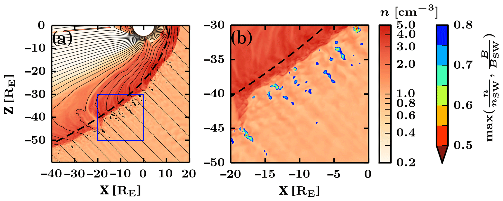
Figure 1Two zoomed-in views of the studied Vlasiator simulation run showing the foreshock at t=1012.5 s. The background colour displays the proton number density n (left colour bar), and the thin black continuous lines represent the magnetic field B. Panel (a) shows cavitons and SHFAs marked in black. The area delimited by the blue square is shown in panel (b), where the transient depth (defined as the maximum between n and the magnetic field magnitude B normalised by their solar wind values) is shown (right colour bar). The thick dashed line represents the boundary behind which cells fulfilling the caviton criteria are ignored.
Figure 1 shows two zoomed-in views of the simulation run used in this study at t=1012.5 s. A global view of the foreshock is shown in Fig. 1a, where cavitons and SHFAs are highlighted in black (no distinction between the transient types). A dashed line shows the boundary delimiting the area earthward of the bow shock. Cavitons and SHFAs are found deep in the foreshock, as is suggested by the fluctuations seen in the background colour map displaying the proton number density. Several transients exhibit elongated shapes and are found together in “chains” that are aligned with the direction of the IMF. These chains are a recurring feature in our simulation, and they are found amid ULF waves that propagate at different angles, offering suitable conditions for continuous transient formation. Figure 1b shows a further zoomed-in view that illustrates the interior structure of cavitons and SHFAs. The colour scale inside the transients represents the “depth” of the transients, which we define as the maximum value between the proton number density and the magnetic field magnitude normalised by their solar wind values. Many of the transients have complex interiors, where either one or multiple density/magnetic field minima can be observed. We find that such complex structures arise as multiple transients interact with each other and merge. Conversely, large transients occasionally split up and form multiple smaller transients.
We track the motion of cavitons and SHFAs by identifying overlapping transients at consecutive time steps. The overlapping transients are either advecting, splitting into multiple transients or merging together. Using this method, we reconstruct the history of each tracked transient. We set a lower limit for transient overlap at 25 % of the smaller transient's cell count, and we require the tracked transients to have a size of at least 5 cells (∼0.011 ). This is done in order to ensure consistent tracking of the smallest transients. Additionally, we monitor disappeared transients for overlapping for 5 s (10 time steps) to improve the tracking of shallow transients. After the tracking, we categorise the transients using the SHFA criterion. We use three general categories, which are “pure cavitons” that never fulfil the SHFA criterion during their lifetime, “pure SHFAs” that always fulfil the SHFA criterion during their lifetime and “evolving transients” that fulfil the SHFA criterion only part of their lifetime.
During our tracking time interval spanning 537.5 s, we have tracked a total of 1445 unique transients. We detected 1272 (88.0 %) independently forming transients and 133 (9.2 %) transients that split off from existing transients. In total, we detected 274 merging events between the tracked transients. At the beginning of our tracking interval, we detected 40 (2.8 %) transients, which we have omitted from our formation and propagation statistics as it is unclear whether these transients existed prior to the tracking interval. At any given time, we observe 29–72 simultaneous transients in the foreshock, and we find the average number of simultaneous transients to be 51. At all times, the number of observed cavitons exceeds the number of observed SHFAs. The percentage of cavitons varies between 56.8 %–88.6 %, with an average percentage of 74.8 %. In terms of transient evolution, we find that pure cavitons make up half of the tracked transients (725, 50.2 %), while pure SHFAs (342, 23.7 %) and evolving transients (378, 26.1 %) represent roughly a quarter each. The majority of the evolving transients are cavitons that evolve into SHFAs (341, 23.6 %), while the rest (37, 2.5 %) are either transients that change their classification momentarily or SHFAs that evolve into cavitons. The individual examples of “SHFA-to-caviton evolution” are due to our classification method and we do not find evidence of such evolution being recurrent.
Table 1Statistics of the physical properties of the tracked transients. The columns show the 25th/50th/75th percentile values, the mean value and the sample size (N) for each property listed in the left column. The presented properties are extrema over transient lifetime. The transients are classified into cavitons and SHFAs according to their type at each property extremum. From top to bottom: Total proton number density n, solar wind core proton number density nc, suprathermal proton number density nst, magnetic field magnitude B, proton temperature T, plasma β, bulk flow speed vflow and transient area A. The densities and the magnetic field magnitude are normalised to the input solar wind values.
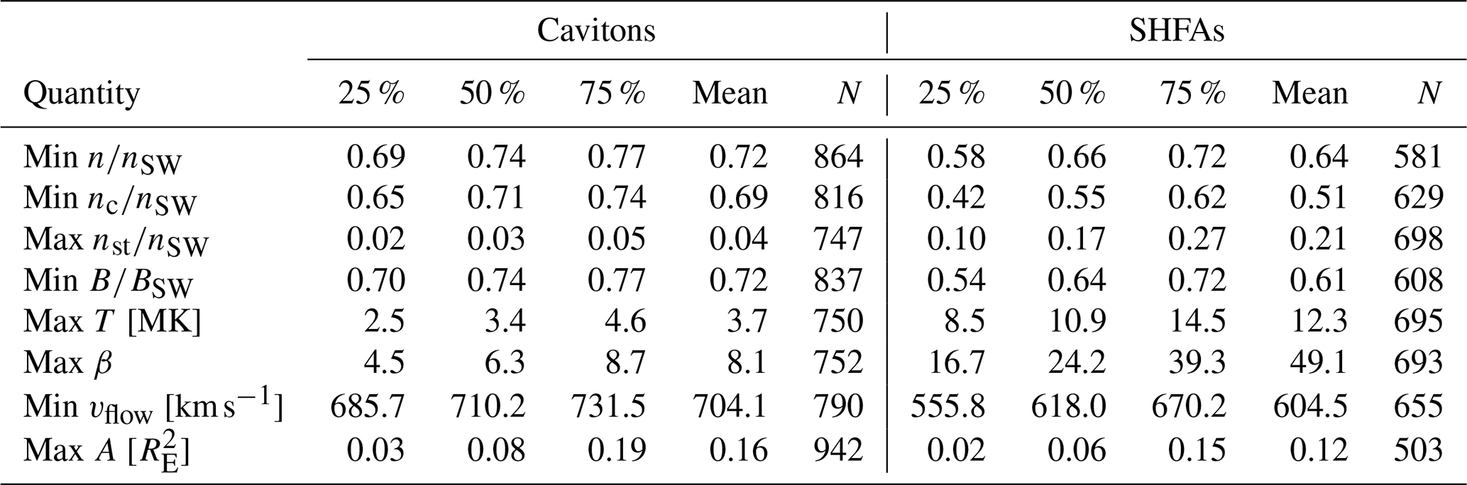
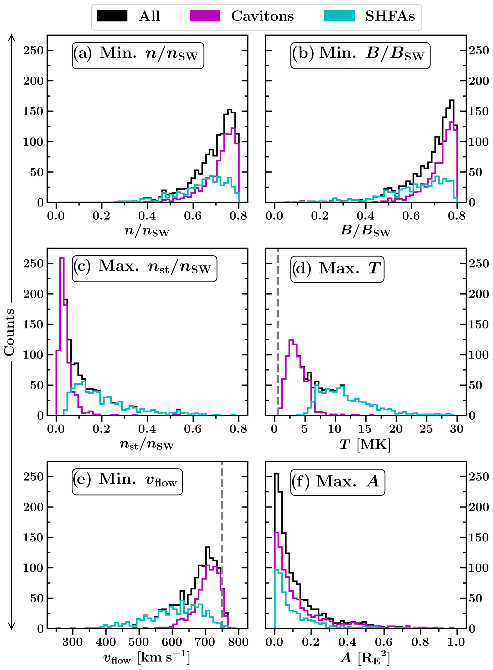
Figure 2Histograms visualising the distributions of selected quantities from Table 1. The grey dashed lines in panels (d) and (e) represent ambient solar wind values. Panels (d) and (f) contain outliers beyond 30 MK and 1 which have been excluded for clarity.
3.1 Physical properties
In Table 1, we present statistics of the physical properties of the tracked cavitons and SHFAs. We have looked at the extrema of the properties occurring during the transients' lifetime, such as the minimum density, magnetic field magnitude and bulk flow speed and the maximum temperature and area. For each property, we have categorised the transients into cavitons and SHFAs based on their type at the time when the extremum of the property was reached. In Fig. 2, we visualise some of the distributions of the properties presented in Table 1. In order to compare the properties of the tracked transients with those of the surrounding foreshock, we have measured the same properties at the troughs of general foreshock density fluctuations (not shown in Table 1). We define these troughs as the local minima of the proton number density below the input solar wind proton number density. For the comparison, we pick only troughs in a relevant region, i.e., in the region where either cavitons are present (10 RE from the bow shock, as measured along the IMF direction) or SHFAs are present (4 RE from the shock, see Sect. 3.2 for more details).
Inside cavitons (SHFAs), the total proton number density n and magnetic field magnitude B decrease from their input solar wind values up to 61 % (73 %) and 88 % (94 %), respectively. For n, a mean decrease of 28 % is found for cavitons, and a mean decrease of 36 % is found for SHFAs. For B, the mean decreases are 28 % for cavitons and 39 % for SHFAs. The mean decrease in n for all density troughs in the foreshock within 10 RE from the bow shock is 12 %. The mean deviation of B in these troughs has a similar value (10.9 %). Moreover, fluctuations with density decreases exceeding our transient detection limit of 20 % represent 17.4 % of all fluctuations in this range. These values show that the transients selected by our criteria are deeper than the typical fluctuations in the surrounding foreshock. Figure 2a and b show that the decreases inside cavitons are mostly concentrated near the transient detection limit while the decreases inside SHFAs are distributed more evenly across their respective value ranges. We see that the number of SHFA data points exceeds the number of caviton data points when n and B decrease below ∼65 % of their solar wind values, indicating that SHFAs tend to be more depleted than cavitons.
Next, we compare the number density of suprathermal protons inside cavitons and SHFAs. We consider the suprathermal population to consist of all protons outside the solar wind core population, which is centred around the solar wind bulk velocity within a 500 km s−1 sphere in the velocity space. The separation of the core and suprathermal populations is done automatically as the simulation is run, and its results are valid as long as the solar wind core population is not too strongly decelerated or heated in the foreshock. We note that while initially separate core and suprathermal populations may produce a single-component velocity distribution inside highly developed foreshock transients (e.g., Thomsen et al., 1988; Archer et al., 2015; Schwartz et al., 2018), the flow deflections inside the SHFAs in our run are mostly due to the impact of a separate suprathermal population. Therefore, our estimate of the suprathermal density is reliable inside the transients.
The suprathermal number density (nst) is clearly larger inside SHFAs than inside cavitons. A mean value of 0.21nSW is found inside SHFAs (nSW being the solar wind proton number density), while the mean value for cavitons is 0.04nSW. Figure 2 shows that nst rarely exceeds 0.15nSW inside cavitons but routinely reaches high values inside SHFAs, with an overall maximum density of 0.78nSW. To verify that the high values inside SHFAs are not due to individual cells but represent an overall increase in the amount of suprathermals, we repeated the analysis using the maximum average value of nst instead of the overall maximum value, and we found the results to be similar. The mean suprathermal number density in a trough of a foreshock fluctuation within 10 RE from the bow shock is similar to the mean value for cavitons (0.03nSW). The mean value in the region where SHFAs are found (<4 RE) remains similar (0.05nSW) and is small compared to the values found inside SHFAs. This shows that the suprathermal number density inside cavitons remains similar to their surroundings. While the amount of suprathermals is enhanced inside SHFAs, the mean solar wind core number density (nc) inside SHFAs (0.51nSW) is lower than that inside cavitons (0.69nSW) and the surrounding ULF fluctuations (0.79nSW within 4 RE from the shock).
In accordance with the elevated amount of suprathermals, higher proton temperatures (T) and lower bulk flow speeds (vflow) are found inside SHFAs compared to cavitons and the surrounding foreshock. Notably, Fig. 2d shows a clear cut-off temperature between cavitons and SHFAs at ∼7 MK (14 times the solar wind proton temperature TSW). The sharp cut-off is likely due to our β-based SHFA criterion. Nevertheless, the distribution of T shows cavitons distributed around a value of ∼3 MK (mean 3.7 MK), while SHFAs form a tail extending to ≳20 MK (mean 12.3 MK). The overall highest temperature inside an SHFA is ∼50.0 MK, which occurred due to individual transient cells interacting with the bow shock. The mean temperature inside troughs of foreshock density fluctuations within 4 and 10 RE from the bow shock are 4.3 and 2.8 MK, respectively. These values are similar to those found inside cavitons, verifying that cavitons have similar temperature as in their surroundings, while the temperature inside SHFAs is notably higher.
Figure 2e shows that no similar cut-off is seen between cavitons and SHFAs for the bulk flow speed as for the temperature. The bulk flow speed inside cavitons is generally above ∼600 km s−1 (∼20 % decrease from the solar wind bulk flow speed), and a mean value of 704.1 km s−1 (6.1 % decrease) is found. Compared to cavitons, SHFAs exhibit a larger range of bulk flow speeds extending to ≲400 km s−1 (≳46.7 % decrease) and have a lower mean bulk flow speed (604.5 km s−1) (19.4 % decrease). The mean bulk flow speed for troughs of foreshock fluctuations within 10 RE from the bow shock is 728.2 km s−1 (2.9 % decrease). This value corresponds to the peak of the caviton bulk flow speed distribution, but slower bulk flow speeds are also found inside cavitons, which should only exhibit minor bulk flow deflections. We note that several cavitons with low bulk flow speeds evolve into SHFAs later in their life but have their bulk speed minima occur while the transients are still classified as cavitons. The cavitons and SHFAs with moderate bulk flow speed reductions (∼10 %–20 %) might be better described as “proto-SHFAs”, which do not contain significant bulk flow deflections and are yet to develop into mature SHFAs (Zhang et al., 2013).
Cavitons and SHFAs do not inherently differ in terms of transient size. Figure 2f shows that the maximum areas of both types have similar distributions. Most transients are small, with ∼78 % of all tracked transients having a maximum area of <0.2 . The overall largest transient (1.91 ) is a result of mergers between smaller transients, and the largest transient not involved in mergers has an area of 1.02 . Cavitons have a slightly larger mean maximum area (0.16 ) compared to SHFAs (0.12 ), which likely results from SHFAs forming only close to the bow shock, where they do not have time to grow large. Accordingly, we find that the evolutionary track of the transients influences the transient sizes. Pure SHFAs have the smallest mean area (0.08 ), followed by pure cavitons (0.11 ) and evolving transients (0.27 ), which represent the longest-lived structures.
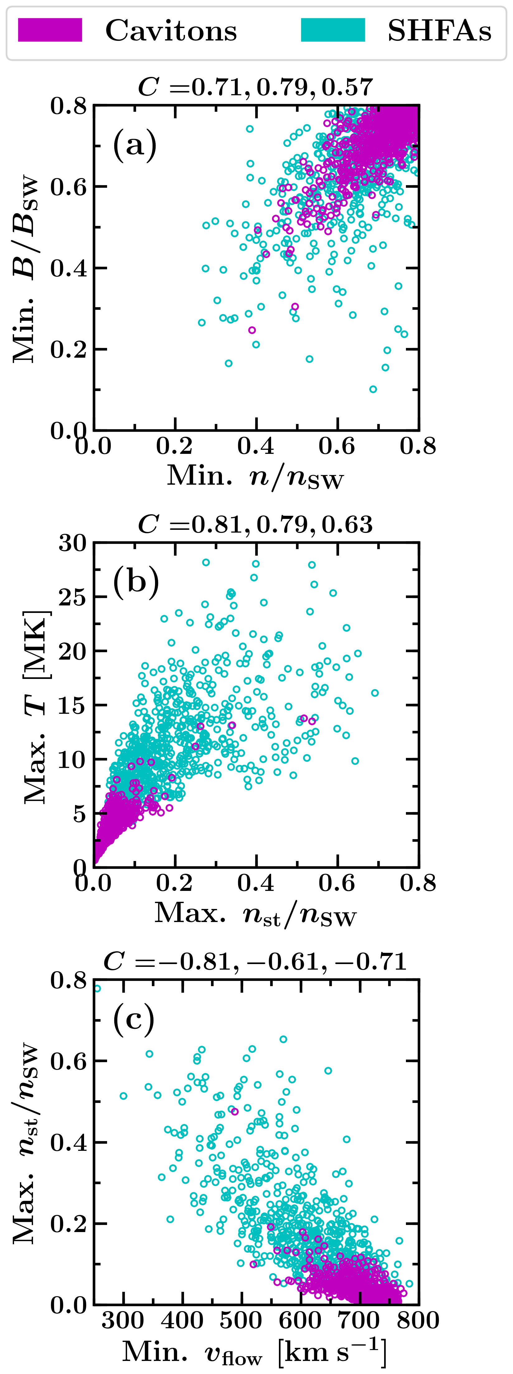
Figure 3Scatterplots showing the correlations between different quantities for the tracked transients. The Pearson correlation coefficients (labelled C) are shown above each panel for all transients, cavitons (magenta) and SHFAs (cyan), respectively. The values on the x axis are overall extreme values over tracked transients' lifetimes and the values on the y axis are extreme values taken from the same time step as the values on the x axis.
We looked for possible correlations between the physical properties presented in Table 1. In Fig. 3, we present a set of three scatterplots illustrating the correlation between selected properties that represent the characteristics of cavitons and SHFAs. The values are chosen such that the values on the x axis represent extrema over transient lifetime and the values on the y axis are extrema taken from the same time step as the values on the x axis. We have calculated the Pearson correlation coefficient in each scatterplot for all transients, cavitons and SHFAs separately.
Figure 3a shows the correlation between the minima of the proton number density n and the magnetic field magnitude B normalised by their solar wind values nSW, BSW. When both cavitons and SHFAs are considered together, a correlation coefficient of C=0.71 is obtained. Separately, cavitons show a good correlation (C=0.79), while the correlation for SHFAs is weaker (C=0.57). In general, the distribution shown in Fig. 3a represents an extension of the overall foreshock ULF wave field. This indicates that there is no clear limit between the transients and the surrounding ULF wave field as the transients form due to the non-linear interaction of foreshock ULF waves. Figure 3b shows the correlation between the maxima of the suprathermal proton number density nst and the proton temperature T. For cavitons and SHFAs combined, a good correlation is found (C=0.81). For low nst (≲0.25nSW), T increases in concert with nst, which is reflected by the correlation coefficient for cavitons (C=0.79). For larger nst (≳0.25nSW), the correspondence between nst and T becomes less linear, which is also apparent in the correlation coefficient for SHFAs (C=0.63). It is noteworthy that there is no clear cut-off between cavitons and SHFAs in terms of nst, and a wide range of T exists in the “transition region” between cavitons and SHFAs (∼0.05–0.20nst). In Fig. 3c, a good correlation is also found between the minimum bulk flow speed vflow and maximum nst for cavitons and SHFAs combined (), with vflow decreasing with increasing nst. Similar to T, a wide range of vflow is seen for each nst. However, unlike T, vflow appears better correlated for large nst (SHFAs, ) than for small nst (cavitons, ).
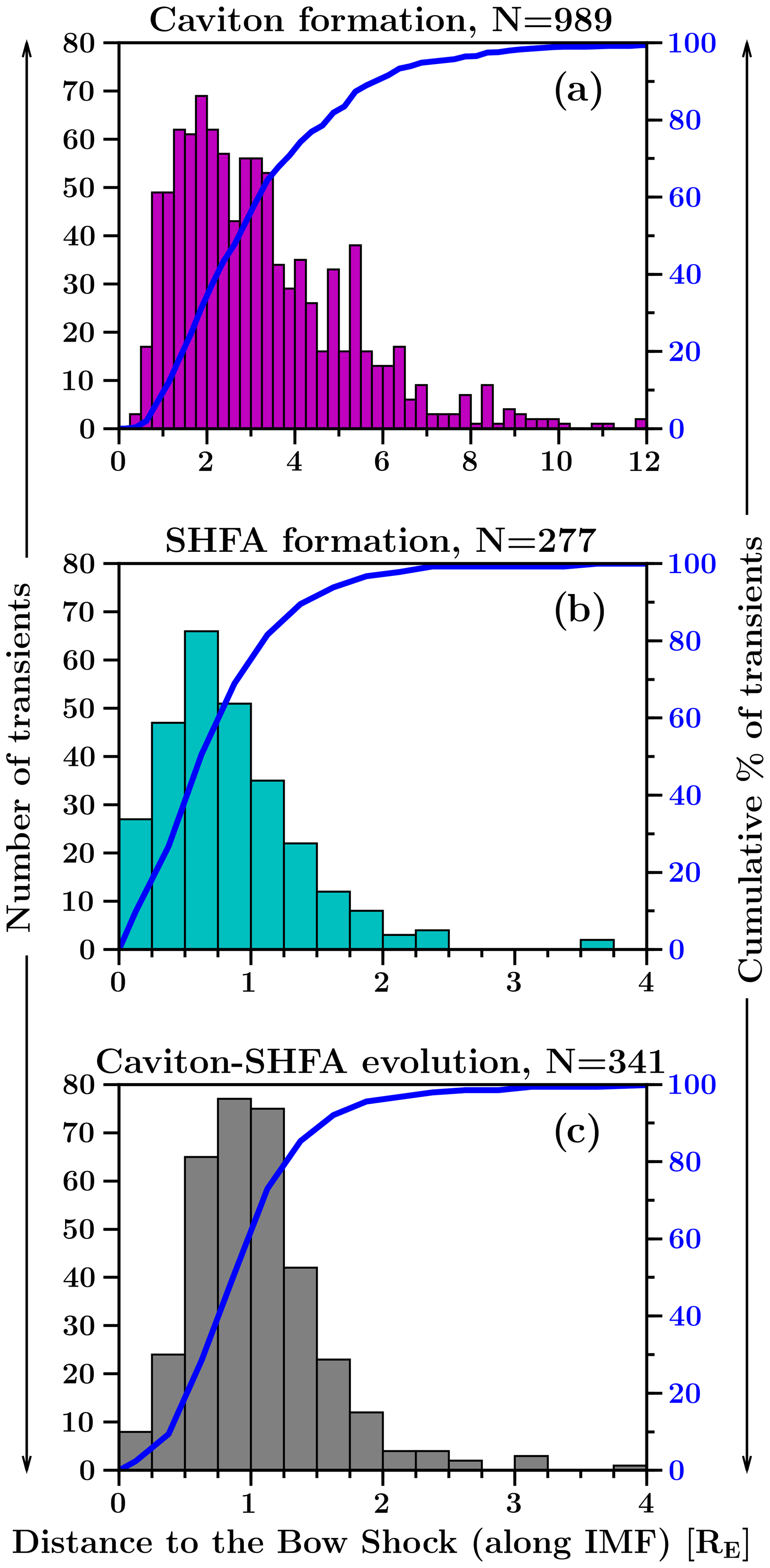
Figure 4Distributions of (a) the caviton formation locations, (b) the SHFA formation locations and (c) the locations where caviton-to-SHFA evolution takes place as a function of the distance to the bow shock along the IMF direction (45∘ angle from the Sun–Earth line). The blue curve in each panel shows the cumulative distribution.
3.2 Transient formation and evolution
Throughout our tracking interval, we find a steady rate of transient formation with no extended periods of increased/decreased formation. By taking a 10 s moving average, we find that the transient formation rate fluctuates between ∼1–4 transients forming per second, with an average of ∼2.4. In Fig. 4, we present the distributions of caviton formation locations, SHFA formation locations and the locations where caviton-to-SHFA evolution takes place as a function of the distance from the bow shock measured along the IMF direction. For this measurement, we consider the bow shock to be located at the first cell in which the solar wind core temperature is at least 4 times the ambient solar wind temperature (see Wilson et al., 2014, and Battarbee et al., 2020, for the application of this method on spacecraft and simulation data, respectively). Since some transients change their classification between a caviton and an SHFA multiple times, we consider only the final change from a caviton into an SHFA counting as a caviton turning into an SHFA.
Figure 4a shows that continuous formation of cavitons extends up to ∼10 RE from the bow shock, accounting for ∼99 % of all caviton formation (6 outliers forming at 12.6–39.5 RE are excluded from the figure). The median of the formation locations is at 2.8 RE, and the formation of cavitons is most abundant within ∼4 RE from the bow shock, where ∼70 % of all cavitons form. There is no caviton formation very close to the shock, with the nearest caviton forming at a distance of 0.3 RE. Figure 4b and c show that SHFAs either form independently without a prior caviton stage (Fig. 4b) or evolve from cavitons (Fig. 4c) within ∼4 RE from the bow shock (note the different extent but equal bin width on the x axis compared to Fig. 4a). The median of the formation (evolution) locations is found at 0.7 RE (1.0 RE). There is a slightly higher number of SHFAs evolving from cavitons (N=341) compared to independently forming SHFAs (N=277). The rates of independent SHFA formation and caviton-to-SHFA evolution are very similar. Most SHFAs emerge within ∼2 RE from the bow shock, which accounts for ∼96 % of SHFA formation and ∼95 % of caviton-to-SHFA evolution. A minor difference between SHFA formation and evolution is that the formation rate peaks slightly closer to the shock (∼0.5–0.75 RE) than the evolution rate (∼0.75–1.0 RE), and the formation rate is generally higher near the shock (≲0.5 RE). Approaching the bow shock, the number of SHFAs relative to cavitons increases, and the SHFA formation rate surpasses the caviton formation rate at ∼0.8 RE. Still, a notable amount of cavitons is found near the bow shock and not all cavitons evolve into SHFAs. Within 1.5 RE from the shock, a total of 180 cavitons form, of which ∼59 % evolve into SHFAs.
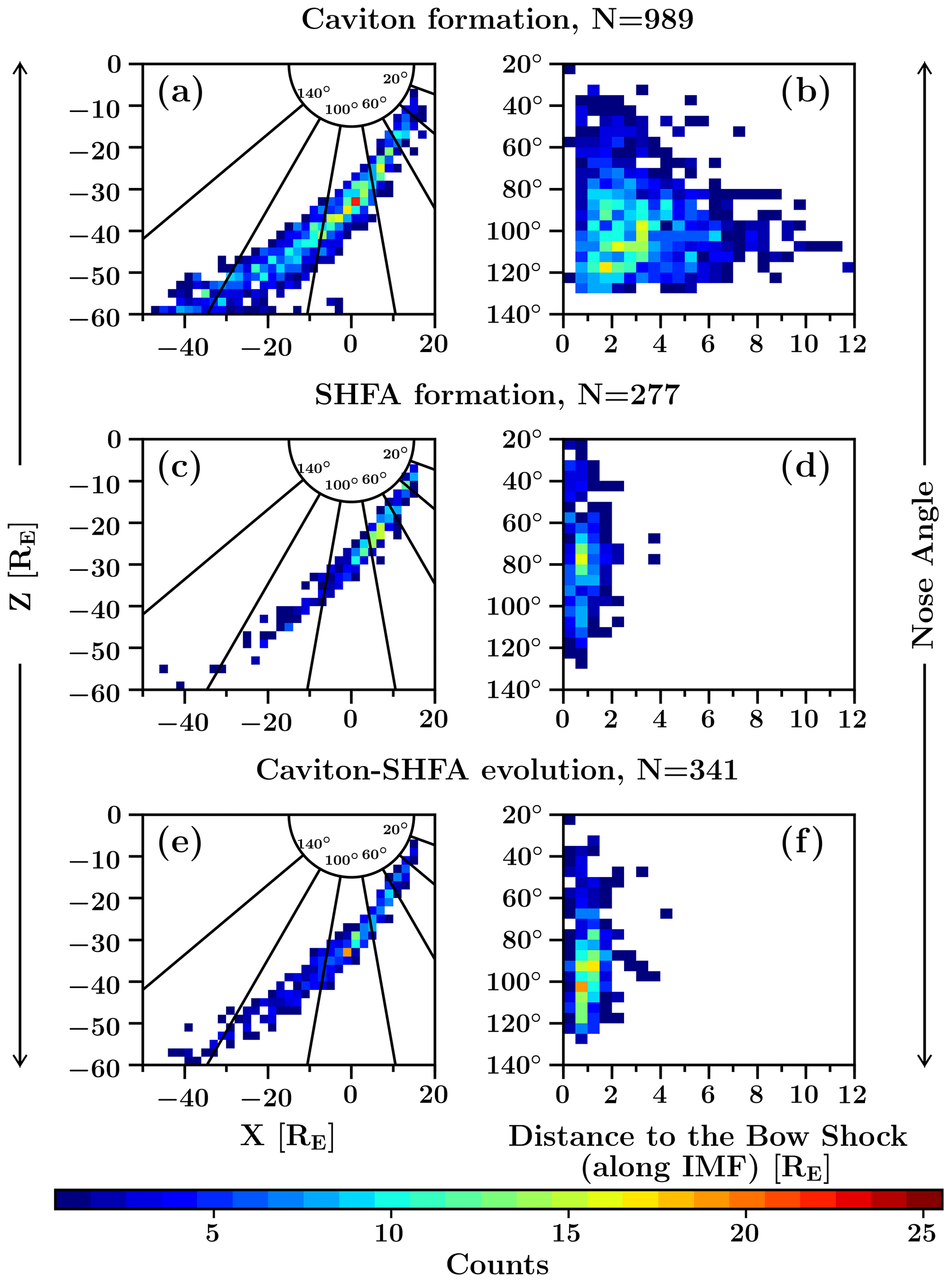
Figure 52D distributions of the caviton formation locations (a, b), SHFA formation locations (c, d) and the locations where caviton-to-SHFA evolution takes place (e, f). Panels (a), (c), (e) show the locations in Cartesian GSE-coordinates. Panels (b), (d), (f) show the locations in a distance to the bow shock vs. “nose angle”-coordinate system (see text). An overlay of the nose angle is displayed in panels (a), (c), (e) to ease the comparison between the coordinate systems.
In Fig. 5, we visualise the locations of forming cavitons (Fig. 5a and b), forming SHFAs (Fig. 5c and d) and cavitons turning into SHFAs (Fig. 5e and f) as 2D heat maps using two different coordinate systems. In the left column of Fig. 5 we show the locations using the regular Cartesian GSE-coordinate system, while in the right column of Fig. 5 we show the same locations using a coordinate system in which the x axis corresponds to the distance from the bow shock along the IMF direction, and the y axis displays the nose angle. We define the nose angle as the angle from the Sun–Earth line measured from Earth and use it to quantify the transients' distance from the Sun–Earth line along the bow shock surface. The latter coordinate system has the advantage of being independent of the movement of the bow shock, and hence we use it to supplement the data shown in GSE-coordinates as the bow shock in our simulation run experiences some outward motion due to 2D effects. We have chosen the nose angle instead of θBn as the angular coordinate as the observed range of θBn is narrow (θBn∼0–30∘), and not well suited for analysing the spatial variation of transient occurrence.
Figure 5a and b show that the caviton formation region significantly expands with increasing nose angle. We suspect that the full extent of the region might be cut by the lower boundary of the simulation domain, since we do not see a notable decrease in the formation rate near the boundary. In Fig. 5c–f, we see that the region in which SHFAs form or evolve from cavitons has a constant width of ∼2 RE without significant variation with the distance from the Sun–Earth line, but we find a low rate of formation/evolution at the flank of the bow shock near the lower boundary of the simulation domain. This suggests that our simulation approximately captures the full extent of the region where SHFAs exist in the foreshock. We find that at nose angles ≳80∘ SHFAs more commonly evolve from cavitons as opposed to forming independently. In terms of θBn, transient formation is most abundant for θBn≲20∘, followed by sporadic formation up to θBn∼31∘. Uniform caviton formation is found for θBn≲20∘ with the formation rate decreasing rapidly for larger θBn. Both the rate of SHFA formation and caviton-to-SHFA evolution peak at θBn∼0–10∘ and decrease steadily until θBn∼20∘, with very little formation/evolution afterwards.
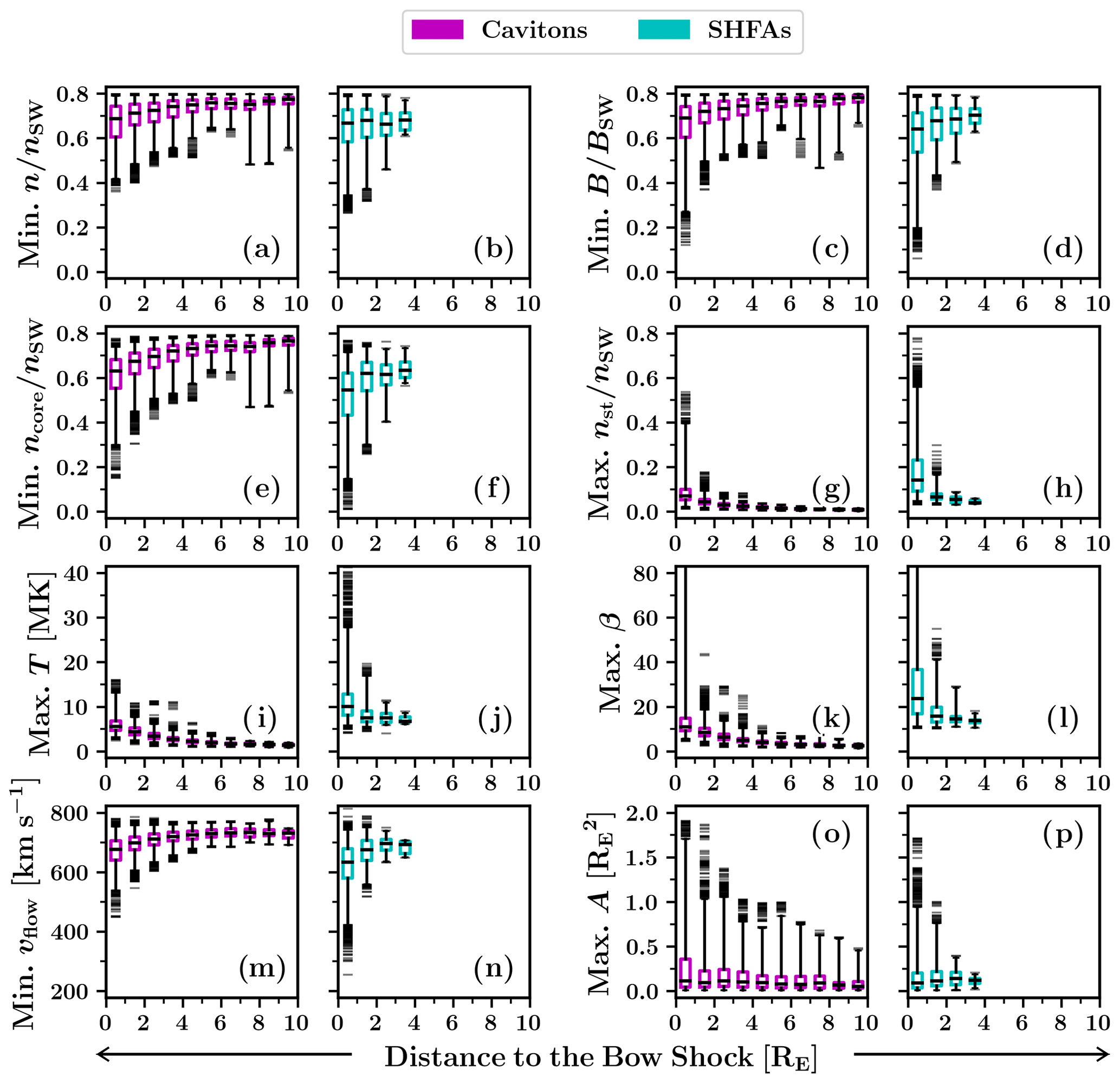
Figure 6Box-and-whiskers plots showing the variation of the tracked transients' physical properties with the distance from the bow shock (along the IMF direction). Each box covers an interval of 1 RE, showing the interquartile data range that contains 50 % of the data around the median, which is shown as a black horizontal line. The whiskers extend to 1 %/99 % of the data, with outliers displayed as horizontal lines.

3.3 Variation of physical properties with the location in the foreshock
We have studied the physical properties of the tracked transients for possible dependencies on the transients' location relative to the bow shock. In Fig. 6 and 7, we present two series of box-and-whiskers plots showing how the properties listed in Table 1 vary with the distance from the bow shock (along the IMF direction) and the nose angle (as defined in the previous section). We compare the variation of the properties of cavitons and SHFAs in side-by-side plots. The data shown contains the properties' extrema from each time step of the tracked transients' lifetimes (as opposed to overall extrema in Table 1), which we categorise into cavitons and SHFAs depending on the type at each time step.
Figure 6 shows that when cavitons and SHFAs are located close to the bow shock, they generally tend to have stronger features, such as larger decreases in the proton number density (Fig. 6a, b, e and f), magnetic field magnitude (Fig. 6c and d), and bulk flow speed (Fig. 6m and n) and larger increases in the proton temperature (Fig. 6i and j). These features are more pronounced inside SHFAs compared to cavitons. Far from the shock, the density/magnetic depressions inside cavitons are mostly shallow. The suprathermal proton number density (Fig. 6g and h) displays a sharp increase at 1 RE from the bow shock, which is also manifested inside SHFAs as an increase in the proton temperature and a decrease in the bulk flow speed. The low amount of suprathermals beyond 1 RE suggests that the accumulation of suprathermals occurs principally very close to the bow shock. Figure 6o and p demonstrate that the maximum areas of the observed transients increase towards the bow shock, but the low median areas ( ) indicate that transients are generally small at all distances. There appears to be no significant difference between the size distributions of cavitons and SHFAs.
Figure 7 suggests that there is no single trend controlling the properties of cavitons and SHFAs as the nose angle varies. A notable feature at the flank of the bow shock at nose angles ≳80∘ is the presence of prominent transients in the upper/lower quartiles of the data, especially visible in the magnetic field magnitude, solar wind core/suprathermal proton number density, β, bulk flow speed and area. Further analysis shows that these transients are a result of several transients merging together. The region where these transients are found coincides with the region of most abundant caviton formation (Fig. 5b), which provides suitable conditions for mergers between transients. Using the same simulation run as we have used in this work, Blanco-Cano et al. (2018) previously reported on the formation of a large magnetosheath cavity at the flank of the bow shock in response to several SHFAs arriving at the shock. Our statistical results further illustrate that for an IMF oriented at a 45∘ cone angle, the flank of the bow shock is a favourable region for the formation of large transients, which can in turn lead to the formation of magnetosheath cavities and erosion of the bow shock. The large transients resulting from mergers can have complex shapes (see Fig. 1), which may also explain the irregular shapes of some of the cavitons seen in multi-spacecraft observations (Kajdič et al., 2011).
Apart from the large transients present at the flank of the bow shock, the properties of cavitons in the interquartile data range appear uniform, and we do not find evidence of significant variation in cavitons' properties with the nose angle. At the flank of the bow shock, we find some large cavitons with high suprathermal counts which are not classified as SHFAs possibly due to their size, as our SHFA criterion requires β>10 in at least 60 % of a transient's cells. Such situation could arise from a merger between a caviton and an SHFA, resulting to the new transient having a high suprathermal count and a low percentage of cells with β>10. For the properties of SHFAs, we observe a clear nose angle dependence in the proton temperature, showing increasing values towards the bow shock nose. This temperature increase results from the backstreaming suprathermal ion population having larger field-aligned velocities near the foreshock edge, leading to larger relative motion with respect to the solar wind near the shock nose. Due to the ambiguity in the variation of other SHFA properties, we repeated our analysis using only transients that are not involved in mergers (not shown). This way, in addition to the proton temperature and β increasing towards the bow shock nose, we found a similar but less distinctive trend in the bulk flow speed, which shows decreasing values towards the bow shock nose. This decrease is likely similar to the temperature increase near the shock nose, caused by the increasing relative motion between the solar wind and the suprathermal population. We did not find signs of notable nose angle dependence in other properties of SHFAs.
3.4 Transient propagation
Our method of tracking cavitons and SHFAs has allowed us to measure the propagation velocities of the transients in a straightforward manner. First, we have calculated the lifetimes of the transients, which range between 0.5–217.5 s with an average lifetime of 20.1 s. Then, we have calculated the distances travelled by the transients by following the position of each transient's magnetic field minimum. The average overall distance travelled by a transient is 1.94 RE, with an average displacement of −1.88 RE in the x direction (Earth-Sun direction) and −0.40 RE in the z direction (out-of-ecliptic direction). Thus, on average, the motion of the transients in the simulation frame of reference is directed anti-sunward and southward. Furthermore, we find transient motion in the northward and sunward directions to be negligible. Since the solar wind in our simulation run flows along the x axis, any out-of-ecliptic motion of the transients is not due to the solar wind motion.
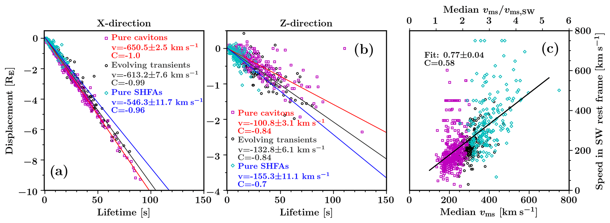
Figure 8(a, b) Scatterplots of the lifetimes of the transients against their displacements in the x direction and the z direction. Linear fits in each panel estimate the propagation velocities for different transient types, including the standard error of the slope of the fit and the Pearson correlation coefficient C. (c) Scatterplot of the over-lifetime median magnetosonic speeds vms inside the transients against the solar wind rest frame propagation speeds of the transients.
In Fig. 8a and b, we have plotted the lifetimes of the transients against their over-the-lifetime displacements in the x direction (Fig. 8a) and the z direction (Fig. 8b). In each direction, we have made linear fits that estimate the propagation velocities of the transients in the simulation frame of reference. To limit the effects of transient interaction and deformation, we have omitted interacting (splitting, merging) transients from Fig. 8. We have calculated separate fits for pure cavitons (N=446), pure SHFAs (N=202) and evolving transients (N=198) to highlight differences between different transient types.
In the x direction, pure cavitons propagate at the greatest velocity, which we estimate to be km s−1. The x directional propagation velocity of pure SHFAs is notably slower, at km s−1, and the transition from cavitons to SHFAs is highlighted by the intermediate propagation velocity of evolving transients ( km s−1). We find excellent correlation between the lifetime and the displacement in the x direction for all transient types, showing that the motion of the transients is uniform as they are advected by the solar wind towards the bow shock. Furthermore, we find that all transient types show x directional propagation velocities that are slower than the solar wind (−750 km s−1), indicating that all transient types have a sunward-directed velocity component in the solar wind rest frame. Accordingly, the x-directional propagation velocities in the solar wind rest frame are ∼99 km s−1 for pure cavitons, ∼204 km s−1 for pure SHFAs and ∼137 km s−1 for evolving transients. In the z direction, pure cavitons have the slowest (southward directed) propagation velocity at km s−1, while pure SHFAs have the fastest propagation velocity at km s−1. Evolving transients again display an intermediate propagation velocity ( km s−1). We note that in the solar wind rest frame, the trends in the z and x directions are similar, with cavitons propagating slower than SHFAs in both directions.
Based on the fits calculated in Fig. 8a and b, we find a total solar wind rest frame propagation velocity of ∼142 km s−1 for pure cavitons, ∼256 km s−1 for pure SHFAs and ∼ 191 km s−1 for evolving transients. The solar wind rest frame propagation of pure cavitons is directed at a sunward and southward angle of ∼45.4∘, indicating that the propagation approximately follows the IMF direction (45∘). We find a similar propagation angle for evolving transients (∼44.1∘), while the propagation is somewhat more sunward oriented for pure SHFAs (∼37.3∘).
To understand the notably different propagation velocities of cavitons and SHFAs, we investigated the relationship between the propagation velocity of the transients and the magnetosonic speed in the foreshock. In Fig. 8c, we have plotted the over-lifetime median values of the magnetosonic speeds measured at the centres of the transients (which we take to be the magnetic minima) against the solar wind rest frame propagation speeds of the transients. Based on visual inspection, we conclude that the magnetosonic speed has similar values inside the transients and in their surroundings, and thus we consider the magnetosonic speeds measured inside the transients to be representative of the surrounding medium.
The results presented in Fig. 8c suggest that the solar wind rest frame propagation speed of the transients increases in concert with the local magnetosonic speed. We find that there is an increase in the magnetosonic speed near the bow shock, leading to SHFAs having a larger propagation speed in the solar wind rest frame compared to cavitons. A linear fit in Fig. 8c estimates the solar wind rest frame propagation speed of the transients to be ∼0.77vms, with vms being the local magnetosonic speed. However, we note that this is a crude estimate, as we have used a temporal median value of the magnetosonic speed and large variation is present in the propagation speeds of the transients. We find that the poor correlation coefficient (C=0.58) in Fig. 8c is in part due to the presence of small, short-lived transients for which the propagation speed may attain very large values (≳400 km s−1). We repeated our analysis using only transients which have a minimum lifetime of 5 s (not shown), and obtained a linear fit with a similar slope (0.77±0.03) and an increased correlation coefficient (C=0.72).
Our choice for the criterion which we use to separate cavitons and SHFAs (SHFAs must have β>10 in at least 60 % of transient cells) appears to be suitable, since we are able to reproduce the characteristics of SHFAs established in existing literature (e.g., Zhang et al., 2013; Omidi et al., 2013), including higher amounts of suprathermal ions, higher temperatures and lower bulk flow speeds inside SHFAs compared to cavitons and the surrounding foreshock. The usage of β however poses some challenges, as the magnetic field magnitude B could influence the transient classification. For example, transients with low B might be classified as SHFAs, explaining the slightly larger mean depletions inside SHFAs compared to cavitons. This does not however appear to be the case, since all SHFAs in our study have a maximum temperature above the mean maximum temperature inside cavitons (Table 1, Fig. 2d), indicating that the larger depletions are associated with an actual increase in temperature rather than a misclassification. To assess the impact of B on β, we compare the thermal pressure P and the reciprocal of the magnetic pressure when B reaches its minimum inside the tracked transients. Comparing the pressures normalised by their input solar wind values shows that the relative increase in P is larger than the relative increase in in 96.8 % of the cases, with the increase in P being 3.9 times as large as the increase in on average. Hence, we conclude that B does not have a statistically significant impact on our transient classification.
While β was chosen as the SHFA criterion in order to not make explicit assumptions on the level of heating/bulk flow deflection inside the transients, we note that a suitable T-based criterion (≳7 MK for SHFAs) would yield similar results. As we observe considerable overlap between cavitons and SHFAs in terms of the bulk flow speed vflow, setting a condition to account both for T and vflow is not straightforward. The low level of bulk flow deflection inside a number of SHFAs suggests that the evolution of cavitons into SHFAs occurs gradually, and there is a proto-SHFA stage in the evolution, during which the transients may exhibit heating and only little bulk flow deflection.
In accordance with Cluster spacecraft observations (Kajdič et al., 2013, 2017), we find the decreases in the proton number density and magnetic field magnitude inside cavitons to be well correlated. The correlation coefficient between these quantities inside cavitons is similar in spacecraft statistics of Kajdič et al. (2017) (C=0.85) and our study (C=0.79). These decreases have weaker correlation inside SHFAs, which is apparent in both spacecraft statistics (C=0.30) and our results (C=0.57). While the weak correlation in spacecraft observations may be in part due to low statistics (N=19), our results suggest that the weak correlation compared to cavitons is caused by the presence of suprathermals, which can counter the decrease in the total proton number density and lead to uneven decreases in the number density and magnetic field magnitude.
The Cluster statistics of Kajdič et al. (2017) demonstrated that SHFAs contain larger density and magnetic field magnitude depletions than cavitons, and our results show agreement with this notion. However, the depletions in our simulation run appear shallow compared to spacecraft observations. In our simulation run, the average maximum decrease in the proton number density (magnetic field magnitude) from its ambient solar wind value is 28 % (28 %) inside cavitons and 36 % (39 %) inside SHFAs. In the spacecraft statistics of Kajdič et al. (2017), the average decreases of the density and magnetic field magnitude are 50 % inside cavitons and 90 % inside SHFAs. The smaller depletions found in our simulation are in part due to our automated transient detection method, which leads to many shallow transients being selected into our statistical sample. These may not be easily visually identifiable in spacecraft time series, and might be discarded by the more stringent selection criteria used in observations. We assessed the impact of the small transients on the calculation of the average density and magnetic field depletions by recalculating the average values using only transients that have a maximum area of at least 0.5 over lifetime (N=75). In this manner, we found notable increases in the average depletions, with the average maximum decrease for the proton number density (magnetic field magnitude) being 44 % (45 %) for cavitons and 55 % (62 %) for SHFAs. The depths of the transients in our simulation run may also be affected by our method of measuring the depths directly from the input solar wind parameters, which do not fully represent the varying conditions in the foreshock. This could possibly lead to the depths of the transients being underestimated.
Similarly, the sizes of the transients in our simulation appear small compared to those found in spacecraft observations. Using Cluster data, Kajdič et al. (2013) estimated the average caviton extent to be ∼4.6 RE for a set of 92 observations. While we have directly measured the areas of the transients in our simulation as opposed to calculating the transient extent in one spatial dimension like in the spacecraft data, the average maximum and overall maximum areas we found (0.16 and 1.91 , respectively) indicate a clear size difference. This discrepancy is likely not due to different solar wind conditions in our simulation and the spacecraft observations. According to Omidi et al. (2014b), the size of the transients should increase with Alfvén Mach number MA. In our simulation, we have MA=6.9, which is similar to the average Alfvén Mach number during the caviton observations of Kajdič et al. (2013) (〈MA〉=6.5, with MA ranging between ). Instead, we identify two effects that may contribute to the difference in the sizes of the transients. First, the sizes could be affected by our solar wind-based transient detection criteria in the same manner as the decreases in density and magnetic field, leading to the transients' sizes to be underestimated. Second, Kajdič et al. (2013) have included the rims of enhanced density/magnetic field magnitude associated with cavitons in the calculated extents. This is not done in our study, since our caviton detection criteria only account for the depressions inside the transients. In the first Vlasiator study of cavitons and SHFAs, Blanco-Cano et al. (2018) noted that these rims are not as prominent in Vlasiator as in spacecraft data. This is believed to be an effect of the spatial resolution of the simulation, which can limit the steepening of ULF waves (Pfau-Kempf et al., 2018), and could also affect the growth of cavitons and SHFAs.
We find overall good agreement between our study and the spacecraft statistics of Kajdič et al. (2017) regarding the locations of cavitons and SHFAs relative to the bow shock. Like Kajdič et al. (2017), we have measured the transients' distances from the bow shock along the IMF direction. In the spacecraft statistics, cavitons and SHFAs have been observed within 9 and 6 RE from the bow shock, respectively. In our simulation run, 99 % of all caviton formation takes place within 11 RE from the bow shock, while all SHFAs are found within 4 RE from the shock. It is noteworthy that the Cluster spacecraft used in the observations of Kajdič et al. (2017) are on an orbit that keeps the spacecraft near the bow shock, which may lead to fewer observations further away from the shock. We also note that the spacecraft statistics span a long time period with varying solar wind/IMF conditions, while our single simulation run has a constant solar wind and IMF. It is possible that the distance measurement is affected by the orientation of the IMF, and that the extents of the caviton/SHFA regions change with the solar wind/IMF conditions. Investigating the influence of parameters such as Alfvén Mach number and IMF cone angle on the extent of the caviton/SHFA region is a possible topic for a future study.
Our results indicate that the accumulation of suprathermals inside SHFAs is closely tied to the transients' distance from the bow shock. This is exemplified by the fact that we see a simultaneous onset of copious SHFA formation and caviton-to-SHFA evolution at ∼2 RE from the bow shock (as measured along the IMF direction), occurring at roughly the same distance at all parts of the quasi-parallel bow shock. Most notably, we observe a significant jump in the suprathermal proton number density, temperature and the level of bulk flow deflection at ≲1 RE from the shock inside both cavitons and SHFAs. The enhancements inside cavitons are comparable with those in the surrounding foreshock (as evaluated via troughs of foreshock fluctuations), which displays a general increase in the suprathermal density, temperature and level of bulk flow deflection near the shock. The enhancements inside SHFAs are larger than in the surrounding foreshock, which suggests that there is accumulation of suprathermals inside the SHFAs rather than only a change in the general foreshock conditions. Overall, we also see larger decreases inside the transients in the proton number density and magnetic field magnitude near the bow shock, which is in agreement with prior numerical studies of cavitons (Blanco-Cano et al., 2009, 2011).
The angular distance from the Sun–Earth line (i.e., the nose angle) appears to affect the formation and the properties of SHFAs. We find our results to be in good agreement with the findings of Omidi et al. (2014b), who studied the dependence of SHFAs' properties on the distance from the Sun–Earth line using global hybrid simulations with various Alfvén Mach numbers and IMF orientations. Both our study and the study of Omidi et al. (2014b) find that the amount of SHFAs decreases towards the flank of the bow shock. The decreasing SHFA formation rate is likely influenced by the angle θBn between the shock normal and the IMF direction, as the rate in our simulation peaks at θBn∼0–10∘ and decreases steadily at larger angles. The decreasing amount of SHFAs at the bow shock flank is contrasted by the abundant formation of cavitons there, which emphasises that there is no decline in the transient formation rate at the flank but the transients there generally undergo lesser heating/evolution compared to the subsolar region. Similar to Omidi et al. (2014b), we clearly observe that the temperature inside SHFAs increases towards the bow shock nose. As we noted in Sect. 3.3, the temperature increase is linked to larger relative motion between the backstreaming suprathermal protons and the incoming solar wind near the shock nose. The temperature inside the SHFAs in our simulation run (MA=6.9) increases to ∼8–60 TSW, which is in good agreement with the values obtained by Omidi et al. (2014b) for different Alfvén Mach numbers (∼2–20 TSW for MA=5 and ∼5–160 TSW for MA=11). Omidi et al. (2014b) also noted a clear dependence on the distance from the Sun–Earth line in the bulk flow speed inside SHFAs that favours smaller speeds near the shock nose when the Alfvén Mach number is large (MA=11). We also find some evidence of larger reductions in the bulk flow speed inside SHFAs near the bow shock nose, although we do not see as clear variation with the distance from the Sun–Earth line as in the temperature. This could be due to the smaller Alfvén Mach number in our simulation run.
In agreement with previous studies of cavitons, the transients in our simulation exhibit sunward motion in the solar wind rest frame, while they propagate anti-sunward in the simulation frame. Our estimates for the solar wind rest frame propagation speeds of the transients ( km s−1) are comparable to those found in multi-spacecraft measurements. Kajdič et al. (2011) used a simple timing method to calculate the sunward propagation speeds of two cavitons (120, 188 km s−1), while Wang et al. (2020) used a variety of multipoint analysis methods to calculate the velocities of 12 cavitons (≲300 km s−1). Our results suggest that SHFAs propagate at a faster solar wind rest frame speed than cavitons due to an increase in the magnetosonic speed near the bow shock. We attribute this increase in the magnetosonic speed to an enhanced pressure/temperature near the shock, leading to an increased sound speed. On the other hand, the Alfvén speed does not show significant dependence on the bow shock distance but instead fluctuates with the wave activity in the foreshock. Due to this, estimating the Alfvén speed in the foreshock is difficult. With respect to the ambient solar wind, the solar wind rest frame motion of the transients in our simulation run is super-Alfvénic (1.3vA,SW for pure cavitons, 2.4vA,SW for pure SHFAs), agreeing with earlier reports of super-Alfvénic motion of cavitons (Blanco-Cano et al., 2011; Wang et al., 2020).
In accordance with the results of Wang et al. (2020), our results indicate that cavitons propagate in the direction of the IMF. However, in order to reach definite conclusions on the propagation direction, multiple simulation runs with different IMF orientations should be used. We find that compared to cavitons, the propagation of SHFAs is somewhat more sunward oriented (for an IMF cone angle of 45∘). This may be due to the conditions near the bow shock, where the propagation of SHFAs is influenced by the highly perturbed flow/magnetic field. Accumulation of ions that have been specularly reflected from the bow shock could also affect the propagation of SHFAs by introducing a velocity component parallel to the local shock normal direction, which near the nose of the bow shock could explain the more sunward oriented propagation of SHFAs.
In this work, we have statistically studied cavitons and SHFAs in Earth's foreshock using a global hybrid-Vlasov simulation run conducted in the noon–midnight meridional plane. Our simulation corresponds to fast solar wind conditions, having an Alfvén Mach number MA=6.9 and an IMF cone angle of 45∘. We have found that under such conditions, cavitons and SHFAs are a common occurrence in the foreshock, with ∼1–4 new transients forming every second and 29–72 transients populating the foreshock in the noon–midnight meridional plane at any given time. We find cavitons to be more numerous than SHFAs, with cavitons making up ∼75 % of the simultaneously observed transients on average.
The properties of cavitons and SHFAs in our simulation are in good overall agreement with the findings of prior numerical and observational studies. We find the depressions of the plasma density and magnetic field magnitude to be well-correlated inside cavitons, while the correlation is reduced inside SHFAs due to their copious accumulation of suprathermal protons. On average, the depressions are larger inside SHFAs. Clear correspondence is found between the amount of suprathermals and the level of heating and bulk flow speed reduction inside SHFAs. While the temperatures inside SHFAs are notably higher than inside cavitons, a gradual transition between cavitons and SHFAs is seen for the reduction in the bulk flow speed, with many transients exhibiting moderate speed reductions. This suggests an intermediate stage in the caviton-to-SHFA evolution, in which the transients are heated but have minor bulk flow deflections. The only clear discrepancy regarding the properties of cavitons/SHFAs between our simulation and spacecraft observations is seen in the transients' sizes and the depths of their density/magnetic depressions, which are smaller in our simulation than in observations. This may be due to the differing methods used in measuring the extents/depths of the transients or the resolution of our simulation being a limiting factor for the growth of the transients.
We find continuous formation of cavitons extending up to ∼11 RE from the bow shock (as measured along the IMF direction). The caviton formation region attains its largest extent deep in the foreshock, showing gradual expansion from the bow shock nose towards the flank of the shock. The formation most likely extends beyond the boundary of our simulation domain, which prevents us from determining the full extent of the caviton formation region. Cavitons are principally found to evolve into SHFAs within ∼2 RE from the bow shock, where SHFAs are also commonly found forming independently; ∼55 % of the observed SHFAs evolve from cavitons, while the rest form independently. Not all cavitons in our run undergo evolution, with only roughly a third of all cavitons turning into SHFAs. SHFAs emerge at similar distances in all parts of the foreshock, although the rate of SHFA formation/caviton evolution declines towards the flank of the bow shock.
The properties of cavitons and SHFAs show some dependence on the transients' position relative to the bow shock. We have found that there are overall increases in the depth of the density/magnetic depressions and the level of heating and bulk flow speed reduction inside transients as their distance to the bow shock decreases. The number density of suprathermal protons inside the transients is generally low until ≲1 RE from the shock, showing that the accumulation of suprathermals is concentrated near the bow shock. The SHFAs' distance from the Sun–Earth line has a clear effect on the temperature inside them, with higher temperatures found near the bow shock nose. There is a similar, but weaker dependency for the bulk flow speed inside SHFAs, with lower speeds near the nose. The distance from the Sun–Earth line does not appear to have any direct effect on the properties of cavitons, but our results suggest that mergers between transients can lead to the formation of large transients deep in the foreshock where the formation of cavitons is most abundant.
The transients in our simulation run propagate sunward in the solar wind rest frame of reference, but they are advected anti-sunward in the simulation frame of reference by the solar wind. The propagation also has an out-of-ecliptic component, which is directed southward in our simulation run where the IMF also has a southward component. We have found that the propagation of cavitons in the solar wind rest frame is aligned with the direction of the IMF, while SHFAs exhibit slightly more sunward oriented propagation. We find that SHFAs have a greater solar wind rest frame speed than cavitons, which is related to an increase in the magnetosonic speed near the bow shock. We find an approximate solar wind rest frame transient propagation speed of ∼0.77vms, with vms being the local magnetosonic speed. The solar wind rest frame propagation speed of the transients exceeds the Alfvén speed vA,SW in the ambient solar wind, with a speed of 1.3vA,SW for cavitons and 2.4vA,SW for SHFAs.
Our study has presented a comprehensive picture of cavitons and SHFAs in Earth's foreshock and has demonstrated the usefulness of global hybrid-Vlasov simulations in complementing spacecraft observations of foreshock phenomena. Topics especially suited for global simulations include the propagation and the evolution of foreshock transients, which in spacecraft studies typically require the usage of multi-spacecraft missions. In future numerical studies, multiple simulation runs with different solar wind conditions could be used to study the effect of parameters such as the Alfvén Mach number and the IMF cone angle on the formation, propagation and evolution of cavitons and SHFAs.
Vlasiator (http://www.helsinki.fi/en/researchgroups/vlasiator/, Palmroth, 2020) is distributed under the GPL-2 open source license at https://doi.org/10.5281/zenodo.3640594 (Palmroth and the Vlasiator team, 2020). Vlasiator uses a data structure developed in-house (https://github.com/fmihpc/vlsv/, Sandroos, 2019). The Analysator software (https://github.com/fmihpc/analysator/, Battarbee and the Vlasiator team, 2020) was used to produce the presented figures. The run described here takes several terabytes of disk space and is kept in storage maintained within the CSC – IT Center for Science. Data presented in this paper can be accessed by following the data policy on the Vlasiator web site.
VT wrote the first draft of the manuscript and performed the data analysis. LT and MB provided guidance in analysing and interpreting the results. JS developed the tracking methodology which was adapted by VT for this study. XBC led the work that served as a starting point for this study, and helped with interpreting the results. MP is the PI of the Vlasiator model and MB, UG and YPK ran the Vlasiator run used in this study. All coauthors (including MA, MD, MG, AJ and KP) participated in the discussion of the results and the improvement of the article.
The authors declare that they have no conflict of interest.
Publisher's note: Copernicus Publications remains neutral with regard to jurisdictional claims in published maps and institutional affiliations.
The CSC-IT Center for Science in Finland is acknowledged for the Sisu supercomputer pilot usage and Grand Challenge award, leading to the results presented here.
The development of Vlasiator has been supported by the European Research Council (grant nos. 200141-QuESpace and 682068-PRESTISSIMO). The work leading to these results has been carried out in the Finnish Centre of Excellence in Research of Sustainable Space (Academy of Finland, grant no. 312351). The work of Vertti Tarvus and Lucile Turc is supported by the Academy of Finland (grant nos. 322544 and 328893).
Open-access funding was provided by the Helsinki University Library.
This paper was edited by Jonathan Rae and reviewed by Hui Zhang and Martin Archer.
Archer, M. O., Turner, D. L., Eastwood, J. P., Schwartz, S. J., and Horbury, T. S.: Global impacts of a Foreshock Bubble: Magnetosheath, magnetopause and ground-based observations, Planet. Space Sci., 106, 56–66, https://doi.org/10.1016/j.pss.2014.11.026, 2015. a
Battarbee, M. and the Vlasiator team: Analysator: python analysis toolkit, Github repository, available at: https://github.com/fmihpc/analysator/, last access: 16 October 2020. a
Battarbee, M., Ganse, U., Pfau-Kempf, Y., Turc, L., Brito, T., Grandin, M., Koskela, T., and Palmroth, M.: Non-locality of Earth's quasi-parallel bow shock: injection of thermal protons in a hybrid-Vlasov simulation, Ann. Geophys., 38, 625–643, https://doi.org/10.5194/angeo-38-625-2020, 2020. a
Billingham, L., Schwartz, S. J., and Wilber, M.: Foreshock cavities and internal foreshock boundaries, Planet. Space Sci., 59, 456–467, https://doi.org/10.1016/j.pss.2010.01.012, 2011. a
Blanco-Cano, X., Omidi, N., and Russell, C. T.: Global hybrid simulations: Foreshock waves and cavitons under radial interplanetary magnetic field geometry, J. Geophys. Res.-Space, 114, A01216, https://doi.org/10.1029/2008JA013406, 2009. a, b, c, d
Blanco-Cano, X., Kajdič, P., Omidi, N., and Russell, C. T.: Foreshock cavitons for different interplanetary magnetic field geometries: Simulations and observations, J. Geophys. Res.-Space, 116, A09101, https://doi.org/10.1029/2010JA016413, 2011. a, b, c, d, e
Blanco-Cano, X., Battarbee, M., Turc, L., Dimmock, A. P., Kilpua, E. K. J., Hoilijoki, S., Ganse, U., Sibeck, D. G., Cassak, P. A., Fear, R. C., Jarvinen, R., Juusola, L., Pfau-Kempf, Y., Vainio, R., and Palmroth, M.: Cavitons and spontaneous hot flow anomalies in a hybrid-Vlasov global magnetospheric simulation, Ann. Geophys., 36, 1081–1097, https://doi.org/10.5194/angeo-36-1081-2018, 2018. a, b, c, d, e, f
Chu, C., Zhang, H., Sibeck, D., Otto, A., Zong, Q., Omidi, N., McFadden, J. P., Fruehauff, D., and Angelopoulos, V.: THEMIS satellite observations of hot flow anomalies at Earth's bow shock, Ann. Geophys., 35, 443–451, https://doi.org/10.5194/angeo-35-443-2017, 2017. a
Daldorff, L. K. S., Tóth, G., Gombosi, T. I., Lapenta, G., Amaya, J., Markidis, S., and Brackbill, J. U.: Two-way coupling of a global Hall magnetohydrodynamics model with a local implicit particle-in-cell model, J. Comput. Phys., 268, 236–254, https://doi.org/10.1016/j.jcp.2014.03.009, 2014. a
Eastwood, J. P., Lucek, E. A., Mazelle, C., Meziane, K., Narita, Y., Pickett, J., and Treumann, R. A.: The Foreshock, Space Sci. Rev., 118, 41–94, https://doi.org/10.1007/s11214-005-3824-3, 2005. a
Fuselier, S. A.: Ion distributions in the Earth's foreshock upstream from the bow shock, Adv. Space Res., 15, 43–52, https://doi.org/10.1016/0273-1177(94)00083-D, 1995. a
Greenstadt, E. W., Le, G., and Strangeway, R. J.: ULF waves in the foreshock, Adv. Space Res., 15, 71–84, https://doi.org/10.1016/0273-1177(94)00087-H, 1995. a
Hoilijoki, S., Ganse, U., Sibeck, D. G., Cassak, P. A., Turc, L., Battarbee, M., Fear, R. C., Blanco-Cano, X., Dimmock, A. P., Kilpua, E. K. J., Jarvinen, R., Juusola, L., Pfau-Kempf, Y., and Palmroth, M.: Properties of Magnetic Reconnection and FTEs on the Dayside Magnetopause With and Without Positive IMF Bx Component During Southward IMF, J. Geophys. Res.-Space, 124, 4037–4048, https://doi.org/10.1029/2019JA026821, 2019. a
Hoppe, M. M., Russell, C. T., Frank, L. A., Eastman, T. E., and Greenstadt, E. W.: Upstream hydromagnetic waves and their association with backstreaming ion populations – ISEE 1 and 2 observations, J. Geophys. Res., 86, 4471–4492, https://doi.org/10.1029/JA086iA06p04471, 1981. a
Kajdič, P., Blanco-Cano, X., Omidi, N., and Russell, C. T.: Multi-spacecraft study of foreshock cavitons upstream of the quasi-parallel bow shock, Planet. Space Sci., 59, 705–714, https://doi.org/10.1016/j.pss.2011.02.005, 2011. a, b, c, d, e
Kajdič, P., Blanco-Cano, X., Omidi, N., Meziane, K., Russell, C. T., Sauvaud, J.-A., Dandouras, I., and Lavraud, B.: Statistical study of foreshock cavitons, Ann. Geophys., 31, 2163–2178, https://doi.org/10.5194/angeo-31-2163-2013, 2013. a, b, c, d, e, f, g, h, i, j, k, l, m
Kajdič, P., Blanco-Cano, X., Omidi, N., Rojas-Castillo, D., Sibeck, D. G., and Billingham, L.: Traveling Foreshocks and Transient Foreshock Phenomena, J. Geophys. Res.-Space, 122, 9148–9168, https://doi.org/10.1002/2017JA023901, 2017. a, b, c, d, e, f, g, h, i, j, k, l, m
Kempf, Y., Pokhotelov, D., Gutynska, O., Wilson, Lynn B., I., Walsh, B. M., von Alfthan, S., Hannuksela, O., Sibeck, D. G., and Palmroth, M.: Ion distributions in the Earth's foreshock: Hybrid-Vlasov simulation and THEMIS observations, J. Geophys. Res.-Space, 120, 3684–3701, https://doi.org/10.1002/2014JA020519, 2015. a
Lin, Y.: Global-scale simulation of foreshock structures at the quasi-parallel bow shock, J. Geophys. Res.-Space, 108, 1390, https://doi.org/10.1029/2003JA009991, 2003. a
Lin, Y. and Wang, X. Y.: Three-dimensional global hybrid simulation of dayside dynamics associated with the quasi-parallel bow shock, J. Geophys. Res.-Space, 110, A12216, https://doi.org/10.1029/2005JA011243, 2005. a
Lucek, E. A., Horbury, T. S., Balogh, A., Dand ouras, I., and RèMe, H.: Cluster observations of hot flow anomalies, J. Geophys. Res.-Space, 109, A06207, https://doi.org/10.1029/2003JA010016, 2004. a
Omidi, N.: Formation of cavities in the foreshock, in: Turbulence and Nonlinear Processes in Astrophysical Plasmas, edited by Shaikh, D. and Zank, G. P., vol. 932 of American Institute of Physics Conference Series, 181–190, https://doi.org/10.1063/1.2778962, 2007. a
Omidi, N., Zhang, H., Sibeck, D., and Turner, D.: Spontaneous hot flow anomalies at quasi-parallel shocks: 2. Hybrid simulations, J. Geophys. Res.-Space, 118, 173–180, https://doi.org/10.1029/2012JA018099, 2013. a, b
Omidi, N., Sibeck, D., Gutynska, O., and Trattner, K. J.: Magnetosheath filamentary structures formed by ion acceleration at the quasi-parallel bow shock, J. Geophys. Res.-Space, 119, 2593–2604, https://doi.org/10.1002/2013JA019587, 2014a. a
Omidi, N., Zhang, H., Chu, C., Sibeck, D., and Turner, D.: Parametric dependencies of spontaneous hot flow anomalies, J. Geophys. Res.-Space, 119, 9823–9833, https://doi.org/10.1002/2014JA020382, 2014b. a, b, c, d, e, f, g, h, i
Omidi, N., Berchem, J., Sibeck, D., and Zhang, H.: Impacts of spontaneous hot flow anomalies on the magnetosheath and magnetopause, J. Geophys. Res.-Space, 121, 3155–3169, https://doi.org/10.1002/2015JA022170, 2016. a, b
Palmroth, M.: Vlasiator, Web site, available at: https://www.helsinki.fi/en/researchgroups/vlasiator/, last access: 16 October 2020. a
Palmroth, M. and the Vlasiator team: Vlasiator: hybrid-Vlasov simulation code, version 5.0, Zenodo [code], https://doi.org/10.5281/zenodo.3640594 (last access: 12 October 2021), 2020. a
Palmroth, M., Ganse, U., Pfau-Kempf, Y., Battarbee, M., Turc, L., Brito, T., Grandin, M., Hoilijoki, S., Sandroos, A., and von Alfthan, S.: Vlasov methods in space physics and astrophysics, Living Reviews in Computational Astrophysics, 4, 1, https://doi.org/10.1007/s41115-018-0003-2, 2018. a, b
Pfau-Kempf, Y., Battarbee, M., Ganse, U., Hoilijoki, S., Turc, L., von Alfthan, S., Vainio, R., and Palmroth, M.: On the importance of spatial and velocity resolution in the hybrid-Vlasov modeling of collisionless shocks, Front. Phys., 6, 44, https://doi.org/10.3389/fphy.2018.00044, 2018. a
Sandroos, A.: VLSV: file format and tools, Github repository, available at: https://github.com/fmihpc/vlsv/ last access: 16 October 2020), 2019. a
Schwartz, S. J.: Hot flow anomalies near the Earth's bow shock, Adv. Space Res., 15, 107–116, https://doi.org/10.1016/0273-1177(95)00025-A, 1995. a
Schwartz, S. J., Chaloner, C. P., Christiansen, P. J., Coates, A. J., Hall, D. S., Johnstone, A. D., Gough, M. P., Norris, A. J., Rijnbeek, R. P., Southwood, D. J., and Woolliscroft, L. J. C.: An active current sheet in the solar wind, Nature, 318, 269–271, https://doi.org/10.1038/318269a0, 1985. a
Schwartz, S. J., Sibeck, D., Wilber, M., Meziane, K., and Horbury, T. S.: Kinetic aspects of foreshock cavities, Geophys. Res. Lett., 33, L12103, https://doi.org/10.1029/2005GL025612, 2006. a, b
Schwartz, S. J., Avanov, L., Turner, D., Zhang, H., Gingell, I., Eastwood, J. P., Gershman, D. J., Johlander, A., Russell, C. T., Burch, J. L., Dorelli, J. C., Eriksson, S., Ergun, R. E., Fuselier, S. A., Giles, B. L., Goodrich, K. A., Khotyaintsev, Y. V., Lavraud, B., Lindqvist, P.-A., Oka, M., Phan, T.-D., Strangeway, R. J., Trattner, K. J., Torbert, R. B., Vaivads, A., Wei, H., and Wilder, F.: Ion Kinetics in a Hot Flow Anomaly: MMS Observations, Geophys. Res. Lett., 45, 11,520–11,529, https://doi.org/10.1029/2018GL080189, 2018. a
Sibeck, D. G., Phan, T. D., Lin, R., Lepping, R. P., and Szabo, A.: Wind observations of foreshock cavities: A case study, J. Geophys. Res.-Space, 107, 1271, https://doi.org/10.1029/2001JA007539, 2002. a
Thomsen, M. F., Gosling, J. T., Bame, S. J., Quest, K. B., Russell, C. T., and Fuselier, S. A.: On the origin of hot diamagnetic cavities near the Earth's bow shock, J. Geophys. Res., 93, 11311–11325, https://doi.org/10.1029/JA093iA10p11311, 1988. a
von Alfthan, S., Pokhotelov, D., Kempf, Y., Hoilijoki, S., Honkonen, I., Sandroos, A., and Palmroth, M.: Vlasiator: First global hybrid-Vlasov simulations of Earth's foreshock and magnetosheath, J. Atmos. Sol.-Terr. Phy., 120, 24–35, https://doi.org/10.1016/j.jastp.2014.08.012, 2014. a, b
Wang, M., Yao, S., Shi, Q., Zhang, H., Tian, A., Degeling, A. W., Zhang, S., Guo, R., Sun, W., Liu, J., Bai, S., Shen, X., Zhu, X., Fu, S., and Pu, Z.: Propagation properties of foreshock cavitons: Cluster observations, Sci. China E, 63, 173–182, https://doi.org/10.1007/s11431-018-9450-3, 2020. a, b, c, d
Wang, S., Zong, Q., and Zhang, H.: Hot flow anomaly formation and evolution: Cluster observations, J. Geophys. Res.-Space, 118, 4360–4380, https://doi.org/10.1002/jgra.50424, 2013. a
Wilson, L. B.: Low Frequency Waves at and Upstream of Collisionless Shocks, Washington DC American Geophysical Union Geophysical Monograph Series, 216, 269–291, https://doi.org/10.1002/9781119055006.ch16, 2016. a
Wilson, L. B., Sibeck, D. G., Breneman, A. W., Le Contel, O., Cully, C., Turner, D. L., Angelopoulos, V., and Malaspina, D. M.: Quantified energy dissipation rates in the terrestrial bow shock: 1. Analysis techniques and methodology, J. Geophys. Res.-Space, 119, 6455–6474, https://doi.org/10.1002/2014JA019929, 2014. a
Zhang, H. and Zong, Q.: Transient Phenomena at the Magnetopause and Bow Shock and Their Ground Signatures, chap. 2, pp. 11–37, American Geophysical Union (AGU), https://doi.org/10.1002/9781119509592.ch2, 2020. a
Zhang, H., Sibeck, D. G., Zong, Q. G., Omidi, N., Turner, D., and Clausen, L. B. N.: Spontaneous hot flow anomalies at quasi-parallel shocks: 1. Observations, J. Geophys. Res.-Space, 118, 3357–3363, https://doi.org/10.1002/jgra.50376, 2013. a, b, c