the Creative Commons Attribution 4.0 License.
the Creative Commons Attribution 4.0 License.
 | 16 Jun 2021
Even moderate geomagnetic pulsations can cause fluctuations of foF2 frequency of the auroral ionosphere
Nadezda Yagova
Alexander Kozlovsky
Evgeny Fedorov
Olga Kozyreva
The ionosonde at the Sodankylä Geophysical Observatory (SOD; 67∘ N, 27∘ E; Finland) routinely performs vertical sounding once per minute which enables the study of fast ionospheric variations at a frequency of the long-period geomagnetic pulsations Pc5–6/Pi3 (1–5 mHz). Using the ionosonde data from April 2014–December 2015 and colocated geomagnetic measurements, we have investigated a correspondence between the magnetic field pulsations and variations of the critical frequency of radio waves reflected from the ionospheric F2 layer (foF2). For this study, we have developed a technique for automated retrieval of the critical frequency of the F2 layer from ionograms. As a rule, the Pc5–6/Pi3 frequency band fluctuations in foF2 were observed at daytime during quiet or moderately disturbed space weather conditions. In most cases (about 80 %), the coherence between the foF2 variations and geomagnetic pulsations was low. However in some cases (specified as “coherent”) the coherence was as large as γ2≥0.5. The following conditions are favorable for the occurrence of coherent cases: enhanced auroral activity (6 h maximal auroral electrojet (AE) ≥800 nT), high solar wind speed (V>600 km/s), fluctuating solar wind pressure and northward interplanetary magnetic field. In the cases when the coherence was higher at shorter periods of oscillations, the magnetic pulsations demonstrated features typical for the Alfvén field line resonance.
- Article
(6108 KB) - Full-text XML
-
Supplement
(1592 KB) - BibTeX
- EndNote


Ionospheric variations at the frequency corresponding to simultaneous geomagnetic pulsations were observed in the total electron content (TEC) and have been interpreted as a modulation of the ionosphere by magnetospheric processes (e.g., Davies and Hartmann, 1976; Okuzawa and Davies, 1981). Ionospheric modulation at a frequency of Pc3–4 geomagnetic pulsations (6.7–80 mHz) was found at mid and low latitudes (Davies and Hartmann, 1976; Okuzawa and Davies, 1981). Davies and Hartmann (1976) reported on pulsations in TEC, recorded under undisturbed conditions and associated with Pc3–4s on the ground. Later, Okuzawa and Davies (1981) confirmed the correspondence between ground and TEC variations in the Pc3–4 frequency range, but they obtained the maximal probability under disturbed conditions.
Particle precipitation at auroral latitudes is one of the most intensive processes of the magnetosphere–ionosphere coupling. It is modulated by intensive ultralow-frequency (ULF) waves, and this was a topic of numerous studies. Clear features of Pc5 pulsations in the Doppler velocities of the F-layer ionospheric irregularities were found by Ruohoniemi et al. (1991) using coherent-scatter radar observations. Wright et al. (1997) analyzed ionospheric signatures of auroral Pc4–5s with Doppler sounding. They concentrated on large-scale pulsations correlated in the ionosphere and on the ground. These pulsations demonstrated azimuthal wave numbers m typical for ground Pc4-5s and field line resonance (FLR) features. Particle populations responsible for generation of small-scale (high m) waves and their ionospheric signatures were studied by Baddeley et al. (2005). The substorm Pc5 waves with intermediate m registered simultaneously in ion flux in the magnetosphere and in radar observations were reported by Mager et al. (2019). James et al. (2016) showed that the energy of precipitating particles and ULF wave number were controlled by the distance from the substorm epicenter.
Publications devoted to Pc5–6/Pi3 wave signatures in total electron content (TEC) are not numerous. Watson et al. (2015) presented the large-amplitude TEC variations in the Pc5–6 frequency band detected by GPS receivers. They suggested that these TEC variations were associated with the compressional mode of magneto-hydrodynamic (MHD) waves. The corresponding pulsations were also manifested in the magnetic field on the ground with two spectral maxima at about 0.9 and 3.3 mHz. This event was observed in the afternoon after a steep increase of solar wind (SW) dynamic pressure up to almost 20 nPa. It was also followed by a modulation of electron flux measured at the geostationary orbit. An important feature of the observed oscillations was that the amplitude of TEC variations was higher than that found by Pilipenko et al. (2014a), although the geomagnetic pulsations on the ground were not so intensive.
Vorontsova et al. (2016) observed the effect of TEC modulation by ULF waves at low latitudes far away from the resonant L-shells and the zones where kinetic modes can occur due to wave–particle interaction. This has allowed us to identify the observed ULF waves as fast magnetosonic mode. Kozyreva et al. (2019) investigated the Pc5 frequency band oscillations in the ionosonde data at an auroral station and found an intriguing effect of the ionospheric oscillations at a second harmonic of the simultaneously observed geomagnetic pulsations.
Pilipenko et al. (2014a) have found the effect of ionosphere heating in the F-layer by an intense MHD wave at the recovery phase of a magnetic storm. It was not associated with noticeable electron precipitation. The TEC variations in this event were then studied by Pilipenko et al. (2014b), and Pc5-related TEC variations were retrieved. Pilipenko et al. (2014b) suggested several mechanisms of the TEC modulation by ULF waves associated with Pc5 pulsations and estimated the related amplitudes of TEC variations. For some of them, no detectable variations of TEC were found under realistic Pc5 amplitudes. Meanwhile, such mechanisms as Joule heating provide detectable amplitudes for intensive Pc5s.
The efficiency of the TEC modulation by ULF waves depends on the modulation of the particle flux in the magnetosphere. However, long-term measurements at geostationary orbit are available for electrons at energies E>30 keV. A data deficit at lower energies can be partly compensated by numerical modeling. Buchert et al. (1999) modeled variations of ionospheric Hall and Pedersen conductivities associated with ULF modulation of the electron flux at energies of several kiloelectron volts. These results correspond to the E-layer of the ionosphere; i.e., the electron energy is still too high to control foF2 fluctuations. Recently, 6 years of Van Allen Probes measurements confirmed the influence of ULF waves in Pc4 and Pc5 frequency ranges on electrons with energies up to the order of 102 eV with maximum occurrence around L from 5.5 to 7 (Ren et al., 2019).
Watson et al. (2015) showed experimentally that high amplitudes of TEC variations can be observed under lower Pc5–6 amplitudes than it follows from the analysis of ULF wave modulation of the ionosphere without a particle flux modulation.
Thus, a question arises about a statistical relationship between geomagnetic and ionospheric pulsations. Until now, the role of MHD waves in a wide range of amplitudes in variations of foF2 critical frequency has not been studied sufficiently.
In the present paper we attempt to study statistics of the variations of foF2 critical frequency at the Pc5–6/Pi3 frequencies and simultaneous geomagnetic pulsations in the same frequency range.
2.1 Data
Data of the ionosphere sounding were obtained from the Sodankylä Geophysical Observatory (SOD, 67.3∘ N, 26.7∘ E). The SOD ionosonde routinely performs vertical sounding once per minute. A detailed description of the ionosonde can be found in Kozlovsky et al. (2013). The SOD magnetometer is included in the IMAGE magnetometer network (Taskanen, 2009), and data of the three components of the geomagnetic field are available with 10 s sampling rate. For the analysis of the spatial distribution of geomagnetic pulsations, we also use data from another IMAGE magnetometer in Masi (MAS), which is located almost at the same geomagnetic longitude but at a higher latitude (Table 1).
Table 1Coordinates and other parameters of IMAGE stations.
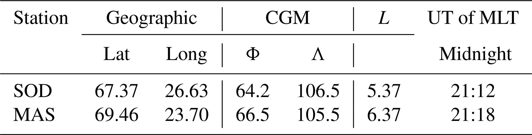
Corrected geomagnetic (CGM) latitude Φ and longitude Λ, apex of the magnetic field line L, and UT of magnetic local midnight are calculated online with http://omniweb.gsfc.nasa.gov/vitmo/cgm.html (last access: 28 April 2021).
The space weather parameters were obtained from the OMNI database at http://cdaweb.gsfc.nasa.gov (last access: 28 April 2021). We used data of the interplanetary magnetic field; speed and dynamic pressure of the solar wind, recalculated to the subsolar point of the magnetosphere (Bargatze et al., 2005); and the indices of geomagnetic storm and auroral activity, namely, the disturbance storm time (Dst) and auroral electrojet (AE) indices. As ULF wave activity the in Pc5–6/Pi3 frequency range depends mostly on the vertical component of the interplanetary magnetic field (IMF BZ), solar wind velocity V, and fluctuations of the solar wind pressure PSW (Baker et al., 2003), these parameters are used for the analysis.

Figure 1Examples ionograms and approximations of F(h) dependence with Eq. (1). foF2 and h1,F1 and F2 approximation parameters are shown in panel (a). Reflection intensity is shown in color in decibel (dB).
We have looked through the ionosonde and SOD magnetometer data from April 2014 through December 2015 and visually selected intervals for further analysis according to the following criteria:
-
The F trace is clearly seen in the ionograms, such that the foF2 critical frequency can be retrieved.
-
Geomagnetic pulsations Pc5–6 or Pi3 are seen in the northward (BX) component, and their peak-to-peak amplitude exceeds 5 nT during at least 2 h during the daytime, between 08:00 and 14:00 UT, corresponding to 11:00–17:00 magnetic local time, MLT, at SOD.
A list of selected intervals is given in Table 2.
Table 2Intervals with foF2 obtained from Eq. (1) checked visually. Years 2014–2015, with DOY representing day of the year.

2.2 foF2 automatic detection from ionograms
Although the visual scaling of the foF2 values from ionograms with clearly identified frequency traces (F traces) is easy, studies of high-frequency variations require scaling of many ionograms, so one needs an automated procedure for that. The difficulties of this procedure are caused by variability of the intensity of reflected signals, background noise, sporadic layers and irregularities, broadcast interference, etc. For these reasons, the techniques of automated foF2 detection can be unstable, even in the cases when visual detection is possible.
Note that the problem of ionospheric density fluctuations involves two different frequency ranges, namely, frequencies of the ionosphere sounding which are about several megahertz and frequencies of geomagnetic and foF2 pulsations in the millihertz range. We use different notations, F and f, for them.
In the present study, we used a method based on the approximation of the F trace in a wide range of altitudes to reduce the influence of gaps and intensity peaks at some frequencies. The F trace (i.e., the curve showing dependence of the frequency of reflected wave on the virtual height of reflection) is characterized by a near-linear growth at low height with gradual transition to saturation at the critical frequency (Fig. 1). The reflection intensity in Fig. 1 is given in decibel (dB), whereas a linear scale (voltage in arbitrary units) is used in the calculation. We approximate this dependence by a Lorentzian function such as
The approximation was made above a starting height h1=235 km. At this altitude F1=F(h1), while F2 is the frequency limit as h→∞. Actually, foF2 is close to F2, but a minor difference between these two values indicates that a nonzero positive derivative in the F(h) dependence exists at all the altitudes. Parameters F1, ΔF, k and α were obtained in the course of a fitting procedure described below. The trace was determined as a curve where the following two conditions were met:
-
Intensity of the reflection, I, at the trace is high I≥Ib, where .
-
The signal intensity ratio at the trace compared to that above it, R, is high (>3).
For the four-factor fitting, a nine-point iteration procedure was applied to maximize a parameter in the space of parameters ), where c is a constant between 0 and 1, x is a point in the space of parameters, and i identifies the parameter. An initial approximation was taken from the database created manually for several typical F(h) dependencies. After that, the foF2 was obtained from Eq. (1) as F(h) at heights where it weakly depends on h. The other requirement was a continuity of the time dependence foF2(t). The threshold value for the time derivative of foF2 was estimated from the foF2 standard deviation, obtained from N previous points. In the present version of the procedure, N=10 and the maximal foF2(t)− foF2(t0) difference equal to 2 standard deviations were used. For t>t1, the set of parameters calculated at the previous step was taken as an initial approximation. If the iteration gave a value of foF2, for which the difference from the previous values exceeded the threshold value, another initial approximation was taken from the database, and the procedure was repeated. If all the initial approximations gave values as greatly differing from the previous ones, this data point was excluded, and the iteration procedure started from the next point in time. Examples of the F trace approximation are indicated by white curves in Fig. 1 for the three ionograms obtained on 24 October 2014. (Note that the ionograms are rotated by 90∘ with respect to traditional presentation.) For the example shown in Fig 1a, the critical frequency foF2 obtained from Eq. (1) and parameters F1, F2 and h1 are indicated. For this case, α=1.37 and were obtained.
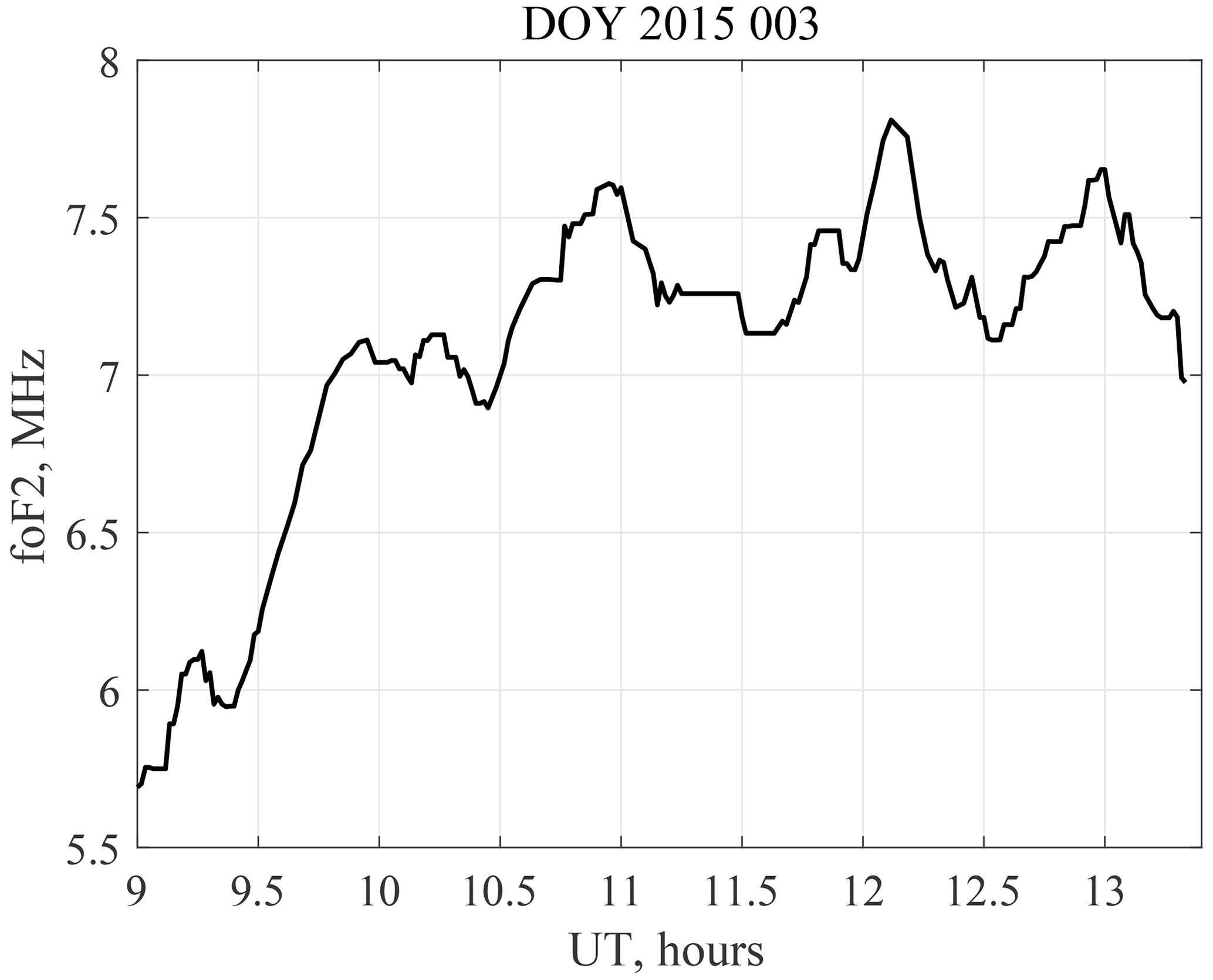
The continuity condition allows us to reduce the effects of multiple reflections and bifurcations. The ASCII files of the retrieved foF2, the approximation parameters, and plots of foF2 time series are available in the Supplement. In all the cases, the results of the automated procedure were tested visually for each tenth data point. The selected intervals form the database for the analysis. As an example, Fig. 2 shows a time variation of the foF2 critical frequency for 3 January 2015 retrieved by the automated procedure.
2.3 Pre-processing, statistical and spectral analysis
We have analyzed pulsations in the meridional component of the geomagnetic field in association with variations of foF2 critical frequency. In the present study we consider geomagnetic pulsations in the 1–5 mHz frequency band with no division into classes Pc5, Pc6 or Pi3. Such a division is often vague, and an automated identification is hardly possible in practice. Moreover, morphological types of pulsations, especially with large azimuthal wave numbers, are not identical in the magnetosphere and on the ground (e.g., Vaivads et al., 2001). Besides, an analysis of the numerous Pc5–6/Pi3 subclasses according to Saito (1978) would be too cumbrous. Thus, we study the inter-relations between all geomagnetic and foF2 variations in the frequency range of the Pc5–6/Pi3 pulsations and investigate their dependencies on the space weather parameters.
One-minute time resolution of the foF2 data allows for the cross-spectral analysis of the Pc5–6/Pi3 geomagnetic pulsations. For these datasets, power spectral density (PSD) and cross-spectral parameters were estimated using the Blackman–Tukey method (Kay, 1988). The cross-spectra have been calculated between the foF2 variations, on the one hand, and geomagnetic pulsations, on the other hand. For the intervals with high spectral coherence, γ2, a phase difference Δφ was estimated. Spectra were calculated for 64 min (Np=64 points) intervals with a 5 min shift. Such a time step allows us to detect short-lived Pi-type pulsations, and an equal length of the time intervals allows us to classify the intervals according to the parameters of their spectra (such as maxima of PSD or coherence or frequency of the PSD maximum) and to use them for statistical analysis. The parameters of spectral analysis are selected as a compromise between the frequency resolution and the dispersion of the spectral estimates. We used a 16-point () window. The dispersion of smoothed coherence spectra can be calculated as
where , and c is a constant depending on the spectral window. Equation (2) shows that the dispersion of coherence depends on its absolute value (Jenkins and Watts, 1969). It goes to zero for high coherence, and it is about the dispersion of non-smoothed spectra for low coherence values. We used as a threshold value of coherence in the present study, which corresponds to a dispersion of 0.074. This means that for , γ2 exceeds 0.25 at 70 % confidence level.
For further analysis, all the intervals were divided into five groups:
-
all intervals in April 2014–December 2015 when space weather parameters and geomagnetic activity indices are analyzed (all intervals, group 1);
-
the intervals, for which spectra of geomagnetic field variations are calculated (Pc5–6/Pi3 intervals, group 2);
-
the intervals, for which spectra of foF2 variations can be calculated (ΔfoF2 intervals, group 3);
-
the intervals in which the coherence of foF2 variations with geomagnetic pulsations exceeded certain threshold (coherent ΔfoF2-bX intervals, group 4);
-
coherent pulsations with a coherence maximum at the high-frequency flank of the band (fγ>2.7 mHz, group 5).
The space weather parameters, activity indices and geomagnetic data are available for most of the intervals. To avoid possible influence of seasonal and diurnal variations, we used data from the same time, 08:00–14:00 UT, when foF2 data were available for the whole year. The total number of intervals in group 3 is 2764. For group 4, it is 448. Note that the pulsations are not independent as some intervals are overlapping, and the numbers of nonoverlapping intervals are 240 and 114 for groups 3 and 4, respectively.
3.1 foF2 variations and geomagnetic pulsations at SOD
3.1.1 Examples
Below we present two examples of the foF2 frequency and geomagnetic field variations simultaneously recorded at SOD. They are characterized by a high ΔfoF2-bX coherence; however, the amplitudes of geomagnetic pulsations were essentially different in these two cases, 4 and 40 nT, respectively. A high-pass filter with cutoff frequency at 0.8 mHz was used for the time series shown in Figs. 3 and 6. To discriminate the deviations of magnetic field and foF2 from their nondisturbed values, the former are denoted as ΔfoF2 and b for foF2 and magnetic field, respectively.
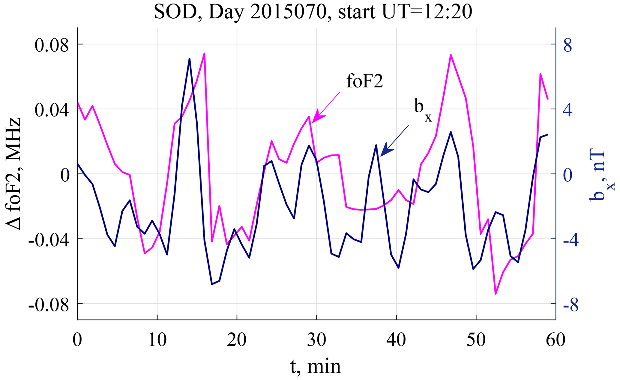
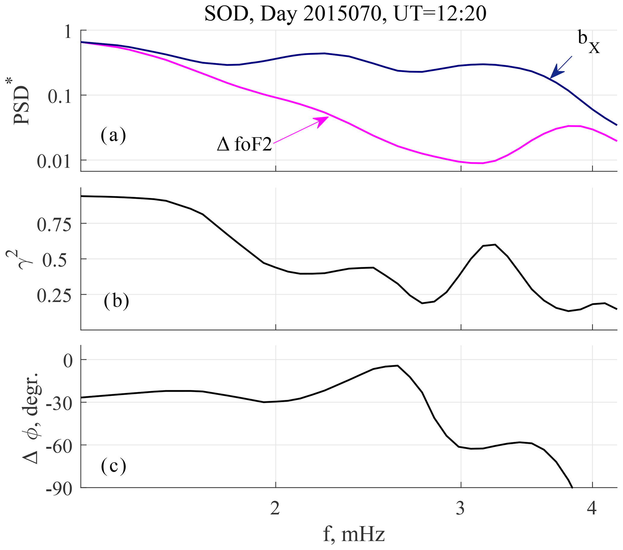
Figure 4Spectral parameters for event 1: (a) normalized PSD spectra of ΔfoF2 and bX pulsations; (b) spectral coherence; and (c) phase difference.
Geomagnetic and foF2 pulsations recorded on 11 March (day 70) 2015 (event 1) are presented in Fig. 3. Peak-to-peak amplitudes of the geomagnetic pulsations and foF2 variations are about 8 nT and 0.05 mHz, respectively. Their maximal values are 12 nT and 0.1 mHz, respectively. The normalized PSD spectra, PSD*, for both geomagnetic and foF2 pulsations, spectral coherence γ2, and phase difference Δφ values are presented in Fig. 4. PSD* of geomagnetic pulsations has two broad maxima at f1=2.3 and f2=3.2 mHz. The spectrum of foF2 variations has a maximum at a frequency f=3.8 mHz. Spectral coherence (γ2>0.75) in the low-frequency part of the spectrum f<2 mHz and a minor coherence peak with γ2=0.6 near the f2 frequency are seen. At f<1.6 mHz where γ2>0.9, the γ2 dispersion does not exceed ; i.e., γ2>0.8 at 83 % confidence level. For γ2=0.75 and 0.6, the dispersion values are 0.027 and 0.056, respectively. Figure 5 shows the space weather conditions for event 1. Zero time in panels (a–e) corresponds to the start time of the interval (12:20 UT). It can be seen that geomagnetic conditions were quiet. Dst nT (Fig. 5a) indicates that no geomagnetic storm occurred for at least 4 d before the event. However, the auroral activity was essential and maximal AE reached 500 nT (Fig. 5b). This activation occurred after a negative (southward) BZ variation of about 20 nT (Fig. 5d). For this event, SW speed V was about 400 km/s (Fig. 5c), and the SW dynamic pressure was about 4 nPa (Fig. 5e). The PSW fluctuations are shown in more detail in Fig. 5f. Their peak-to-peak amplitude was about 0.7 nPa, and their apparent period was about 5 min. This corresponds to a frequency f=3.3 mHz; i.e., it approximately agrees with the f2 frequency of pulsations at SOD.
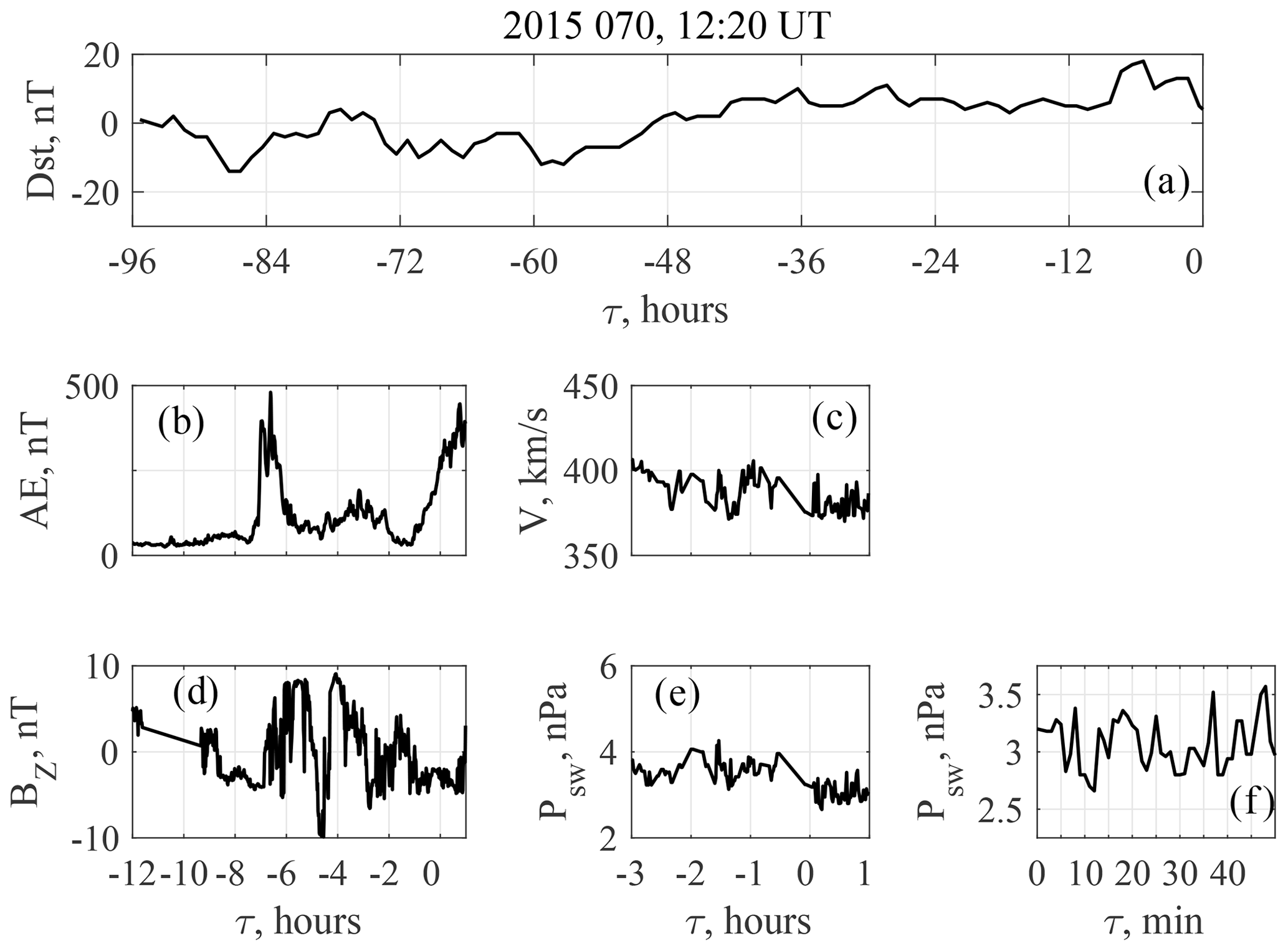
Figure 5Space weather conditions for event 1. (a) Dst index during last 4 d; (b) AE index during the interval and 12 h before; (c) SW speed during the interval and 3 h before; (d) IMF BZ during the interval and 12 h before; (e) SW dynamic pressure during the interval and 3 h before; (f) details of SW dynamic pressure fluctuations during the interval.
The case on 11 July (day 192) 2015 (event 2) is presented in Figs. 6 and 7, which have the same format as Figs. 3 and 4 for the first event. Peak-to-peak amplitudes of geomagnetic and foF2 pulsations are about 80 nT and 0.08 mHz, respectively. A clear maximum at f1≈2.5 mHz is seen in both geomagnetic and ΔfoF2 PSD* spectra (Fig. 7a). At the second frequency f2≈3.5 mHz, a maximum is seen only in the ΔfoF2 PSD* spectrum, while in the bX one this frequency is marked only as a plateau. However, both spectral maxima are clearly visible in the coherence spectrum (Fig. 7b), and the phase difference is different for these two frequencies (Fig. 7c).
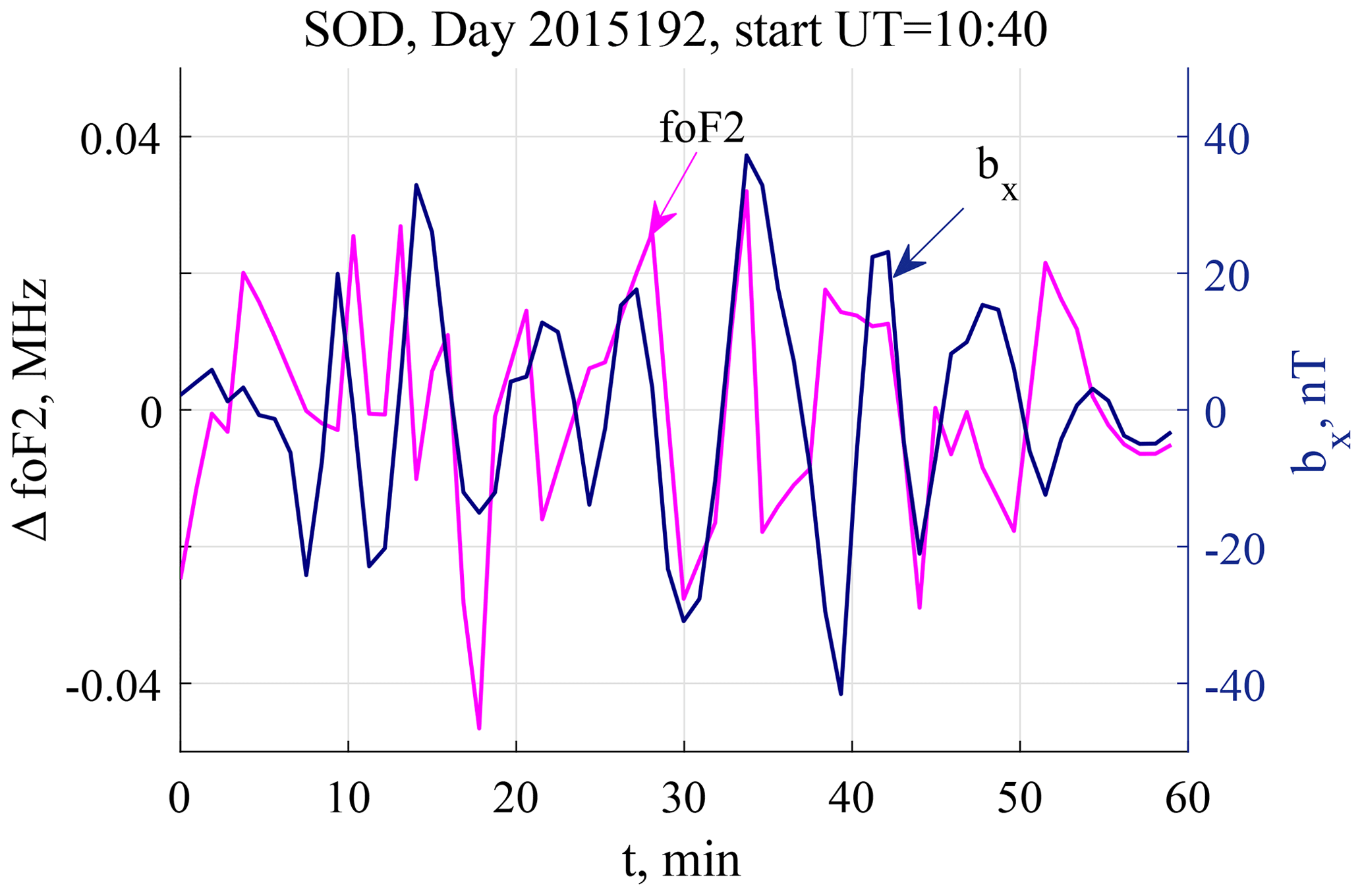
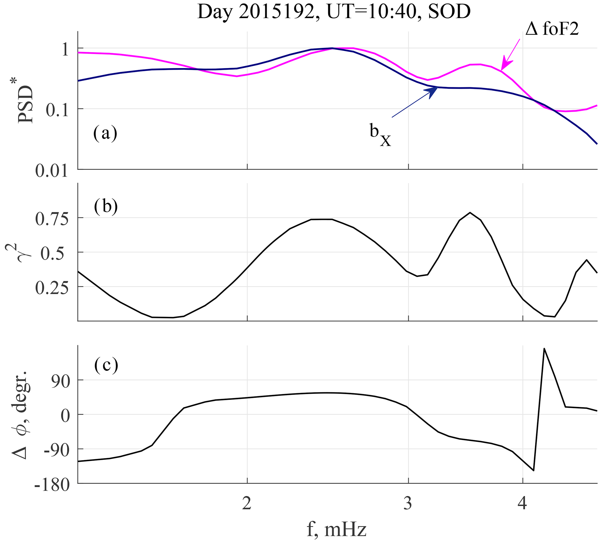
Figure 7Spectral parameters for event 2: (a) normalized PSD spectra of ΔfoF2 and bX pulsations; (b) spectral coherence; and (c) phase difference.
The space weather conditions for this event are summarized in Fig. 8, which has the same format as Fig. 5. There was no geomagnetic storm for 4 d before this event, which is indicated by the Dst exceeding −30 nT (Fig. 8a). Meanwhile, the auroral activity was high, namely, two auroral activations occurred at and −4 h with maximal AE =1300 nT and 700 nT, respectively (Fig. 8b). The first activation occurred after a 2 h interval of negative IMF BZ, while the second one was associated with a BZ turn from −10 nT to almost +15 nT (Fig. 8d). For this event, V was about 600 km/s (Fig. 8c), whereas a maximal PSW was about 9 nPa; then it dropped to 5 nPa and slowly decreased to about 3 nPa (Fig. 8e). The peak-to-peak amplitude of PSW fluctuations during the interval shown in Fig. 8f was about 0.35 nPa. Two types of variations could be observed, namely, fluctuations with an apparent period about 4.5 min and a series of steps at a periodicity of about 7 min. This corresponds to frequencies 3.7 and 2.4 mHz, i.e., near the frequencies of foF2 variations, registered at SOD.
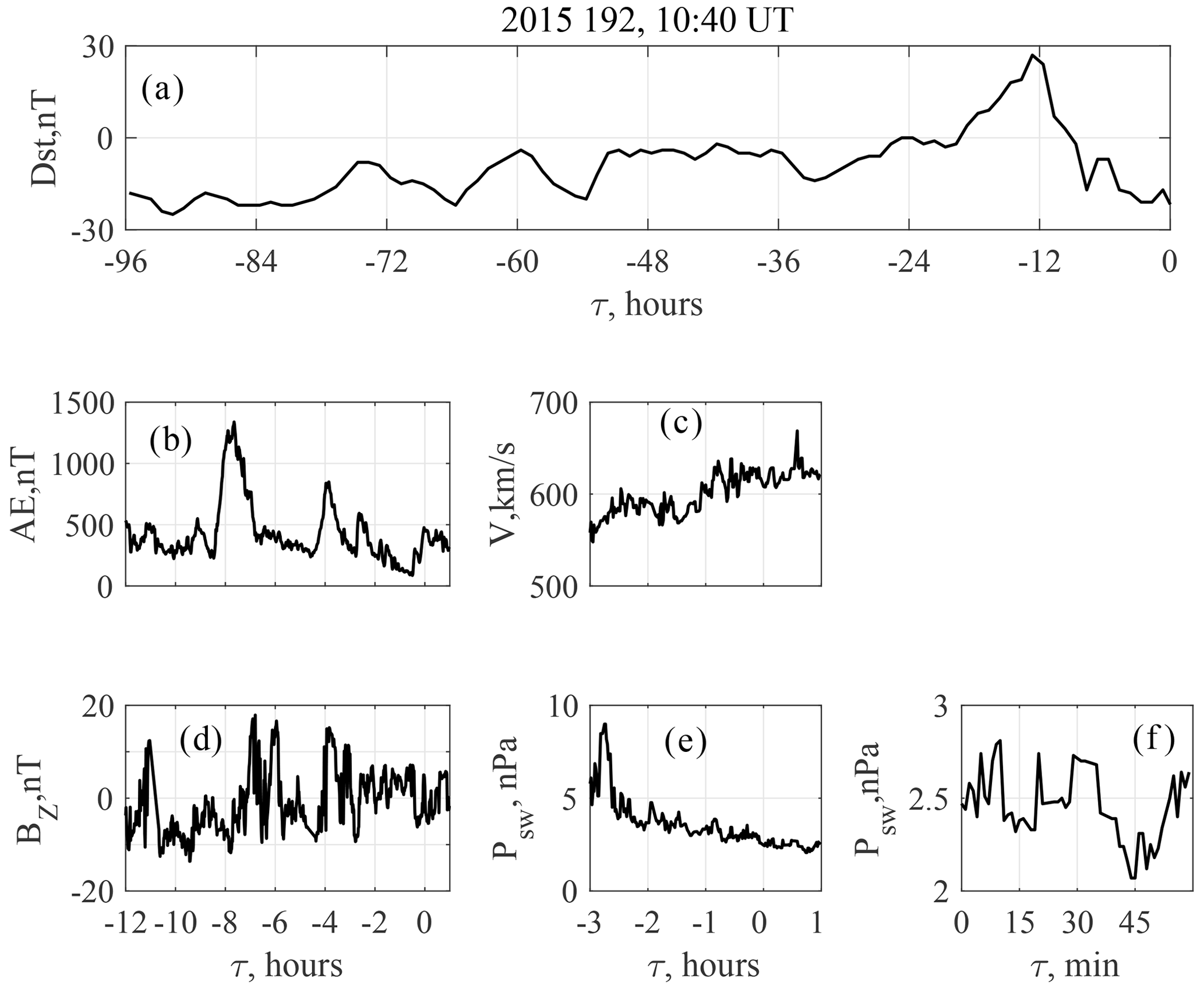
Figure 8Space weather conditions for event 2. (a) Dst index during last 4 d; (b) AE index during the interval and 12 h before; (c) SW speed during the interval and 3 h before; (d) IMF BZ during the interval and 12 h before; (e) SW dynamic pressure during the interval and 3 h before; (f) details of SW dynamic pressure fluctuations.
3.1.2 Statistics
Figure 9 shows the MLT dependence of the ΔfoF2 intervals (group 3) and relative occurrence of coherent events (group 4). One can see from this figure that the foF2 variations were detected in the near-noon and afternoon MLT sectors with a maximal probability between 13:00 and 16:00 MLT. The lower panel shows the relative occurrence of group 4 events. It varies in the range 0.13–0.21 with a maximum near noon.
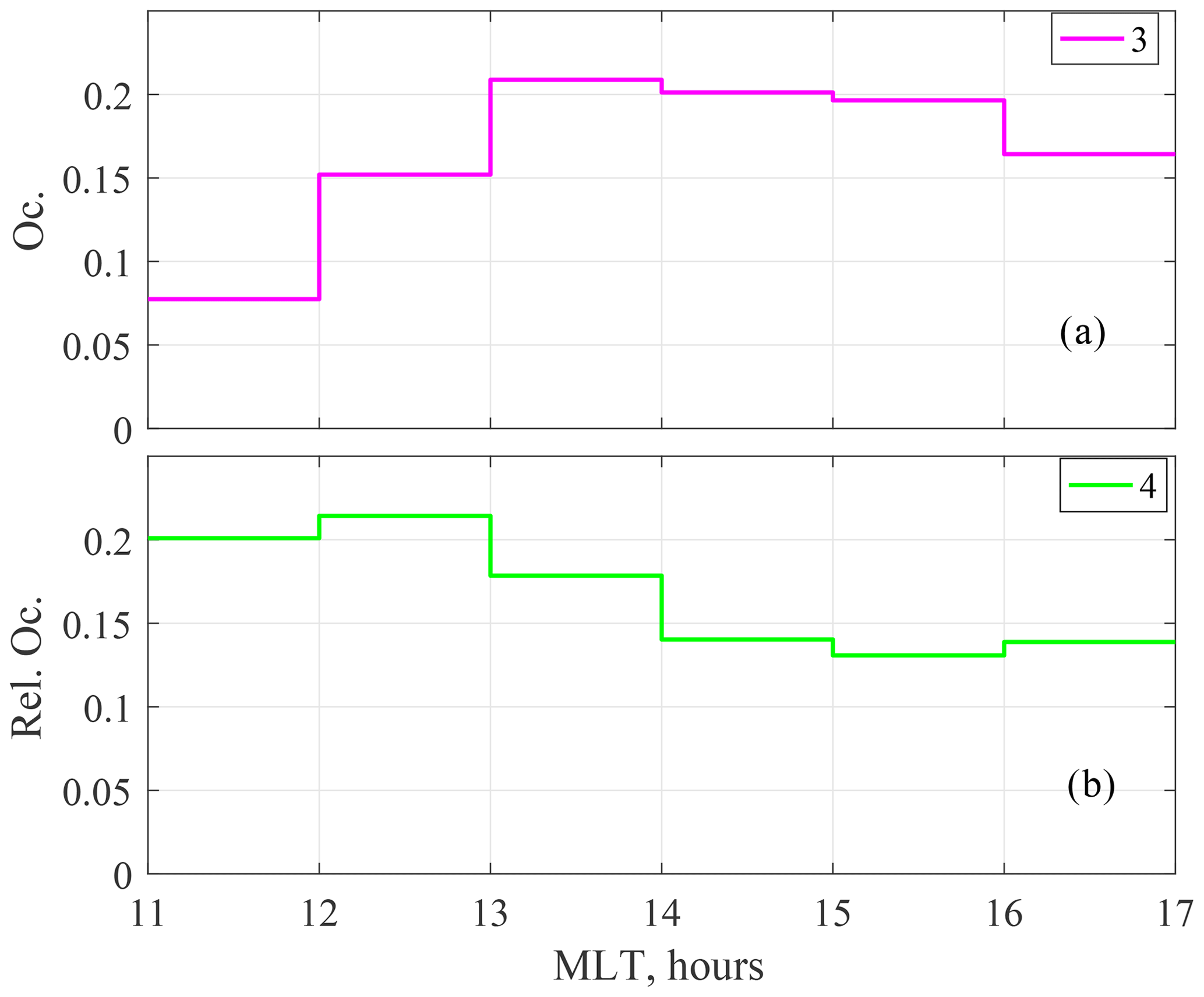
Figure 9(a) The average MLT distribution of occurrence of ΔfoF2 intervals (group 3); (b) relative occurrence of coherent ΔfoF2-bX pulsations (group 4).
Figure 10a shows histograms for the frequencies of local PSD maxima in bX and ΔfoF2 spectra (groups 2 and 3, respectively). The geomagnetic pulsations demonstrate a maximum at 3.2 mHz, which corresponds to the frequency of the Alfvén resonance at the L-shell of SOD. The frequency distribution of ΔfoF2 has two maxima in the frequency bands centered at 2 and 3.9 mHz. Thus, the figure has shown that the most probable frequencies of spectral maxima are different for foF2 and geomagnetic pulsations at SOD.
However, case studies demonstrate that there are pulsations with maxima at the same frequencies in spectra of both ΔfoF2 and bX. To check whether this effect is a random co-incidence or the pulsations are interrelated, we have compared frequency distributions of the foF2 and geomagnetic pulsations for random (not equal, in a general case) time intervals with those recorded simultaneously. We have calculated a square difference, , where fF2 and fb are the frequencies of ΔfoF2 and bX PSD maxima, respectively. The parameter Δf2 was calculated for fF2 and fb taken from the spectra, estimated at random and simultaneous time intervals. To reduce possible influence of diurnal variation, for each fF2 we only used the Δf2 values obtained from bX spectra calculated on a random day at the same MLT with an 1 h accuracy. Then, its average value was calculated. The difference in average values of Δf2 for simultaneous and random intervals was quantified as a parameter , where Δf2,0 and Δf2,R are the mean values of Δf2 for simultaneous and random intervals, respectively. Negative values of δ indicate that the frequencies agree better for simultaneous than for random intervals. The frequency dependence of δ is shown in Fig. 10b. One can see that δ is negative in all the frequency bands, except one centered at 2.5 mHz. A minimum is observed at f=3.2 mHz, i.e., near the Alfvén resonant frequency at SOD. Mostly negative values of δ indicate that the frequencies of geomagnetic and foF2 pulsations are closer to each other for the simultaneous time intervals than for the random ones. Therefore, there has to be a process responsible for synchronization of the geomagnetic and foF2 pulsations.
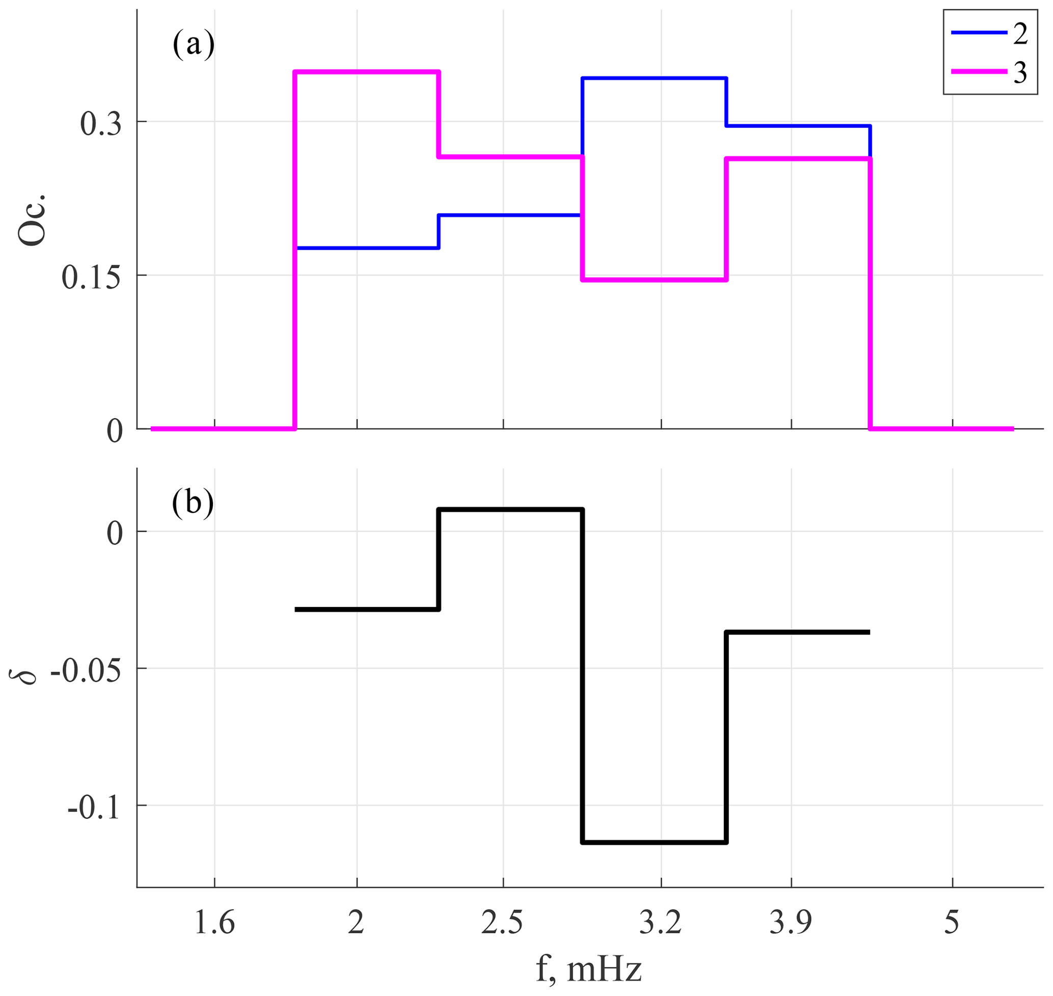
Figure 10Frequency histogram for bX (group 2) and ΔfoF2 (group 3) fluctuations (a) and for the parameter , where Δf2,0 and Δf2,R are the mean values of Δf2 for simultaneous and random intervals, respectively (b).
The inter-relation between geomagnetic and foF2 pulsations is manifested also in the coherent ΔfoF2-bX pulsations. Then a question arises. How does the probability to detect a coherent ΔfoF2-bX pulsation depend on the parameters of geomagnetic pulsation and the space weather? To answer this question, we have studied three groups of parameters:
-
PSD, polarization and spatial distribution of geomagnetic pulsations;
-
indices of geomagnetic storms (Dst) and auroral (AE) activity; and
-
the interplanetary parameters controlling geomagnetic activity.
First, we compared the parameters of geomagnetic pulsations at SOD for the Pc5–6/Pi3 intervals (group 2), ΔfoF2 intervals (group 3) and coherent ΔfoF2-bX intervals (group 4).
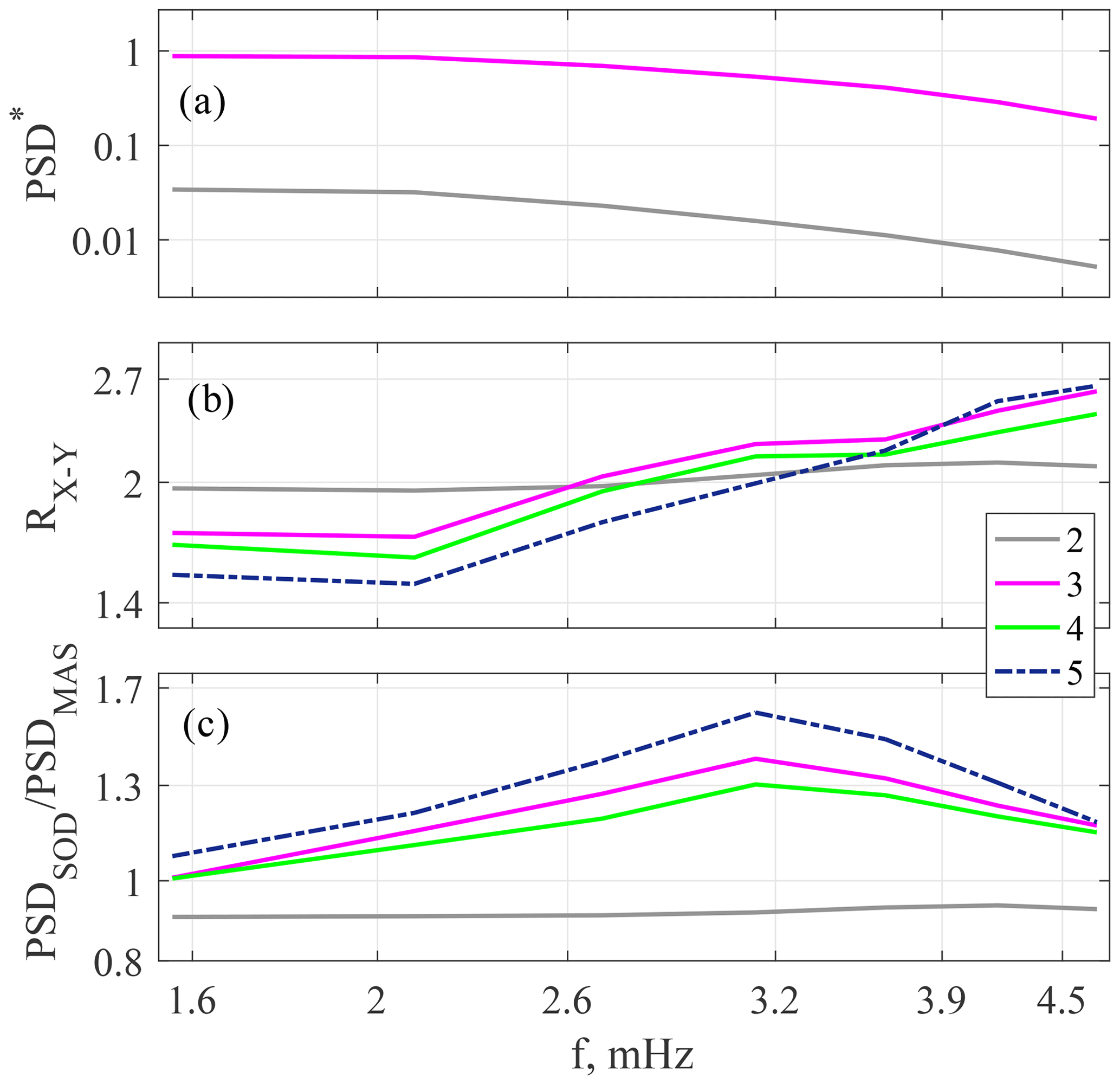
Figure 11Comparison of Pc5-3/Pi3 parameters for Pc5-3/Pi3 (group 2), ΔfoF2 (group 3), coherent ΔfoF2-bX (group 4) and high-frequency coherent ΔfoF2-bX (group 5) intervals: (a) PSD; (b) ; (c) meridional PSD ratio .
The results are presented in Fig. 11. The PSDs of geomagnetic pulsations are shown at panel 11a for groups 2 and 3. The results for group 4 are almost the same as those for group 3 (not shown here). The PSD in group 3 is higher than that in group 2 at all frequencies. We think this is due to the selection criteria for the ΔfoF2 intervals.
Polarization of the pulsations has been analyzed with a PSD ratio , and the result is shown in Fig. 11b. To test the hypothesis about possible influence of the Alfvén field line resonance (FLR) on the ΔfoF2-bX interrelation, group of coherent pulsations with a high-frequency coherence maximum (group 5) is included in the analysis. The difference between group 2 and all the ΔfoF2 groups (3–5) is indicated by a growth of RXY for the latter at f>2 mHz. The slope of RXY is maximal for group 5.
Following Baransky et al. (1995), we have used a meridional PSD ratio in the resonance bX component calculated with the SOD–MAS station pair PSDSOD/PSDMAS. In contrast to group 2, meridional PSD ratios for groups 3–5 have maxima at f=3.2 mHz. The curves for groups 3 and 4 are very similar, and the effect is maximal for group 5.
Thus, geomagnetic pulsations, recorded during ΔfoF2 intervals, are polarized mostly along the meridian at the high-frequency flank of the spectrum. They also demonstrate a maximum in meridional PSD ratio at f=3.2 mHz, i.e., near the Alfvén resonant frequency at SOD.

The distribution of pulsations for groups 2–4 over the maximal PSD of bX, PSDmax, is given in Fig. 12. The upper panel shows the distribution for groups 2 and 3. The most probable PSDmax values are nT2/Hz for group 2, whereas for group 3 they are nT2/Hz, i.e., 3 times higher. The relative occurrence of group 4 weakly depends on bX PSD. It has a maximum in the same PSD band, in which the probability maximum is found. This value of PSD is common enough, and the pulsations in this PSD band were observed in approximately 20 % of the spectra.
Statistics on ΔfoF2 and bX fluctuations related to different levels of geomagnetic activity are presented in Fig. 13. Left panels (13a, c) present the occurrence distribution for all ΔfoF2 and coherent ΔfoF2-bX intervals (groups 1, 3 and 4). Right panels (13b, d) demonstrate group 4 relative occurrence.
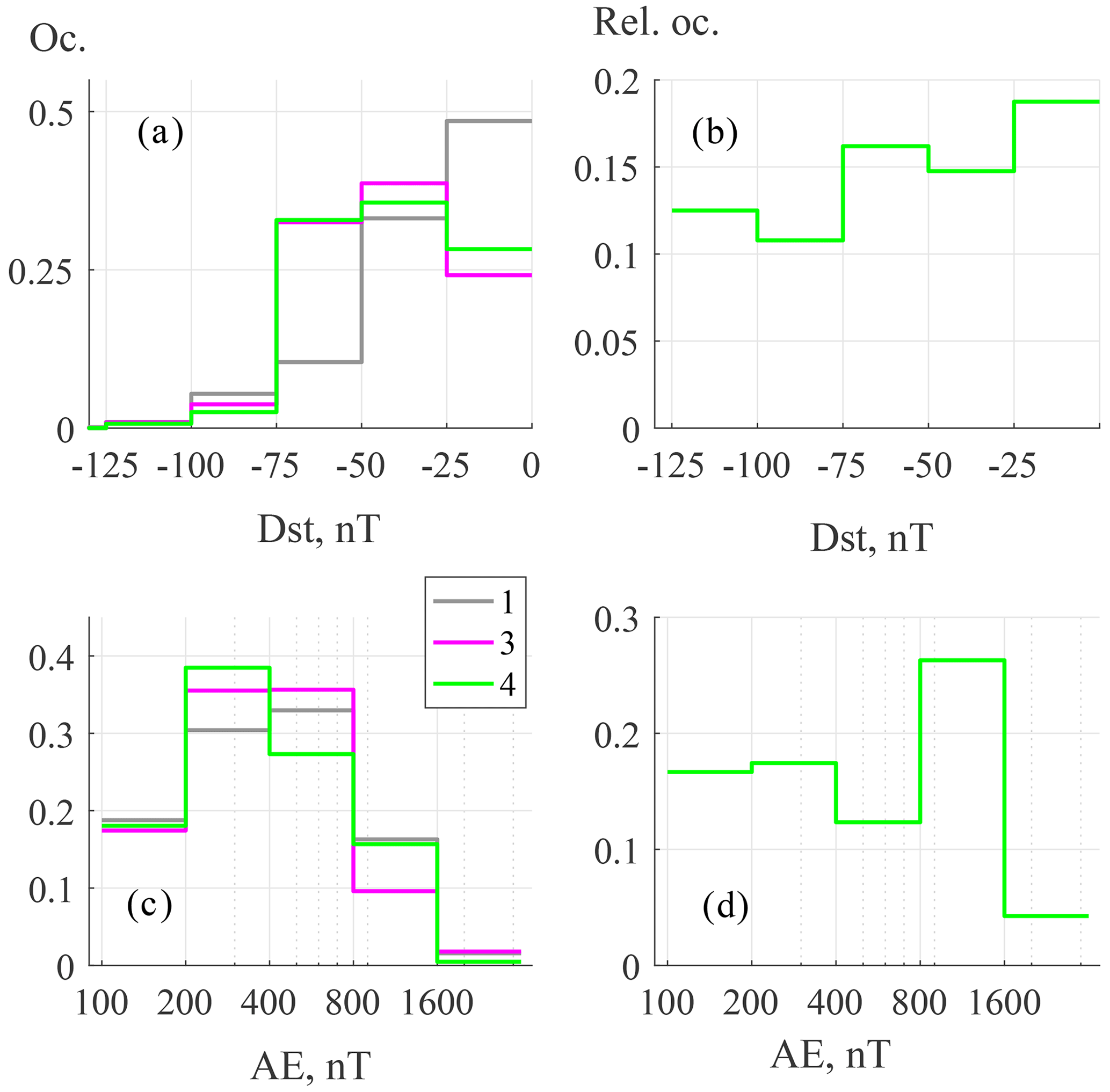
Figure 13Left panels show activity index distributions for groups 1, 3 and 4: Dst (a) and AE (c). Right panels show the same for group 4 relative occurrence: Dst (b) and AE (d).
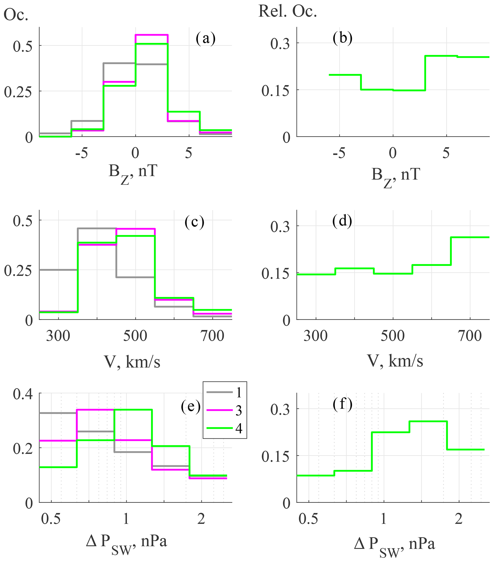
Figure 14Left panels show SW/IMF parameter distributions for groups 1, 3 and 4: IMF BZ (a), V (c) and ΔPSW (e). Right panels show the same for group 4 relative occurrence: BZ (b), V (d) and ΔPSW (f).
An interval is defined as a post-storm one if the 4 d minimal Dst drops below −25 nT. Geomagnetic and foF2 pulsations in such cases start within several hours after the Dst minimum, i.e., at the main phase of the magnetic storm, or at the recovery phase, i.e., when time delay τ exceeds 12 h. The probability maximum for groups 3 and 4 is found for the Dst range nT, which corresponds to a weak geomagnetic storm. For both groups, the occurrence at Dst nT exceeds that for the background group (group 1). At this Dst level, more than 70 % of the pulsations were observed at the recovery phase of a storm. The maximal occurrence was found at τ≈2 d. Time delay distributions for different storm intensities are available in Fig. S1 in the Supplement. Relative occurrence of coherent ΔfoF2-bX intervals (group 4) is somewhat higher for moderate and low storm activity: Dst nT compared to Dst nT (Fig. 13b).
The most important difference in the AE distributions of groups 1 and 3 was found for the AE values between 800 and 1600 nT (Fig. 13c). For this AE interval, the occurrence for group 3 is 0.1 against 0.17 for group 1. This is compensated by enhanced probability of AE in the range (200–800) nT for group 3 compared to group 1. The group 4 occurrence at AE within (800–1600) nT is about the same as for group 1. This is also emphasized in the enhanced group 4 relative occurrence (0.26) for this level of AE against 0.17 at AE <400 nT (Fig. 13d).
Summarizing, we can say that intervals after moderate magnetic storms are favorable for foF2 fluctuations in the Pc5–6/Pi3 range. However, no essential difference in Dst was found between groups 3 and 4. Fluctuations of foF2 were registered predominantly under a moderate auroral activity. Meanwhile, higher levels of auroral activity, namely, (800–1600) nT AE, are favorable for coherent ΔfoF2-bX pulsations.
The statistical results for interplanetary parameters are presented in Fig. 14. The IMF BZ controls the energy input from the solar wind to the magnetosphere. Generally, all auroral phenomena, including Pc5–6/Pi3 pulsations, are more intensive and occur at lower latitudes during negative IMF BZ. A positive IMF BZ causes enhanced activity at higher latitudes. The IMF BZ distributions for groups 1, 3 and 4 (all, ΔfoF2 and coherent ΔfoF2-bX intervals) are shown in Fig. 14a and b. While the distribution for group 1 is almost symmetrical, groups 3 and 4 are both shifted to positive BZ values. This effect is stronger for group 4. The group 4 relative occurrence was maximal at nT (Fig. 14b). The results for the SW speed are given in Fig. 14c and d. The main difference between groups 1 and 3/4 was found in the bands centered at 500 and 300 km/s. The distributions for the latter groups are shifted to higher SW speeds. This might be due to an artifact of the initial selection procedure, which sets a lower boundary for the amplitude of geomagnetic pulsations. An important difference between groups 3 and 4 can be seen in Fig. 14d, which demonstrates a maximal group 4 relative occurrence at high SW speed, namely, in the band centered at 700 km/s.
The results for amplitudes of the SW dynamic pressure fluctuations are given at bottom panels (Fig. 14e, f). The most probable amplitude is higher for group 4 than for group 3 and for group 3 than for group 1. This effect is also seen for group 4 for which relative occurrence reached 0.27 in the ΔPSW range (1.3–1.8) nPa against 0.13 at ΔPSW<0.9 nPa.
To summarize, the foF2 fluctuations were preferably recorded under positive IMF BZ, moderate V≈500 km/s SW speed and amplitudes of PSW fluctuations within (0.6–0.9) nPa.
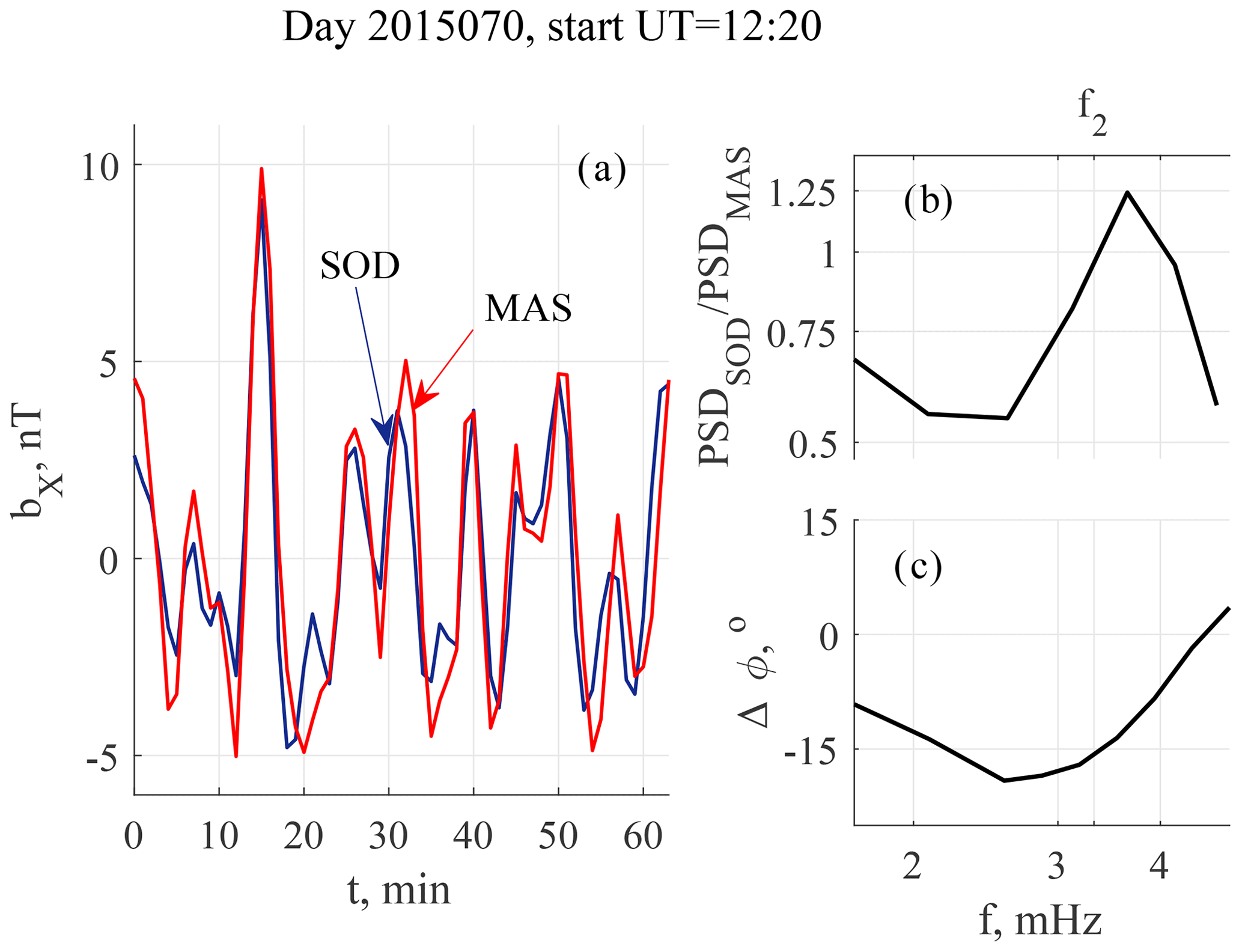
Figure 15Illustration of FLR signatures of geomagnetic pulsations on 11 March (event 1). Pulsation waveforms at SOD and MAS (a); meridional PSD ratio (b) and phase difference (c).
The present study of daytime fluctuations of foF2 in the 1–5 mHz frequency range has been undertaken for quiet and moderately disturbed geomagnetic conditions when the foF2 frequency can be unambiguously retrieved from ionograms. For that, a technique of automated scaling of foF2 was developed and verified by visual inspection.
Our results show a weak inter-relation between geomagnetic Pc5–6/Pi3 pulsations and foF2 variations in the same frequency range. The coherent ΔfoF2-bX pulsations can occur at typical Pc5–6/Pi3 amplitudes. The most probable PSD band for these types of pulsations is recorded as often as at each fifth interval. In these cases, the characteristics of magnetic pulsations such as the spectral content, polarization and meridional PSD ratio allow us to interpret them as the Alfvén FLR following Baransky et al. (1995).
The Alfvén FLR features can also be seen in the spatial structure of Pc5 pulsations in events 1 and 2, which are discussed in Sect. 3.1.1. The Pc5 records at SOD and MAS for event 1 are shown in Fig. 15 along with meridional PSD ratio and phase difference. Waveforms of the pulsations are very similar; however, the phase is slightly delayed at MAS. The meridional PSD ratio is below 1 at the low-frequency flank of the spectrum, and it is growing at f>2.7 mHz, reaching a maximum at 3.7 mHz (Fig. 15b). The f2 frequency of the second ΔfoF2-bX coherence maximum is near the frequency of maximal growth of meridional PSD ratio. A phase difference in this frequency band is about (Fig. 15c).
A similar result was obtained in the comprehensive statistical analysis of the correspondence between geomagnetic pulsations and pulsations in the Cosmic Noise Absorption (CNA) by Spanswick et al. (2005), who found that geomagnetic pulsations with FLR features demonstrate a better correspondence with CNA pulsations than non-FLR Pc5s. However, physical reasons for our results and those of Spanswick et al. (2005) may be different, due to different energies of precipitating particles and types of geomagnetic pulsations. A detailed case study of pulsations in the magnetic field and the electron flux at four Cluster satellites located at different L-shells in the magnetosphere and geomagnetic and CNA pulsations on the ground (Motoba et al., 2013) showed rather complicated space distributions and time variations of geomagnetic and electron flux pulsations and their inter-relations. The pulsation in space was, probably, a mix of compressional and shear Alfvén modes. The authors found that the amplitude of compressional mode was critical for effective modulation of electron flux, but the contribution of shear Alfvén resonance was also non-negligible.
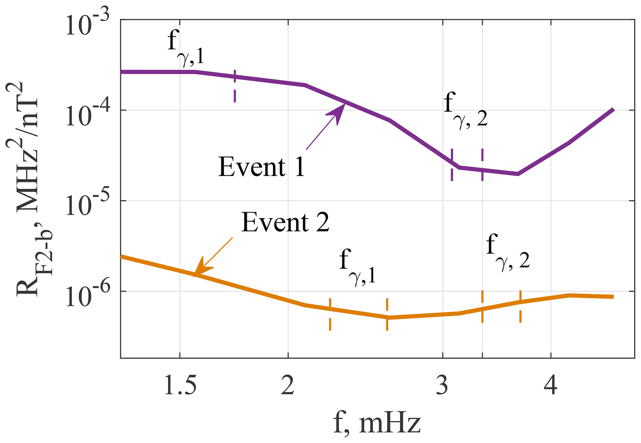
Figure 16Comparison of ΔfoF2 to bX PSD ratios RF2−b for events 1 and 2. The bands of high ΔfoF2-bX coherence are shown with vertical dashed lines.
The foF2 was automatically retrieved from ionograms preferably near noon and in the afternoon under moderately disturbed geomagnetic conditions. As a rule, the afternoon Pc5 waves are characterized by higher azimuthal wave numbers than morning-side Pc5s (see Min et al., 2017, and references therein). They are often associated with kinetic modes originated from the wave–particle interactions (see e.g., Mager et al., 2013, and references therein). For these waves, the amplitudes on the ground are strongly attenuated by the ionosphere (Kokubun et al., 1989), while their amplitudes in the magnetosphere both in the magnetic field and in particle flux can be high (Baddeley et al., 2004). High-m waves generated by unstable ion distributions can effectively interact with ULF waves in the Pc4 range (Baddeley et al., 2005). A comprehensive analysis of ion distribution functions in the magnetosphere undertaken by Baddeley et al. (2005) proved that the free energy of ion population provided observed magnitudes of high-m ULF waves in the ionosphere.
These pulsations typically occur during auroral activations. Auroral substorms are followed by Pi3 pulsations (Kleimenova et al., 2002) and Pc5 waves with high and intermediate azimuthal wavenumbers (Zolotukhina et al., 2008; Mager et al., 2019). A substorm can generate magnetospheric waves with a wide spectrum of azimuthal wave numbers (James et al., 2016). The large-scale waves are detected on Earth, whereas the small-scale waves modulate particle flux and are manifested in electron precipitation into the ionosphere. In such a situation, no strong dependence can be expected between the amplitudes of pulsations of the ionospheric electron density and geomagnetic field on Earth.
Geomagnetic pulsations recorded simultaneously in the magnetosphere and on Earth were studied by Watson et al. (2015). Their study clearly demonstrated that ULF waves effectively modulated electron flux at geostationary orbit and TEC in the ionosphere. Probably, a flux of soft electrons was modulated by the wave. This allowed us to explain the observed values of TEC modulation. Different contributions of shear Alfvén and compressional modes to the ULF power in the magnetosphere results in different values of TEC to magnetic field amplitude ratio on the ground. This can explain the contrast in TEC to geomagnetic pulsation amplitude ratio found by Watson et al. (2015) and Pilipenko et al. (2014a) and between the two example events in the present study.
The ΔfoF2 to bX PSD ratio, RF2−b, is essentially higher for event 1 than for event 2. Figure 16 shows a frequency dependence of RF2−b for these two events. The maximal difference is seen at about 2 mHz, and it is more than 2 orders of magnitude (more than an order of magnitude in the amplitude ratio). At frequencies of the second coherence maxima, the difference is more than an order of magnitude. The main visible difference between geomagnetic pulsations for these two events can be seen in their waveforms. The foF2 and geomagnetic field variations during event 1 have a well-correlated long-period part at f<1.6 mHz. This may be a result of some global process, which is responsible for both geomagnetic pulsations and particle modulation. Fluctuations of SW dynamic pressure are one of the sources of global geomagnetic pulsations inside the magnetosphere (Kepko et al., 2002; Yagova et al., 2007; Viall et al., 2009). Indeed, the coherent ΔfoF2-bX pulsations are preferably associated with fluctuating PSW, and periods of the foF2 fluctuations are often close to those of PSW. However, in the present study we can not judge whether or not the ULF waves are global. To test this hypothesis, a separate study would be needed.
We suggested a technique for the automated detection of foF2, which allows us to obtain data suitable for spectral estimates and comparison with Pc5–6/Pi3 geomagnetic pulsations. The foF2 variations show some inter-relation with Pc5–6/Pi3 geomagnetic pulsations, not only for extremely high but also for typical values of PSD, as well. Geomagnetic pulsations for which ΔfoF2-bX coherence is higher at f>2.7 mHz demonstrate the Alfvén FLR features.
Variations of the ionospheric critical frequency foF2 were observed predominantly at noon and in the afternoon under quiet or moderately disturbed geomagnetic conditions, namely, at the recovery phase of a weak or moderate geomagnetic storm and moderate auroral activity (6 h maximal AE <800 nT). Meanwhile, the interplanetary parameters were positive (northward) IMF BZ, moderate SW speed (V≃500 km/s) and amplitudes of SW dynamic pressure fluctuations of about 0.7 nPa.
The coherent ΔfoF2-bX pulsations tend to occur during an enhanced auroral activity (AE >800 nT). Compared to the non-coherent cases, they preferably occur under higher values of positive IMF BZ, higher SW velocity and larger amplitudes of SW dynamic pressure fluctuations.
Code used in the paper is available at https://www.sgo.fi/pub/AnnGeo_2021_39_1/CODES/ (last access: 11 June 2021, nyagova@ifz.ru) (Yagova et al., 2021).
Data used in the paper are available at https://www.sgo.fi/pub/AnnGeo_2021_39_1/DATA/ (last access: 11 June 2021, alexander.kozlovsky@oulu.fi) (Yagova et al., 2021).
The foF2 values, obtained with Eq. (1) for all the intervals analyzed, are available both as JPEG images and ASCII files. A file name has a structure SOD-YYYY-DDD-foF2, where YYYY is a year and DDD is a day number. Each ASCII file contains two columns:
-
time (seconds) from 00:00 UT,
-
foF2 (mHz).
ASCII files with approximation parameters for Eq. (1) are available, and a description of the columns is in the appr-readme.txt file. The supplement related to this article is available online at: https://doi.org/10.5194/angeo-39-549-2021-supplement.
NY contributed to the approximation algorithm and cross-spectral and statistical analyses. AK contributed to the pre-processing and visual check of ionosonde data. EF contributed to interpretation of results and analysis of wave parameters. OK contributed to selection of events, algorithms and codes for visualization. All the authors contributed to the preparation of the article.
The authors declare that they have no conflict of interest.
We thank SGO (http://www.sgo.fi/, last access: 28 April 2021) for SOD magnetometer and ionosonde data, Finnish Meteorological Institute for MAS magnetometer data, CDAWEB (https://cdaweb.gsfc.nasa.gov, last access: 28 April 2021) for OMNI data and World Data Center for Geomagnetism, Kyoto, (http://wdc.kugi.kyoto-u.ac.jp/index.html, last access: 28 April 2021) for AE and Dst indices. Useful discussions with Vyacheslav Pilipenko are appreciated. The authors thank Sergey Kaverznev for text editing as well as the topical editor and both referees for their helpful remarks.
This research has been supported by the Academy of Finland (grant nos. 298578 and 310348), the Russian Foundation for Basic Research (RFBR) (grant no. 20-05-00787) and the state contract with IPE (NY, EF).
This paper was edited by Georgios Balasis and reviewed by two anonymous referees.
Baddeley, L. J., Yeoman, T. K., Wright, D. M., Trattner, K. J., and Kellet, B. J.: A statistical study of unstable particle populations in the global ringcurrent and their relation to the generation of high m ULF waves, Ann. Geophys., 22, 4229–4241, https://doi.org/10.5194/angeo-22-4229-2004, 2004. a
Baddeley, L. J., Yeoman, T. K., Wright, D. M., Trattner, K. J., and Kellet, B. J.: On the coupling between unstable magnetospheric particle populations and resonant high m ULF wave signatures in the ionosphere, Ann. Geophys., 23, 567–577, https://doi.org/10.5194/angeo-23-567-2005, 2005. a, b, c
Baker, G., Donovan, E. F., and Jackel, B. J.: A comprehensive survey of auroral latitude Pc5 pulsation characteristics, J. Geophys. Res., 108, 1384, https://doi.org/10.1029/2002JA009801, 2003. a
Baransky, L. N., Fedorov, E. N., Kurneva, N. A., Pilipenko, V. A., Green, A. W., and Worthington, E. W.: Gradient and polarization methods of the ground-based hydromagnetic monitoring of magnetospheric plasma, J. Geomagn. Geolect., 47, 1293–1309, 1995. a, b
Bargatze, L. F., McPherron, R. L., Minamora, J., and Weimer, D.: A new interpretation of Weimer et al's solar wind propagation delay technique, J. Geophys. Res., 110, A07105, https://doi.org/10.1029/2004JA010902, 2005. a
Buchert, S. C., Fujii, R., and Glassmeier, K.-H.: Ionospheric conductivity modulation in ULF pulsations, J. Geophys. Res., 104, 10119–10133, https://doi.org/10.1029/1998JA900180, 1999. a
Davies, K. and Hartmann, G. K.: Short-period fluctuations in total columnar electron content, J. Geophys. Res., 81, 3431–3434, https://doi.org/10.1029/JA081i019p03431, 1976. a, b, c
James, T. K., Yeoman, M. K., Mager, P. N., and Klimushkin, D. Y.: Multiradar observations of substorm-driven ULF waves, J. Geophys. Res.-Space Physics, 121, 5213–5232, https://doi.org/10.1002/2015JA022102, 2016. a, b
Jenkins, G. M. and Watts, D. G.: Spectral analysis and its application, Holden day, San Francisco, London Amsterdam, 525 pp., 1969. a
Kay, S. M.: Modern spectral estimation: Theory and application, Prentice-Hall, New Jersey, USA, 543 pp., 1988. a
Kleimenova, N. G., Kozyreva, O. V., Kauristie, K., Manninen, J., and Ranta, A.: Case studies on the dynamics of Pi3 geomagnetic and riometer pulsations during auroral activations, Ann. Geophys., 20, 151–159, https://doi.org/10.5194/angeo-20-151-2002, 2002. a
Kepko, L., Spence, H. E., and Singer, H. J.: ULF waves in the solar wind as direct drivers of magnetospheric pulsations, Geophys. Res. Lett., 29, 1197, https://doi.org/10.1029/2001GL014405, 2002. a
Kokubun, S., Erickson, K. N., Fritz, T. A., and McPherron, R. L.: Local time asymmetry of Pc 4-5 pulsations and associated particle modulations at synchronous orbit, J. Geophys. Res., 94, 6607–6625, https://doi.org/10.1029/JA094iA06p06607, 1989. a
Kozlovsky, A., Turunen, T., and Ulich, T.: Rapid-run ionosonde observations of traveling ionospheric disturbances in the auroral ionosphere, J. Geophys. Res.-Space, 118, 5265–5276, https://doi.org/10.1002/jgra.50474, 2013. a
Kozyreva, O., Kozlovsky, A., Pilipenko, V., and Yagova, N.: Ionospheric and geomagnetic Pc5 oscillations as observed by the ionosonde and magnetometer at Sodankylä, Adv. Space Res., 63, 2052–2065, https://doi.org/10.1016/j.asr.2018.12.004, 2019. a
Mager, O. V., Chelpanov, M. A., Mager, P. N., Klimushkin, D. Y., and Berngardt, O. I.: Conjugate ionosphere-magnetosphere observations of a sub-Alfvénic compressional intermediate-m wave: A case study using EKB radar and Van Allen Probes, J. Geophys. Res.-Space, 124, 3276–3290, https://doi.org/10.1029/2019JA026541, 2019. a, b
Mager, P. N., Klimushkin, D. Yu., and Kostarev, D. V.: Drift-compressional modes generated by inverted plasma distributions in the magnetosphere, J. Geophys. Res.-Space, 118, 4915–4923, https://doi.org/10.1002/jgra.50471, 2013. a
Min, K., Takahashi, K., Ukhorskiy, A. Y., Manweiler, J. W., Spence, H. E., Singer, H. J., Claudepierre, S. G., Larsen, B. A., Soto-Chavez, A. R., and Cohen, R. J.: Second harmonic poloidal waves observed by Van Allen Probes in the dusk-midnight sector, J. Geophys. Res.-Space, 122, 3013–3039, https://doi.org/10.1002/2016JA023770, 2017. a
Motoba, T., Takahashi, K., Gjerloev, J., Ohtani, S., and Milling, D. K.: The role of compressional Pc5 pulsations in modulating precipitation of energetic electrons, J. Geophys. Res.-Space, 118, 7728–7739, https://doi.org/10.1002/2013JA018912, 2013. a
Okuzawa, T. and Davies, K.: Pulsations in total columnar electron content, J. Geophys. Res., 86, 1355–1363, https://doi.org/10.1029/JA086iA03p01355, 1981. a, b, c
Pilipenko, V., Belakhovsky, V., Kozlovsky, A., Fedorov, E., and Kauristie, K.: ULF wave modulation of the ionospheric parameters: Radar and magnetometer observations, J. Atmos. Sol. Terr. Phys., 108, 68–76, https://doi.org/10.1016/j.jastp.2013.12.015, 2014a. a, b, c
Pilipenko, V., Belakhovsky, V., Murr, D., Fedorov, E., and Engebretson, M.: Modulation of total electron content by ULF Pc5 waves, J. Geophys. Res.-Space, 119, 4358–4369, https://doi.org/10.1002/2013JA019594, 2014b. a, b
Ren, J., Zong, Q. G., Zhou, X. Z., Spence, H. E., Funsten, H. O., Wygant, J. R., and Rankin, R.: Cold plasmaspheric electrons affected by ULF waves in the inner magnetosphere: A Van Allen Probes statistical study, J. Geophys. Res., 124, 7854–7965, https://doi.org/10.1029/2019JA027009, 2019. a
Ruohoniemi, J. M., Greenwald, R. A., Baker, K. B., and Samson, J. C.: HF radar observations of Pc 5 field line resonances in the midnight/early morning MLT sector, J. Geophys. Res., 96, 15697–15710, https://doi.org/10.1029/91JA00795, 1991. a
Saito, T.: Long-period irregular magnetic pulsations, Pi3, Space Sci. Rev., 21, 427–467, https://doi.org/10.1007/BF00173068, 1978. a
Spanswick, E., Donovan, E., and Baker, G.: Pc5 modulation of high energy electron precipitation: particle interaction regions and scattering efficiency, Ann. Geophys., 23, 1533–1542, https://doi.org/10.5194/angeo-23-1533-2005, 2005. a, b
Tanskanen, E. I.: A comprehensive high-throughput analysis of substorms observed by IMAGE magnetometer network: Years 1993–2003 examined, J. Geophys. Res., 114, A05204, https://doi.org/10.1029/2008JA013682, 2009. a
Vaivads, A., Baumjohann, W., Georgescu, E., Haerendel, G., Nakamura, R., Lessard, M. R., Eglitis, P., Kistler, L. M., and Ergun, R. E.: Correlation studies of compressional Pc5 pulsations in space and Ps6 pulsations on the ground, J. Geophys. Res., 106, 29797–29806, https://doi.org/10.1029/2001JA900042, 2001. a
Viall, N. M., Kepko, L., and Spence, H. E.: Relative occurrence rates and connection of discrete frequency oscillations in the solar wind density and dayside magnetosphere, J. Geophys. Res., 114, A01201, https://doi.org/10.1029/2008JA013334, 2009. a
Vorontsova, E., Pilipenko, V., Fedorov, E., Sinha, A. K., and Vichare, G.: Modulation of total electron content by global Pc5 waves at low latitudes, Adv. Space Res., 57, 309–319, https://doi.org/10.1016/j.asr.2015.10.041, 2016. a
Watson, C., Jayachandran, P. T., Singer, H. J., Redmon, R. J., and Danskin, D.: Large-amplitude GPS TEC variations associated with Pc5–6 magnetic field variations observed on the ground and at geosynchronous orbit, J. Geophys. Res.-Space, 120, 7798–7821, https://doi.org/10.1002/2015JA021517, 2015. a, b, c, d
Wright, D. M., Yeoman, T. K., and Chapman, P. J.: High-latitude HF Doppler observations of ULF waves. 1. Waves with large spatial scale sizes, Ann. Geophys., 15, 1548–1556, https://doi.org/10.1007/s00585-997-1548-2, 1997. a
Yagova, N., Pilipenko, V., Watermann, J., and Yumoto, K.: Control of high latitude geomagnetic fluctuations by interplanetary parameters: the role of suprathermal ions, Ann. Geophys., 25, 1037–1047, https://doi.org/10.5194/angeo-25-1037-2007, 2007. a
Yagova, N., Kozlovsky, A., Fedorov, E., and Kozyreva, O.: Even moderate geomagnetic pulsations can cause fluctuations of foF2 frequency of the auroral ionosphere, Sodankylä Geophysical Observatory (SGO) [data set], available at: https://www.sgo.fi/pub/AnnGeo_2021_39_1/, last access: 11 June 2021. a, b
Zolotukhina, N. A., Mager, P. N., and Klimushkin, D. Yu.: Pc5 waves generated by substorm injection: a case study, Ann. Geophys., 26, 2053–2059, https://doi.org/10.5194/angeo-26-2053-2008, 2008. a