Ionospheric control of space weather

As proposed by Saka (2019), plasma injections arising out of the auroral ionosphere (ionospheric injection) are a characteristic process of the polar ionosphere at substorm onset. The ionospheric injection is triggered by westward electric fields transmitted from the convection surge in the magnetosphere at field line dipolarization. Localized westward electric fields result in local accumulation of ionospheric electrons and ions, which produce local electrostatic potentials in the auroral ionosphere. Field-aligned electric fields are developed to extract excess charges from the ionosphere. This process is essential to the equipotential equilibrium of the auroral ionosphere. Cold electrons and ions that evaporate from the auroral ionosphere by ionospheric injection tend to generate electrostatic parallel potential below an altitude of 10 000 km. This is a result of charge separation along the mirror fields introduced by the evaporated electrons and ions moving earthward in phase space.

1 Introduction

Discontinuous reconfigurations of geomagnetic fields, referred to as field line dipolarization, are a significant geomagnetic event at substorm onset. Various causes have been suggested, most notably the formation of X points (Baker et al., 1996), flow braking (Birn et al., 1999); local enhancement of plasma pressures (Tanaka et al., 2010), arrival of plasma bubbles (Birn et al., 2004), plasma instabilities (McPherron et al., 1973; Roux et al., 1991; Lui, 1996; Liu and Liang, 2009), and relaxation of radial inhomogeneity (Saka, 2020). Field line dipolarization alters global current circuits in the midnight magnetosphere, thereby dipolarizing geomagnetic field lines (McPherron et al., 1973).

Field line dipolarization invokes inductive westward electric fields at the equatorial plane with the arrival of a dipolarization front (Runov et al., 2011; Liu et al., 2014). These fields penetrate the polar ionosphere and yield plasma injections from the ionosphere (ionospheric injection) with associated nonlinear evolution of the plasma motions (Saka, 2019). This development in turn leads to poleward expansion of auroras (e.g., Nielsen and Greenwald, 1978) and vertical flows of ionospheric plasmas (e.g., Wahlund et al., 1992). Ionospheric injection can be regarded as an evaporation of ionospheric plasmas into the magnetosphere. This report focuses on how this evaporation process builds up parallel potentials at higher altitudes above the ionosphere to initiate auroral onset.

In Sect. 2, an ionospheric injection scenario associated with field line dipolarization is briefly described. In Sect. 3, development of parallel potentials in the flux tubes is explained. Section 4 discusses the polarity and intensity of field-aligned currents in parallel potentials. In Sect. 5, the ionospheric injection scenario is summarized within the context of the coupling process of the magnetosphere and ionosphere.

2 Ionospheric injection

The ionospheric injection scenario proposed in Saka (2019) is as follows: (1) external electric fields penetrating the polar ionosphere produce local accumulation and/or rarefaction of electric charges in the E layer by the mobility difference of electrons and ions; (2) resulting charge separation may be readily reduced by the secondary (polarization) electric fields; and (3) a fraction of particle populations is released out of the ionosphere as ionospheric injections to sustain initial potential distributions in quasi-neutral equilibrium.

This ionospheric injection scenario is schematically shown in Fig. 1. Ionospheric injection results in both generator and load. Localized westward electric fields (E_w) accumulated negative charges (electrons) at lower latitudes, leaving positive charges (ions) at higher latitudes because of differing electron and ion mobility in the E layer (green arrow, generator). Polarization electric fields (E_p) produced by the charge separation moved ions to lower latitudes (${\mathit{U}}_{\mathrm{i}\perp }=b_{\mathrm{i}}{\mathit{E}}_{\mathrm{p}}$, b_i is mobility of ions) as Pedersen currents to neutralize the ionosphere (red arrow, load). To avoid a complete neutralization of the ionosphere, some positive charges (ions) in negative potential regions at lower latitudes and some negative charges (electrons) in positive potential regions at higher latitudes were expelled from the ionosphere, which formed electron holes at higher latitudes and ion holes at lower latitudes. This partial neutralization process sustained original potential distributions in quasi-neutral equilibrium. In Fig. 1, we do not include the Hall currents driven by the secondary polarization electric fields. The Hall currents produce current vortices flowing clockwise (as viewed from above) in a positive potential region at higher latitudes and counterclockwise in negative potentials at lower latitudes.

Figure 1 A schematic illustration of the plasma injection arising out of the dynamic ionosphere (ionospheric injection). See the text for a detailed explanation.

Meanwhile, geomagnetic field lines are not in equipotential equilibrium during ionospheric injections but instead develop both downward electric fields in positive potential regions of higher latitudes to extract electrons located there and upward electric fields in negative potential regions of lower latitudes to extract ions. Ionospheric injection is an evaporation process of ionospheric electrons and ions along the flux tubes at the substorm onset.

3 Development of parallel potentials

For about 10 min following Pi2 onset, the nighttime magnetosphere could be in a transitional state repeating local field line dipolarization (Saka et al., 2010). In this transitional interval, steady-state motions of electrons and ions can be assumed. In guiding center approximation, one-dimensional parallel motion could be given as

$$\begin{array}{}\text{(1)}& v_{//}{\displaystyle \frac{\partial v_{//}}{\partial s}}=G_{//}+{\displaystyle \frac{q\left|e\right|}{m_q}}{E}_{//}-{\displaystyle \frac{{\mathit{\mu }}_q}{m_q}}{\displaystyle \frac{\partial B}{\partial s}}.\end{array}$$

In Eq. (1), |e| is the charge, m_q is the mass, μ_q is the magnetic moment, $G_{//}$ is the gravitational acceleration, B is the magnetic field strength, $E_{//}$ is the parallel electric field, $v_{//}$ is the parallel velocity, and s is along field lines. Note that q=1 for ions and $q=-\mathrm{1}$ for electrons. In this equation, centrifugal force is ignored. Equation (1) can be reduced to the constants of the motion (W, μ).

$$\begin{array}{}\text{(2)}& {\displaystyle }W={\displaystyle \frac{m_q}{\mathrm{2}}}(v_{//}^{\mathrm{2}}+v_{\perp }^{\mathrm{2}})+q\left|e\right|\mathrm{\Phi }\text{(3)}& {\displaystyle }\mathit{\mu }={\displaystyle \frac{m_q}{\mathrm{2}B}}{v}_{\perp }^{\mathrm{2}}\end{array}$$

Here, v_⊥ and Φ denote perpendicular velocity and electrostatic potential along the field lines, respectively.

The gravitational term in Eq. (1) can be ignored in Eq. (2) if the electrostatic potential above the ionosphere decreases below −10 V for ions.

The combination of Eqs. (2) and (3) yields

$$\begin{array}{}\text{(4)}& v_{//}^{\prime \mathrm{2}}=v_{//}^{\mathrm{2}}+(\mathrm{1}-B^{\prime }/B)v_{\perp }^{\mathrm{2}}+(\mathrm{2}q\left|e\right|/m_q)(\mathrm{\Phi }-{\mathrm{\Phi }}^{\prime }).\end{array}$$

Equation (4) gives the dynamical trajectory in phase space between two points, $(v_{//}^{\prime },v_{\perp }^{\prime };{\mathrm{\Phi }}^{\prime })$ and $(v_{//},v_{\perp };\mathrm{\Phi })$, along the same field lines (e.g., Chiu and Schulz, 1978).

If the dynamical trajectory starts from the bottom-side ionosphere, $(v_{//}^{\prime },v_{\perp }^{\prime };{\mathrm{\Phi }}^{\prime })$ is at the ionospheric E layer and $(v_{//},v_{\perp };\mathrm{\Phi })$ is either at 1000, 10 000, or 20 000 km and at geosynchronous (50 000 km) altitudes. The trajectory trace of the velocity space is shown in Figs. 2 and 3.

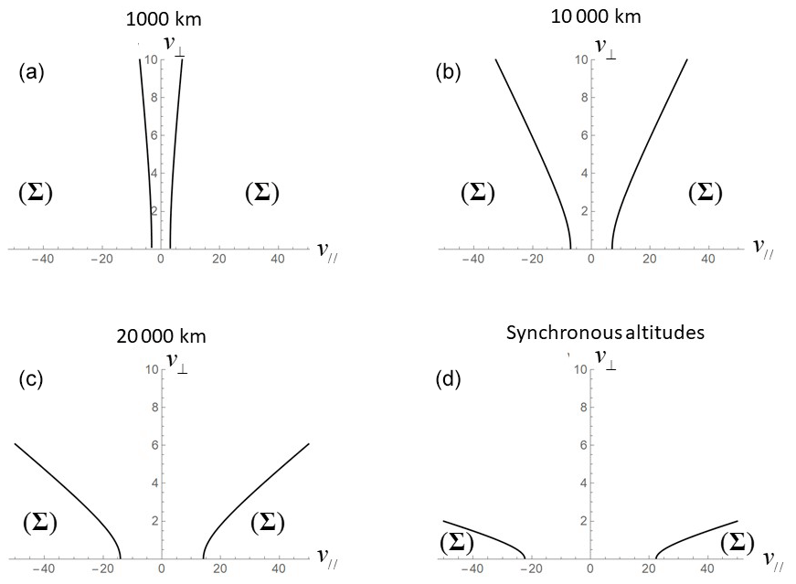
Figure 2 Regions of velocity space (Σ) occupied by the ionospheric species are shown. They were accelerated by the parallel potentials and magnetic mirror force: (a) electrons (ions) at 1000 km altitudes for parallel potentials of 10 V (−10 V), (b) electrons (ions) at 10 000 km for 50 V (−50 V), (c) electrons (ions) at 20 000 km for 200 V (−200 V), and (d) electrons (ions) at geosynchronous altitudes for 500 V (−500 V). In the velocity space, ($v_{//}$, v_⊥) is normalized by the thermal velocity of respective particles (1 eV for this case).

In Fig. 2, both the magnetic mirror force and parallel potential accelerated ionospheric sources are shown. This acceleration process moved ionospheric source plasmas labeled (Σ) to the bottom-right or to the bottom-left corner in velocity space as the altitudes increased from 1000 km to the geosynchronous altitudes. Figure 2 illustrates two cases: (1) ionospheric electrons are accelerated in downward electric fields for which field-aligned potential increased with increasing altitudes; (2) ionospheric ions are accelerated in upward electric fields for which the potential decreased with increasing altitudes. Assuming the Maxwell distribution function for velocity distributions of ions and electrons above 1000 km altitudes, in accordance with Liouville's theorem ($\mathrm{d}f/\mathrm{d}t=\mathrm{0}$) we calculate parallel and perpendicular temperatures of ionospheric species at altitudes of 1000 km, 10 000 km, 20 000 km, and geosynchronous. The velocity distribution function of ionospheric plasmas is given by

$$\begin{array}{}\text{(5)}& \begin{array}{rl}f(v_{//},v_{\perp };\mathrm{\Phi })& ={\left({\displaystyle \frac{m_q}{\mathrm{2}\mathit{\pi }k{T}_q}}\right)}^{\mathrm{3}/\mathrm{2}}\\ & \cdot \exp \left({\displaystyle \frac{m_q}{\mathrm{2}k{T}_q}}(v_{//}^{\mathrm{2}}+v_{\perp }^{\mathrm{2}})+{\displaystyle \frac{q\left|e\right|\mathrm{\Phi }}{k{T}_q}}\right).\end{array}\end{array}$$

Here, kT_q is 1 eV for ions and electrons. Electrostatic potential Φ is 0 V at the ionosphere.

The temperature of the parallel and perpendicular component (eV) is given by $\frac{m_q}{\mathrm{2}}〈v_{//,\perp }^{\mathrm{2}}〉$, where

$$\begin{array}{}\text{(6)}& 〈v_{//,\perp }^{\mathrm{2}}〉={\displaystyle \frac{{\int }_{\mathrm{\Sigma }}{v}_{//,\perp }^{\mathrm{2}}f\left(v\right){\mathrm{d}}^{\mathrm{3}}v}{{\int }_{\mathrm{\Sigma }}f\left(v\right){\mathrm{d}}^{\mathrm{3}}v}}.\end{array}$$

Integration was carried out over the velocity space (Σ) bounded by the hyperbolic curves in both the negative (earthward) and positive (tailward) velocity component in $v_{//}$.

For both ions and electrons, parallel and perpendicular temperatures $\left(\frac{m_q}{\mathrm{2}}〈v_{//}^{\mathrm{2}}〉,\frac{m_q}{\mathrm{2}}〈v_{\perp }^{\mathrm{2}}〉\right)$ initially (0.5, 1.0 eV) in the ionosphere changed to (11.3, 0.70 eV) at 1000 km where electrostatic potential was 10 V for electrons and −10 V for ions. Temperatures changed to (51.9, 0.09 eV) at 10 000 km where electrostatic potential was 50 V for electrons and −50 V for ions. When electrostatic potential further increased to 200 V for electrons and decreased to −200 V for ions at 20 000 km, temperatures changed to (202.0, 0.02 eV). At geosynchronous altitudes, temperatures changed to (502, 0.002 eV) where potential is assumed to be 500 V for electrons and −500 V for ions. Parallel potential and mirror geometry skewed the velocity space of the ionospheric source, increased parallel temperatures, and decreased perpendicular ones at altitudes above the ionosphere.

The other cases in which parallel potentials act as a potential barrier are shown in Fig. 3. In this type, dynamical trajectories filled all velocity space in $v_{//}$, and parallel temperature (0.5 eV at the ionosphere) did not change above the ionosphere up to geosynchronous altitudes, while perpendicular temperature decreased to 0.87 eV at 20 000 km and to 0.42 eV at geosynchronous altitudes. We conclude that accelerating potential raised the parallel temperature of the escaping ionospheric species. The potential barriers did not change the parallel temperature of the ionospheric source.

Figure 3 Same as Fig. 2, but parallel potential behaved as potential barriers: (a) electrons (ions) at 1000 km for parallel potentials of −10 V (10 V), (b) electrons (ions) at 10 000 km for −50 V (50 V), (c) electrons (ions) at 20 000 km for −200 V (200 V), and (d) electrons (ions) at geosynchronous altitudes for −500 V (500 V).

A brief explanation is given below as to how the local potentials that have extracted electrons and ions from the ionosphere developed at higher altitudes above the ionosphere. We note that electrons and ions traveling earthward in the left-hand side of the velocity space marked by Σ may contribute to the development of parallel potentials. In flux tubes where parallel potential accelerates electrons (ions) out of the ionosphere, the same parallel potential in the flux tubes acts as a potential barrier for ions (electrons) escaping the ionosphere. In this flux tube small-pitch-angle electrons (ions) and large-pitch-angle ions (electrons) traveling earthward generate downward (upward) electric fields by charge separation along the flux tubes of mirror geometry (Alfven and Falthammar, 1963; Persson, 1963; Stern, 1981). These potentials are global in scale and vary monotonically from the ionosphere to the Equator. However, a rate of parallel potential change (parallel electric fields) may decrease above an altitude of 10 000 km because magnetic mirror force drops rapidly in these regions.

The resultant potential distributions in the polar ionosphere and in the magnetosphere are presented in Fig. 4. Because of parallel potentials in the magnetosphere, the potential difference in the ionosphere never weakens but instead amplifies during equatorial projection.

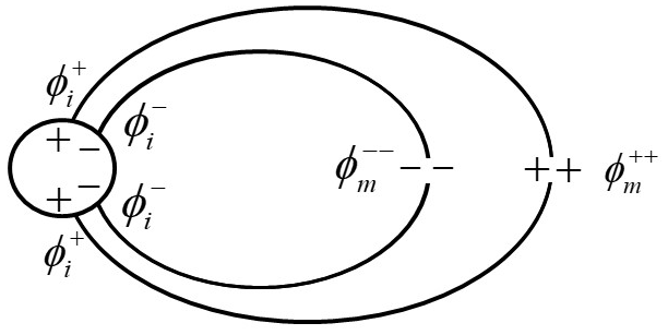
Figure 4 An equatorial projection of the ionospheric potentials (${\mathit{\varphi }}_{\mathrm{i}}^{+}$ and ${\mathit{\varphi }}_{\mathrm{i}}^{-}$) from the Southern and Northern Hemisphere is illustrated. Ionospheric potentials are positive at higher latitudes (${\mathit{\varphi }}_{\mathrm{i}}^{+}$) and negative at lower latitudes (${\mathit{\varphi }}_{\mathrm{i}}^{-}$). Parallel potential amplified potential difference in the ionosphere during the equatorial projection (${\mathit{\varphi }}_{\mathrm{m}}^{++}>{\mathit{\varphi }}_{\mathrm{i}}^{+}$, ${\mathit{\varphi }}_{\mathrm{m}}^{--}<{\mathit{\varphi }}_{\mathrm{i}}^{-}$). Earthward electric fields are produced in the plasma sheet.

4 Field-aligned current

Ions in the E layer drifted from positive potentials at higher latitudes to negative potentials at lower latitudes to discharge the imbalance produced by the mobility difference. Drift velocities of these ions (U_i⊥) may be given as

$$\begin{array}{}\text{(7)}& {\mathit{u}}_{\mathrm{i}\perp }={\displaystyle \frac{{\mathrm{\Omega }}_{\mathrm{i}}}{B{\mathit{\nu }}_{\mathrm{in}}}}{\mathit{E}}_{\mathrm{p}}.\end{array}$$

Here, Ω_i, ν_in, and E_p denote ion cyclotron frequency, ion-neutral collision frequency, and secondary polarization electric fields, respectively. Substituting mean ion cyclotron and ion-neutral collision frequencies in Eq. (7), we have ion drift velocities on the order of 5.9×10¹ m s⁻¹ for electric fields of the order of 0.1 V m⁻¹. Those drifting ions carry southward Pedersen currents of the order of 1.0 µA m⁻² in the E layer. These ionospheric currents might be redirected to the field-aligned currents at the poleward and equatorward edge of the flow channel of the current to close the 2-D current system. We therefore suggest that field-aligned currents of the order of 1.0 µA m⁻² may flow above the ionosphere in the ionospheric injection scenario. To test this hypothesis, we calculate the field-aligned currents along the dynamical trajectories using ${\mathit{J}}_{//q}=nq\left|e\right|〈v_{//}〉$, where

$$\begin{array}{}\text{(8)}& 〈v_{//}〉={\displaystyle \frac{{\int }_{\mathrm{\Sigma }}{v}_{//}f\left(v\right){\mathrm{d}}^{\mathrm{3}}v}{{\int }_{\mathrm{\Sigma }}f\left(v\right){\mathrm{d}}^{\mathrm{3}}v}}.\end{array}$$

To calculate electric currents, velocity space integration was carried out only in the positive velocity component in $v_{//}$ (traveling tailward) because those in the negative velocity component traveling earthward may be reflected in the magnetic mirror geometry and cancel the currents carried by earthward-traveling particles. The results show that ionospheric electrons at altitudes of 10 000 km (electrostatic potential is 50 V) carry downward field-aligned currents of the order of 2.0 µA m⁻² at the number density 10¹ m⁻³. This is a fraction of the background density at those altitudes (n=10⁹ m⁻³). We conclude that upward-flowing ionospheric electrons may close Pedersen currents at the poleward edge of the channel, while upward-flowing ionospheric ions (oxygen ions) at the equatorward edge of the channel carried 0.69 nA m⁻² at the same altitudes (electrostatic potential is −50 V) and with the same number density of electron currents. Electric currents carried by the ions are smaller than those carried by electrons by the mass ratio of electrons and ions if the temperatures of electrons and ions are the same. They cannot provide sufficient current density to close the Pedersen currents. Therefore, electrons from the magnetosphere are necessary for closing the Pedersen currents at the equatorward edge of the channel.

5 Summary and discussion

Despite the ionospheric dynamo processes driven by the neutral wind, local electrostatic fields that form in less than 1 min may be expected in ionospheric injection because electrons participate in the dynamo process. Electrons are pumped up towards negative electrodes at lower latitudes by ExB drift. The drift generates poleward Hall currents flowing in an opposite direction in the equatorward electric field. The westward electric fields of the magnetospheric origin may generate the ionospheric dynamo. The dynamo process yielded plasma injections arising out of the ionosphere (evaporation of ionospheric plasmas) and generated preferentially field-aligned potentials below 10 000 km.

Although the substorm onset would be triggered initially by the magnetospheric convection enhancement (arrival of the dipolarization front from the tail), we suggest that activation of the ionospheric dynamo (auroral onset) may be controlled by the intensity of westward electric fields penetrating the auroral ionosphere. Because electric fields penetrating the ionosphere are stronger in a dark hemisphere (lower Pedersen conductance) than in a sunlit hemisphere (higher Pedersen conductance) (Saka, 2019), auroras are more active in the dark hemisphere (Newell et al., 1996).

Field-aligned potentials were generated in the magnetosphere such that the ionospheric potentials were amplified during their equatorial projection. This means that the ionosphere responded to the initial dipolarization by returning the southward electric fields to the dipolarization region in the magnetosphere. The southward electric fields in the ionosphere that became earthward electric fields in the plasma sheet further displaced the dipolarizing flux tube eastward, which relaxed the radial inhomogeneity and intensified the dipolarization (Saka, 2020). This positive feedback loop may happen in the magnetosphere and ionosphere systems with asymmetric development of the dipolarization region in the dawn–dusk directions. This asymmetry may be related to the difference in the onset time of the substorm current wedge in dawn and dusk sectors (Nagai, 1991). In this scenario, Harang discontinuity (HD) is generated in the auroral ionosphere through the ionospheric injection processes and projected back to the magnetosphere to modify the existing magnetospheric convection patterns (e.g., Artemyev et al., 2016). This scenario differs from the proposal of Erickson et al. (1991) and Liu and Rostoker (1991) that an asymmetric plasma pressure distribution introduced in the equatorial plane of the nightside magnetosphere produces HD in the polar ionosphere.

It was suggested that the deformation velocity of an aurora is about 5–8 km s⁻¹ regardless of its scale size (Oguti, 1975a, b). Oguti (1975b) noted from his observations that large-sale auroras (∼ 1000 km) such as bulge or surge are the sum of small-scale auroras (∼ 3 km) such as rays. Small-scale auroras that may be equivalent to the minimum size of the electrostatic potential of negative charge are fundamental to the MI coupling processes in the ionospheric injection scenario.