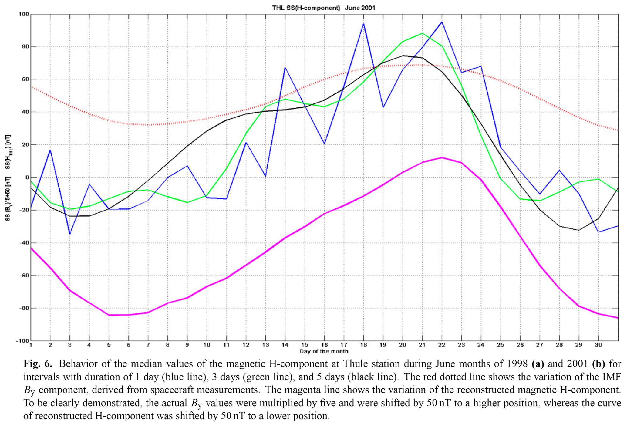
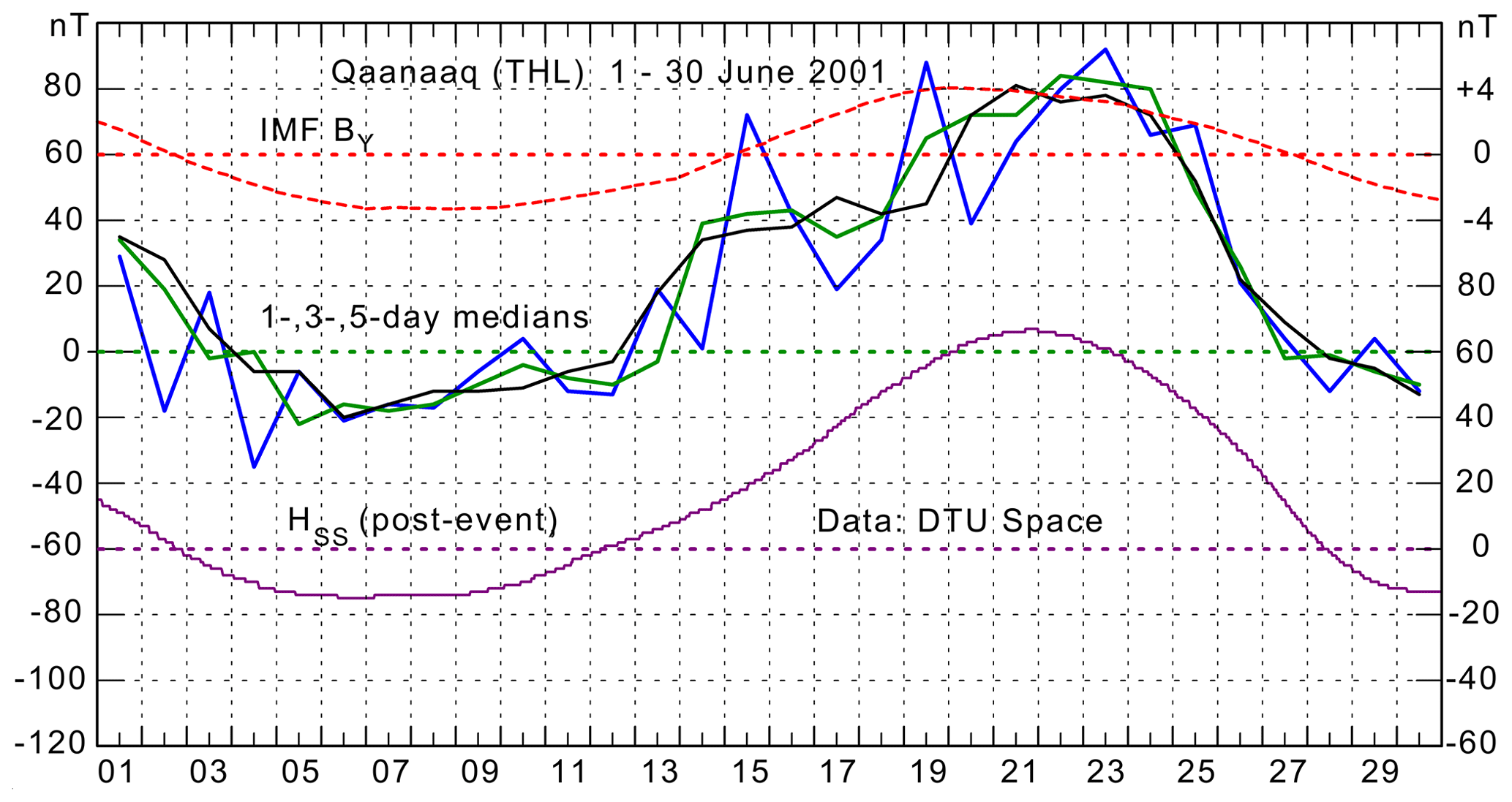
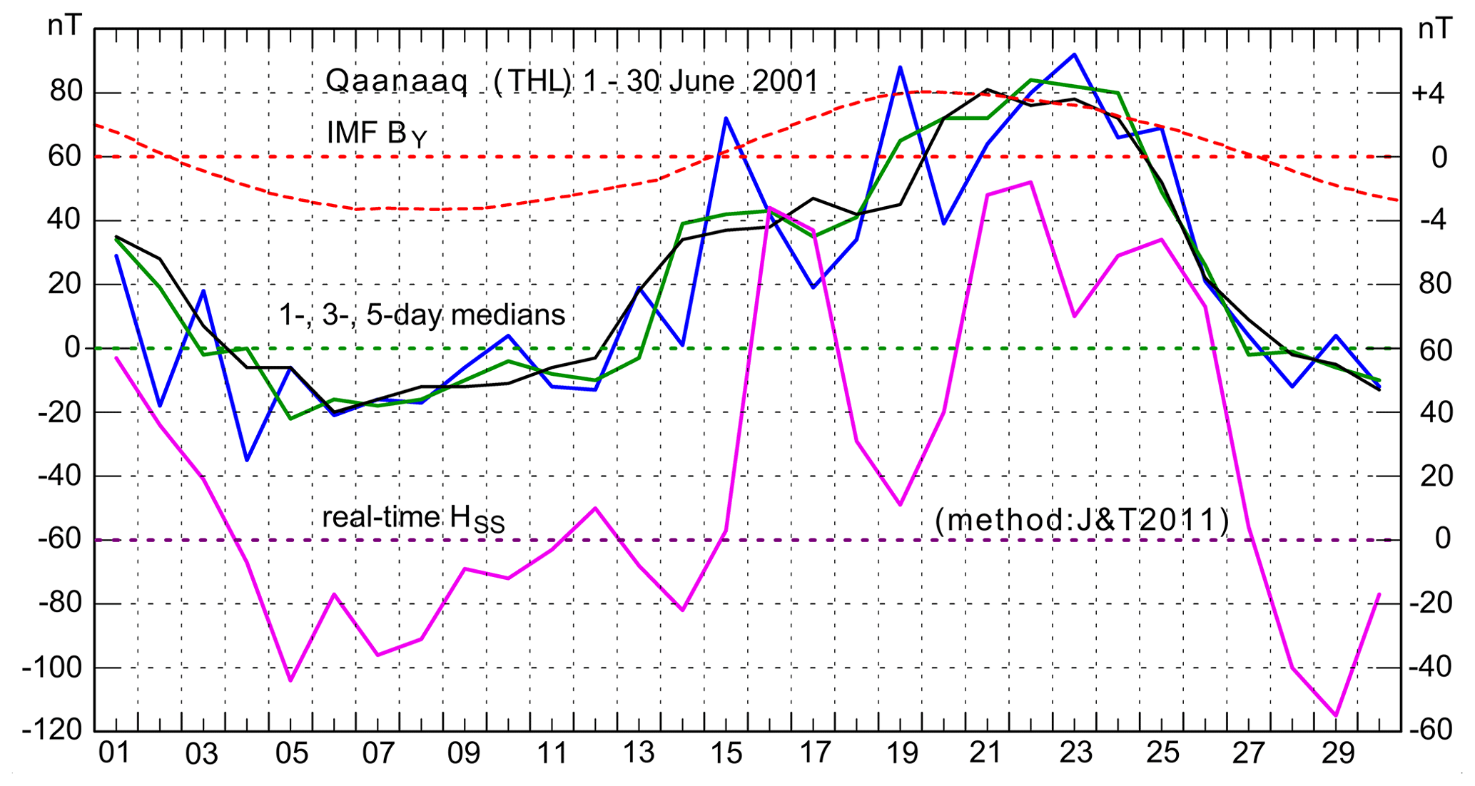
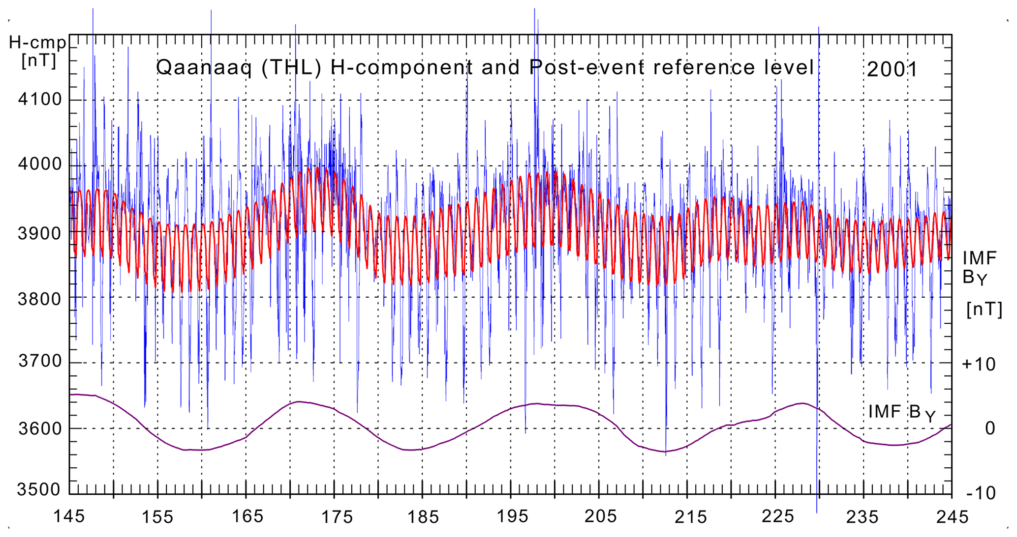
Comment on “Identification of the IMF sector structure in near-real time by ground magnetic data” by Janzhura and Troshichev (2011)

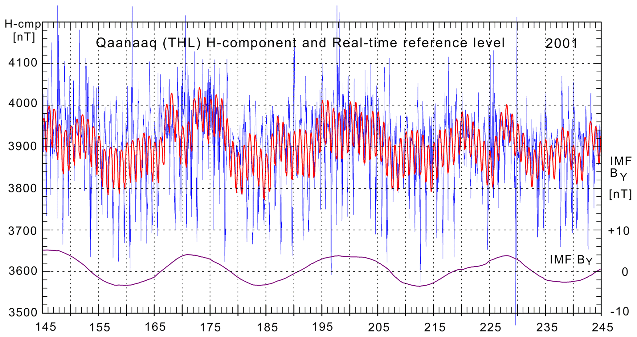
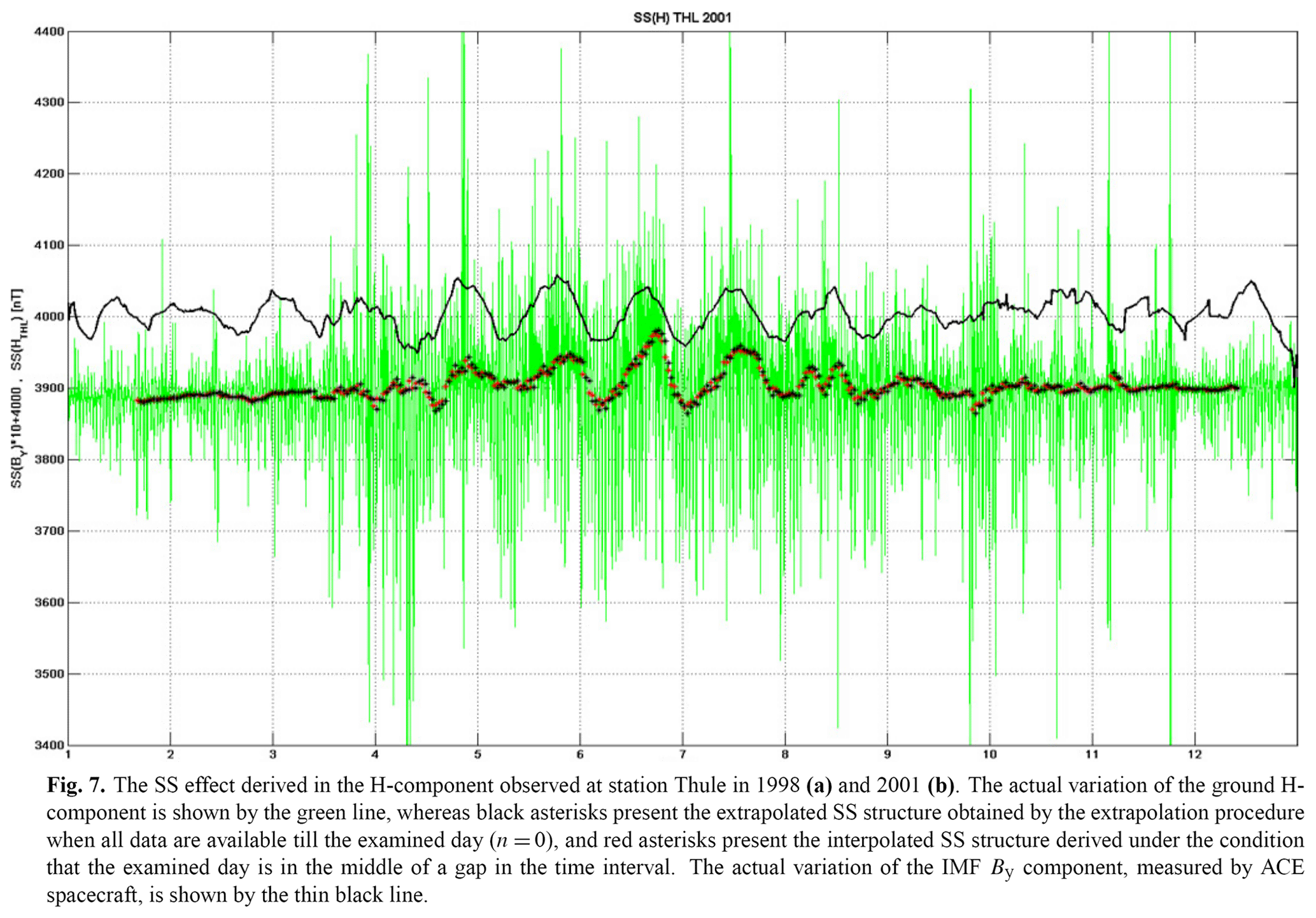
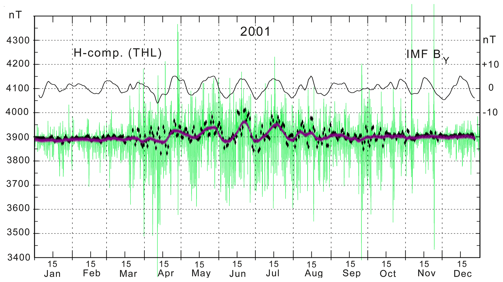
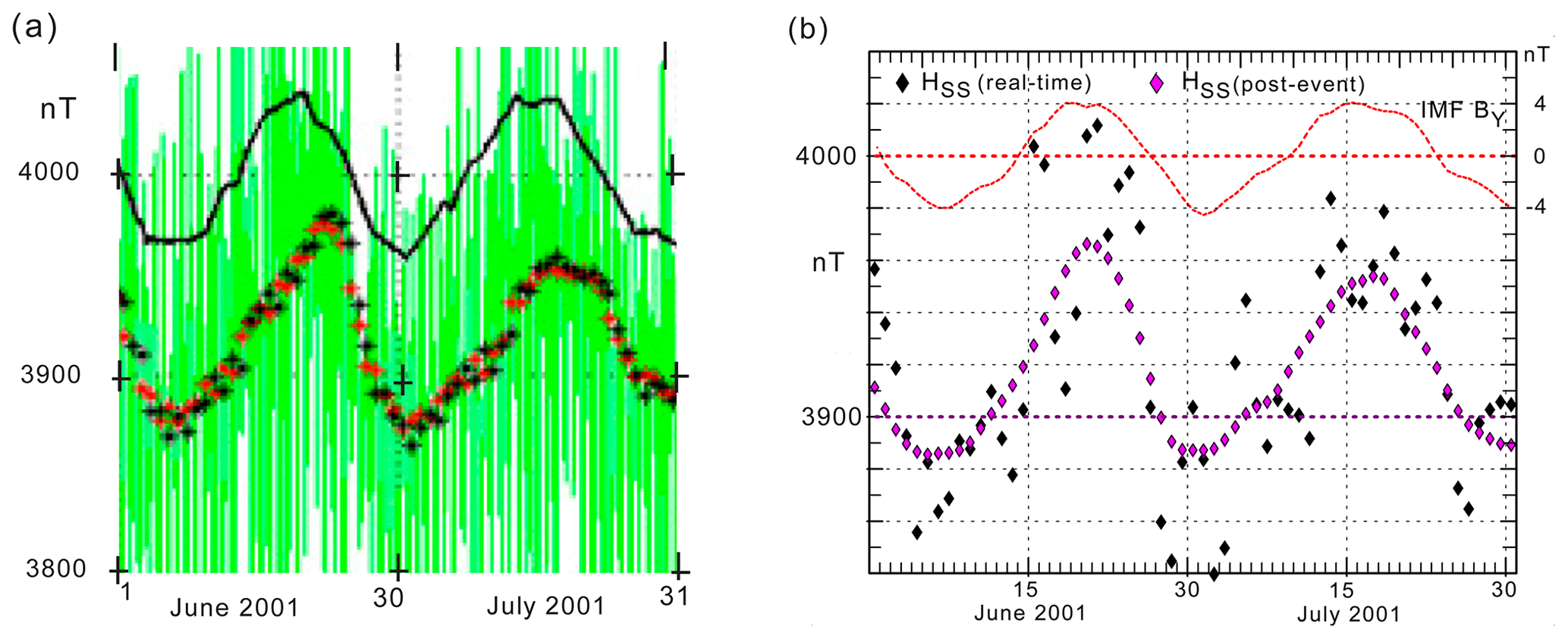
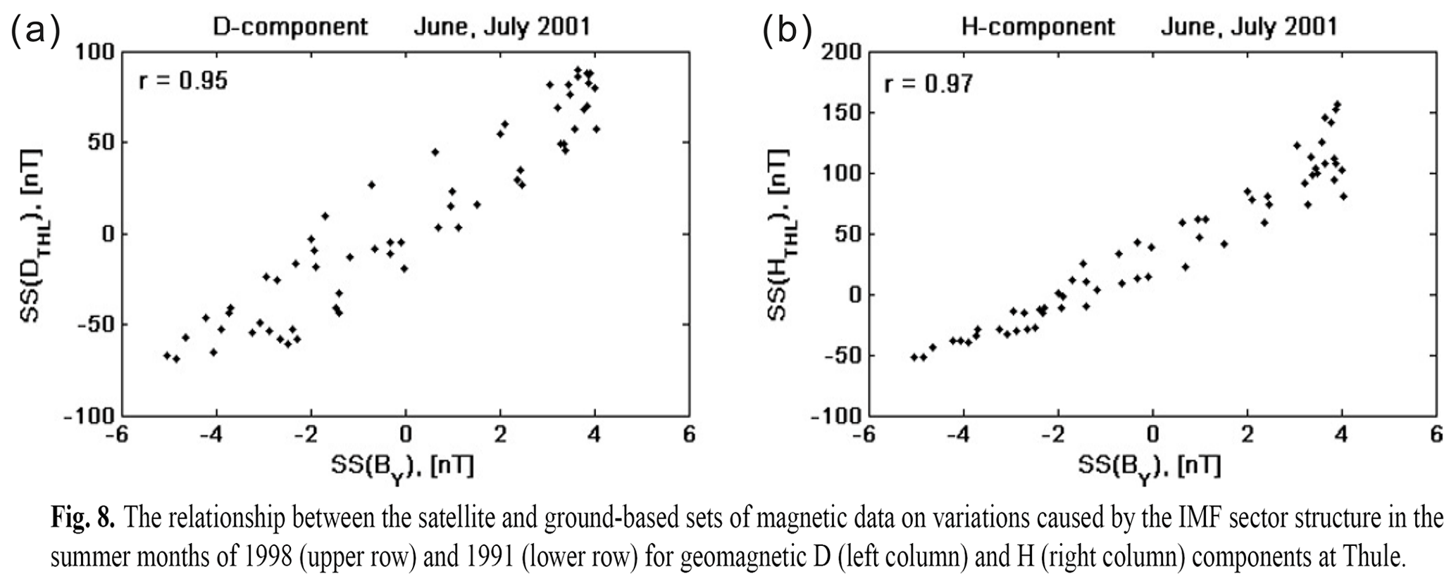
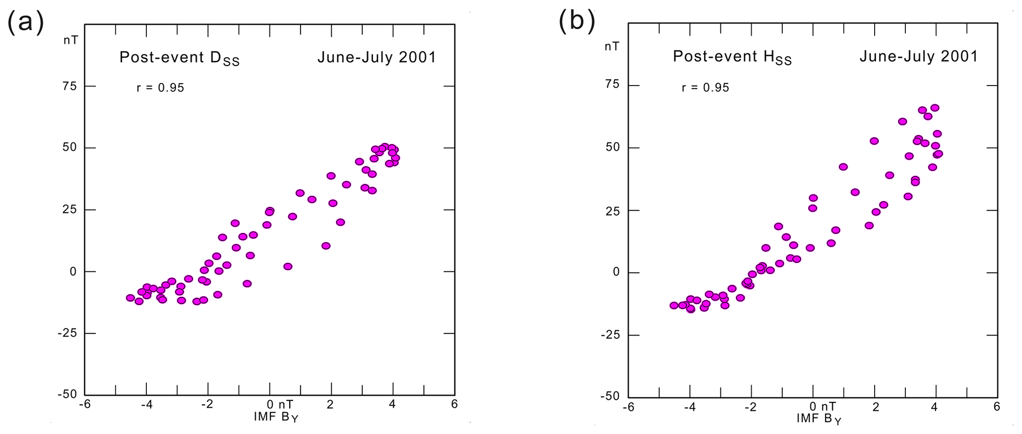
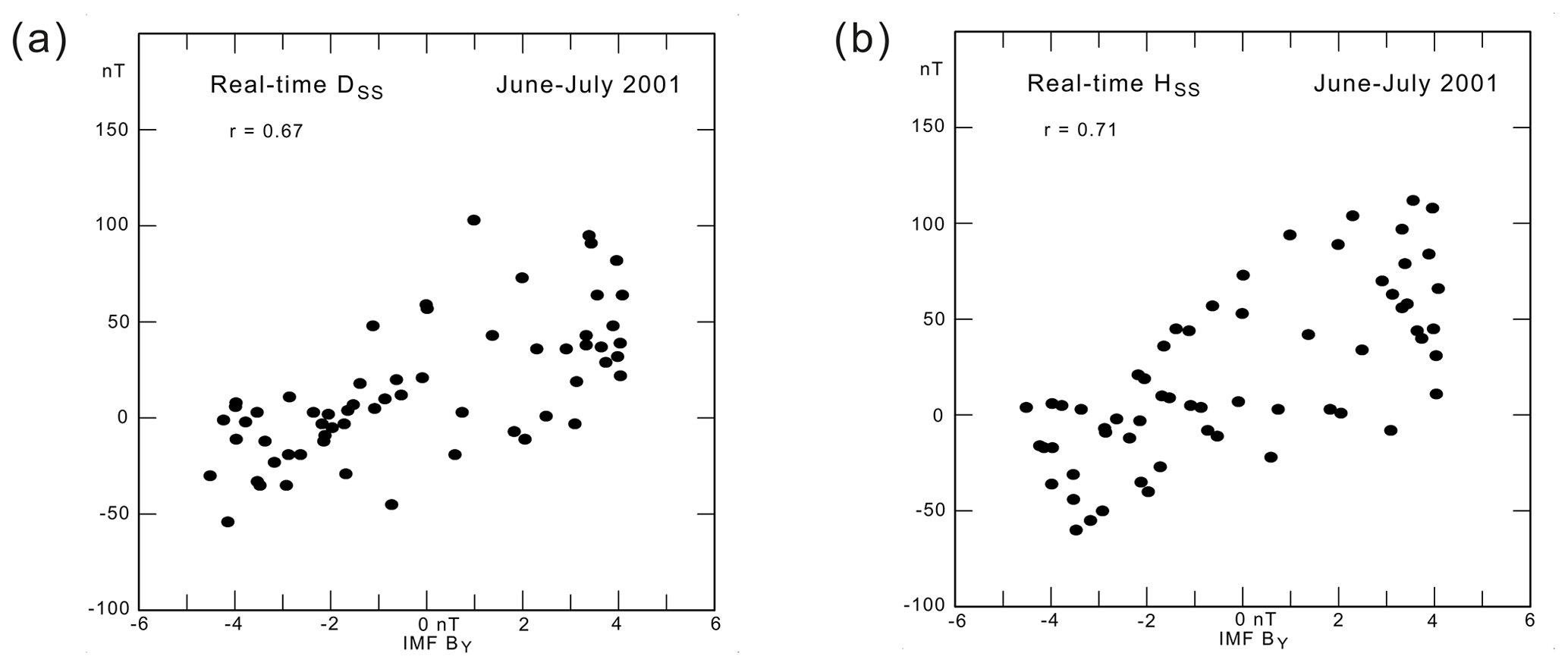
The only published description of the solar wind sector (SS) term used for the reference level in the post-event and real-time derivation of the Polar Cap (PC) indices, PCN (Polar Cap North) and PCS (Polar Cap South), in the version endorsed by the International Association for Geomagnetism and Aeronomy (IAGA) is found in the commented publication, Janzhura and Troshichev: Identification of the IMF sector structure in near-real time by ground magnetic data, Annales Geophysicae, 29, 1491–1500, 2011. Actually, the publication has served as a basis for the index endorsement by IAGA in 2013. However, neither the illustrations nor the results presented there have been derived by the specified near real-time method. Figures 1, 6, 7, and 8 display values derived by post-event calculations based on daily medians smoothed over 7 d centred on the day of interest. Figures 2, 3, and 4 display observed values smoothed over 7 d, while the remaining Fig. 5 displays averages over 4 months. In summary, there are strong disagreements between indications in the title, abstract, and statements in the text compared to the actual results and their illustrations.

1 Introduction

The derivation of the Polar Cap (PC) indices, PCN (Polar Cap North) based on Qaanaaq data and PCS (Polar Cap South) based on Vostok data, in the versions endorsed by the International Association for Geomagnetism and Aeronomy (IAGA) in Resolution no. 3 (2013) is to a large extent based on the methods described in Janzhura and Troshichev (2011): Identification of the IMF sector structure in near-real time by ground magnetic data (hereinafter J&T2011) (and its replicate in Troshichev and Janzhura, 2012, hereinafter T&J2012). This work provides the only published description of the solar wind sector (SS) term related to the Y component, IMF B_Y, of the interplanetary magnetic field (IMF). The SS terms are derived from daily median values of the recorded magnetic field components and added to the index reference level in the post-event or near real-time versions. For post-event PC index calculations, the SS terms are derived from 7 d averaging of daily median values of the recorded magnetic data. For the near real-time calculations, the SS terms are derived from cubic spline-based forward extrapolation of past median values.

Figure 1 THL H component (where THL represents station Qaanaaq, formerly Thule). The 1 d (blue line), 3 d (green), and 5 d (black) median values are shown. Resulting H_SS terms (magenta line) are shown on a scale shifted 50 nT downward for clarity. Smoothed IMF B_Y multiplied by 5 and shifted 50 nT upward is shown with the red line. (Reproduced from Fig. 6b of Janzhura and Troshichev, 2011, including caption.)

Figure 2 THL 1, 3, and 5 d medians are shown on the left scale. Post-event H_SS terms are displayed (magenta line) on the lower right scale. The data were supplied from DTU Space (http://space.dtu.dk, last access: 10 April 2021). Smoothed IMF B_Y values (red line) are added on the upper right scale (data from OMNIWeb, http://omniweb.gsfc.nasa.gov, last access: 10 April 2021).

However, the method is invalid since it assumes that the IMF B_Y-related effects originating at the dayside cusp region can be compensated for by using a daily median-based SS term at all local hours. Instead, the addition of this singular term to the index reference level generates unfounded positive or negative PC index contributions at different observatory positions along its daily path with respect to the polar cap ionosphere. The solar wind sector “compensation”, typically, generates unfounded contributions to the PC indices at the nightside although the real IMF B_Y effects on polar magnetic fields at the night side are usually very small. Correspondingly, the compensation might have little effect on PC indices at the dayside although the cusp-related IMF B_Y effects maximize there.

Figure 3 THL 1, 3, and 5 d medians are shown on left scale. Simulated real-time H_SS terms (magenta line) on the lower right scale. H_SS values were calculated by following exactly the procedure in J&T2011 (Stauning, 2018). Smoothed IMF B_Y values are added on the upper right scale (OMNIWeb).

Figure 4 PCN reference level (thick line) superimposed on recorded H-component data (thin line). (Reproduction of Fig. 1 of Janzhura and Troshichev, 2011, with caption included.)

An example case gave an unfounded change of 2.45 mV/m (magnetic storm level according to Troshichev and Sormakov, 2018) at local midnight and hardly any effect at noon at 4 nT amplitude in smoothed IMF B_Y values, which is a common occurrence (Stauning, 2015).

Figure 5 Post-event (final) PCN reference level values (red line) supplied from DTU Space superimposed on recorded H-component data (blue line). IMF B_Y values (magenta line) on the lower right scale are added at the bottom of the diagram for reference (after Stauning, 2015).

Figure 6 Simulated real-time PCN reference level (red line) derived by rigorous use of the J&T2011 procedure superimposed on recorded H-component data (blue line). IMF B_Y values are added at the bottom of the diagram.

2 Calculation of IMF B_Y-related solar wind sector term

The commented publication, J&T2011, holds (pp. 1496–1497) a step-by-step procedure quoted below for near real-time calculations of IMF B_Y-related solar wind sector (SS) terms by forward cubic spline-based extrapolation of past median values.

Keeping in mind this specification, the 3 d smoothing averages of the median values were subjected to the interpolation procedure including the following steps:

1. median values for magnetic components H and D are derived for 4 intervals of days preceding with the exception of the current day (n=0):

   • r1 = F [for interval from n−3 to n−1 d]

   • r2 = F [for interval from n−5 to n−3 d]

   • r3 = F [for interval from n−7 to n−5 d]

   • r4 = F [for interval from n−9 to n−7 d];

2. piecewise polynomial form of the cubic spline interpolant for r1, r2, r3, and r4 segments is determined;

3. termination of this form related to day n=0 is examined as representative of the SS effect for the current day, even if this day is disturbed.

The procedure is repeated each subsequent day. Results of the procedure – the variation of the reconstructed magnetic H component is presented by the magenta line in the same Fig. 6, the reconstructed H-component curve being shifted by 50 nT to a lower position.

Figure 7 Presentation of 1 year's THL H-component data (green line) with superimposed near real-time (black) and post-event H_SS values (red asterisks). IMF B_Y values are added (black line). (Reproduced from Fig. 7b of Janzhura and Troshichev, 2011, with caption included.)

Figure 8 THL H-component data with superimposed simulated real-time (black) and post-event (magenta diamonds) values of H_SS. Note the large scatter of the real-time (black diamonds) data. IMF B_Y values are added (black line) on the upper right scale.

Figure 9 (a) Detailed plot of the June–July section of Fig. 7 from Janzhura and Troshichev (2011). Note the almost continuous transition from black to red diamonds. IMF B_Y values are included (black line). (b) Details of Fig. 8. Note the large scatter in the black diamonds (simulated real time) away from the post-event magenta diamond symbols. IMF B_Y values are added for reference (red line).

Figure 10 Reproduction of Fig. 8b from Janzhura and Troshichev (2011) (including caption). Relations between daily average IMF B_Y values and solar wind sector (a) D_SS and (b) H_SS values. Note that scale values are by some error (misprint) too large by a factor of 2.

Thus, it is stated (p. 1497) that this procedure was used to derive the smoothly varying display of the H-component SS term (magenta line) in their Fig. 6 using magnetic data from Qaanaaq (THL) for the interval 1–30 June 2001, here reproduced in Fig. 1 and recalculated in Fig. 2. However, the statement concluding the quoted procedure is incorrect. The SS term (H_SS) displayed in Fig. 6 of J&T2011 could not have been generated by the quoted near real-time procedure. The smoothed magenta curve for H_SS is not a real-time version but derived by using the post-event method based on daily median values smoothed over 7 d with the actual day at the middle. Figure 2 presents the post-event (“final”) H_SS values derived by the PCN index suppliers at the Danish Space Research Institute (DTU Space).

Figure 11 Display of post-event (final) solar wind sector terms, D_SS and H_SS, supplied from DTU Space vs. daily average IMF B_Y values. Note that the scales are reduced by a factor of 2 from those of Fig. 10 to correct the scaling errors in Fig. 8 of J&T2011.

Figure 12 Display of simulated real-time solar wind sector terms, D_SS and H_SS, calculated by using the procedure in J&T2011, p. 1496, plotted vs. daily average IMF B_Y values.

Values of the solar wind sector term, H_SS, derived by adhering rigorously to the above-quoted “near-real time” procedure (including the cubic spline-based forward projection) are displayed by the jagged curve in magenta line in Fig. 3.

The similarity between the H_SS curves in Figs. 1 and 2 and the large difference with respect to the simulated real-time H_SS values in Fig. 3 derived from cubic spline-based extrapolation of past median values implies that the display in Fig. 6 of J&T2011 (Fig. 4.15 of T&J2012), contrary to the statement in pp. 1496–1497, was actually generated by using post-event calculations with smoothed averages of 7 d daily median values.

3 Use of the solar wind sector (SS) term in reference level for PC indices

The IMF B_Y-related solar wind sector effects on the convection patterns generate changes in the PC index response to the merging electric fields. The solar wind sector (SS) term was implemented in the derivation of PC index reference levels by J&T2011. The SS term from their Fig. 6 has been added to the quiet day variation (QDC) with slowly (seasonally) varying amplitude calculated by the method published in Janzhura and Troshichev (2008) to generate the June section (days 152–182) of the reference level displayed by the solid line superimposed on the 1 min H-component values displayed in their Fig. 1. The remaining part of the reference levels has no doubt been generated by the same method reproduced here in Fig. 4 (including caption) and recalculated in Fig. 5. However, using the near real-time H_SS version generates the jagged reference level displayed in red solid line superimposed on the H-component values displayed in faint blue line in Fig. 6.

The close similarity of the reference level (thick line) in Fig. 4 with that of Fig. 5 and the strong difference with respect to the real-time reference level in Fig. 6 implies that the “QDC” in Fig. 4 was actually derived by the post-event (final) calculation method (7 d smoothing of daily median H-component values) like the method used for Fig. 5.

4 The SS effects throughout a year (2001).

Figure 7b in J&T2011 (Fig. 4.16b in T&J2012) displays the H component recorded at Qaanaaq (THL) throughout year 2001. The IMF B_Y-related H_SS values have been superimposed on the recordings. According to the description, the black asterisks present near real-time values, while the red asterisks present post-event values. It appears that the two sets of symbols merge to form a smooth continuous curve. However, contrary to the description in text and figure caption, both symbol series have been generated by post-event calculation methods (averaged daily median values).

Recalculated values are displayed in Fig. 8 where the post-event symbols (magenta diamonds) merge to form a continuous broad trace of H_SS values. The scattered near real-time symbols (black diamonds) have been calculated by using rigorously the J&T2011 near real-time procedure quoted above. Figure 9a and b provide more detailed comparisons of the values displayed in Figs. 7 and 8.

It is evident from Figs. 8 and 9b that the real-time and post-event methods generate quite different values of the IMF B_Y-related solar wind sector terms, H_SS. The set of red asterisks in Figs. 7 and 9a, no doubt, present post-event (smoothed daily median) values, while the black set in Figs. 7 and 9a, against the statements in the text and in the figure caption, could not present near real-time values but must have been derived by post-event smoothing.

5 Identification of solar wind sector structure in near real time

Figure 8b of J&T2011 reproduced here in Fig. 10 displays close relations between solar sector terms D_SS and H_SS and daily average IMF B_Y values. These relations are assumed to enable the possible identification of the IMF sector structure in near real time (title of the publication).

D_SS and H_SS values for the summer months, June–July 2001, provided by DTU Space are displayed in Fig. 11a and b (left and right). The values have been calculated from the 7 d averaged daily median D- and H-component values (magenta symbols) using the post-event method.

The corresponding near real-time values of D_SS and H_SS, for June–July 2001, have been calculated by rigorous use of the above-quoted near real-time procedure from J&T2011. The results are displayed in Fig. 12a and b.

The similarity between the diagrams of Fig. 11 definitely constructed by post-event calculations (at DTU Space) and that of Fig. 10 indicates beyond doubt that the latter have been derived by post-event methods. From the post-event processing displayed in Figs. 10 and 11, the D- and H-component solar wind sector terms appear highly correlated (r=0.95, 0.97) with the daily mean IMF B_Y values. Thus, they could be used to estimate past IMF B_Y levels and signs with good probability from archived data. However, the objective according to the title and abstract of the paper was to estimate IMF B_Y in near real time.

Compared to the D_SS and H_SS solar wind sector terms derived by post-event calculations displayed in Figs. 10 and 11, the corresponding solar wind sector terms generated by using real-time processing are much less well correlated with the daily average IMF B_Y values (r=0.67, 0.71). The relations displayed in Fig. 12 by the scattered D_SS and H_SS values derived by using near real-time methods could hardly be used to determine the actual IMF B_Y magnitude level and sign with any certainty, which was the main scope of the J&T2011 publication.

6 Summary and conclusion

The commented paper, J&T2011, and its replica in Troshichev and Janzhura (2012) are significant since, along with the publications Troshichev et al. (2006) and Troshichev et al. (2011) held in chapter 4 of Troshichev and Janzhura (2012), they form the basis for the derivation procedures (Matzka, 2014; Nielsen and Willer, 2019) applied for calculations of Polar Cap (PC) index values in the near real-time and post-event (final) versions endorsed by IAGA Resolution no. 3 (2013).

However, neither the illustrations nor the results presented in J&T2011 have been derived by the specified near real-time method. All the illustrations and results presented in Figs. 1, 6, 7, and 8 display values derived by post-event calculation methods based on daily median values smoothed over 7 d centred on the day of interest. Figures 2, 3, and 4 display observed values smoothed over 7 d, while the remaining Fig. 5 displays averages over 4 months.

In summary, there is strong disagreement between indications in the title, abstract, statements in the text, and captions, as well as in the presentation of results, compared to recalculations by rigorous use of the presented near real-time procedure. Thus, it is concluded to caution against uncritical use of the methods and results presented in the commented publication by Janzhura and Troshichev (2011).

References

Janzhura, A. S. and Troshichev, O. A.: Determination of the running quiet daily geomagnetic variation, J. Atmos. Sol.-Terr. Phys., 70, 962–972, https://doi.org/10.1016/j.jastp.2007.11.004, 2008.
Janzhura, A. S. and Troshichev, O. A.: Identification of the IMF sector structure in near-real time by ground magnetic data, Ann. Geophys., 29, 1491–1500, https://doi.org/10.5194/angeo-29-1491-2011, 2011.
Matzka, J.: PC_index_description_main_document_incl _Appendix_A.pdf, DTU Space web portal, available at: https://doi.org/10.11581/DTU:00000057, 2014.
Nielsen, J. B. and Willer, A. N.: Restructuring and harmonizing the code used to calculate the Definitive Polar Cap Index, Report from DTU Space, available at: https://doi.org/10.11581/DTU:00000057, 2019.
Stauning, P.: A critical note on the IAGA-endorsed Polar Cap index procedure: effects of solar wind sector structure and reverse polar convection, Ann. Geophys., 33, 1443–1455, https://doi.org/10.5194/angeo-33-1443-2015, 2015.
Stauning, P.: A critical note on the IAGA-endorsed Polar Cap (PC) indices: excessive excursions in the real-time index values, Ann. Geophys., 36, 621–631, https://doi.org/10.5194/angeo-36-621-2018, 2018.
Troshichev, O. A. and Janzhura, A. S.: Space Weather monitoring by ground-based means, Springer Praxis Books, Heidelberg, https://doi.org/10.1007/978-3-642-16803-1, 2012.
Troshichev, O. A. and Sormakov, D. A.: PC index as a proxy of the solar wind energy that entered into the Magnetosphere: 3. Development of magnetic storms, J. Atmos. Sol.-Terr. Phys., 180, 60–77, https://doi.org/10.1016/j.jastp.2017.10.012, 2017.
Troshichev, O. A., Janzhura, A. S., and Stauning, P.: Unified PCN and PCS indices: method of calculation, physical sense and dependence on the IMF azimuthal and northward components, J. Geophys. Res., 111, A05208, https://doi.org/10.1029/2005JA011402, 2006.
Short summary
The commented publication by Janzhura and Troshichev (2011) constitutes an essential part of the basis for the IAGA endorsement by Resolution 3 (2013) of PC index calculations. However, there is strong disagreement between indications of near real-time methods in the title, abstract, statements in the text, and figure captions, as well as in illustrations of results in the article compared to results from recalculations of the relations by rigorous use of the presented near real-time procedure.