Stratospheric influence on the mesosphere–lower thermosphere over mid latitudes in winter observed by a Fabry–Perot interferometer

In this paper, we study the response of the mesosphere–lower thermosphere (MLT) to sudden stratospheric warmings (SSWs) and the activity of planetary waves (PWs). We observe the 557.7 nm optical emission to retrieve the MLT wind and temperature with the only Fabry–Perot interferometer (FPI) in Russia. The FPI is located at the mid latitudes of eastern Siberia within the Tory Observatory (TOR) at the Institute of Solar-Terrestrial Physics of the Siberian Branch of the Russian Academy of Sciences (ISTP SB RAS, 51.8^∘ N, 103.1^∘ E). Regular interferometer monitoring started in December 2016. Here, we address the temporal variations in the 557.7 nm emission intensity as well as the variations in wind and temperature measured during the 2016–2020 winters. Both SSWs and PWs appear to have equally strong effects in the upper atmosphere. When the 557.7 nm emission decreases due to some influences from below (SSWs or PWs), the temperature increases significantly, as does its variability. The dispersion of zonal wind does not show significant PW- and SSW-correlated variations, but the dominant MLT zonal wind reverses during major SSW events simultaneously with the averaged zonal wind at 60^∘ N in the stratosphere.

1 Introduction

At present, it is well accepted that dynamic processes in various atmospheric layers interact. The main mechanism for this interaction is the vertical propagation of atmospheric waves on various temporal and spatial scales. The main role of the atmospheric waves is energy and momentum transport from the lower atmosphere to the overlying layers, as they propagate. During dissipation in the middle and upper atmosphere, the waves deposit their energy and momentum, thus affecting the thermal balance and circulation of the atmosphere. Hence, the propagation and dissipation of atmospheric waves is one of the main mechanisms responsible for the energy and dynamic interaction among the lower, middle, and upper atmosphere (Yiğit and Medvedev, 2015).

The mesosphere–lower thermosphere (MLT) is defined as the atmosphere region between about 60 and 110 km in altitude. It constitutes the upper part of what is often referred to as the middle atmosphere (10 to 110 km) (Andrews et al., 1987). Observations have shown that the closest relationship between the lower and upper atmospheric layers exists in winter and early spring (Vincent, 2015). The vertical interaction between the atmospheric layers is especially obvious during sudden stratospheric warmings, SSWs (Dowdy et al., 2007; Jacobi et al., 2009). SSWs are significant and global events that are observed in winter in both hemispheres of the Earth (Varotsos, 2002, 2003). In our paper, we analyse the atmosphere dynamics during the winter season, focusing on SSW events. Many previous studies have addressed this topic. Below, we summarize the relationship between the background wind and tidal variations in the MLT during stratosphere warming. The main signature of all winter disturbances in the MLT circulation is a significant weakening and often inversion (east-to-west) of the zonal wind for several days (Danilov et al., 1987). This feature is especially well observed at mid-latitude observatories (Limpasuvan et al., 2016). At polar latitudes, the zonal circulation is less stable; therefore, in some years, the response from the SSW in the dynamics of the MLT may be expressed differently. Most often, the zonal wind reverses westward, and the tides intensify during SSWs (Bhattacharya et al., 2004). Although SSWs are observed in the polar stratosphere, the response in the MLT background winds is recorded at equatorial and tropical observatories (Sridharan et al., 2012). In Laskar and Pallamraju (2014), the authors propose a compelling idea about the existence of a meridional circulation cell in MLT winds during SSW events, which enables the atomic oxygen transport from high to low latitudes. However, the literature does not provide reliable general conclusions of the meridional wind response at mid latitudes. The MLT meridional wind response to the dynamics of the lower layers differs with different observatories. This may be due to the fact that the background meridional wind is generally smaller than the background zonal wind in the upper atmosphere.

Like the results of numerous studies show, stratospheric warming has a significant effect on the amplitudes and phases of the MLT tidal oscillations. In Portnyagin and Sprenger (1978), the authors divided the tide variations during SSWs into two types. In the Type-1 variations, the amplitude of the semidiurnal tide increases significantly and exceeds the amplitude of the diurnal oscillation that is also larger than usual during this period. Disturbances of the Type-2 tidal variations are more complex in their temporal structure and are less common (about 30 %). The semidiurnal tide amplitude, in this case, increases shortly (from several hours to a day) and acquires a value close to the diurnal tide amplitude that does not change significantly. The present-day analysis of tides and SSWs confirms this point of view (Pedatella and Liu, 2013). Monitoring the upper atmosphere over Siberia has been performed since 1976 through various methods. Over 1976–1996, in eastern Siberia, the MLT wind was monitored by receiving signals from separated radio reception of broadcasting stations in the long-wavelength range (Vergasova and Kazimirovsky, 2010). From the study (Vergasova and Kazimirovsky, 2010), over eastern Siberia, the zonal wind at the MLT heights in winter is generally westward. Over Badary (51^∘ N, 105^∘ E), during stratospheric warming, as a rule, the zonal wind at the MLT heights was shown to weaken or change direction from west to east. There were cases when changes in the amplitude and phase of the semidiurnal tide occurred during SSWs. Monitoring the temperature regime in the Siberian region was performed by the hydroxyl emission spectral observations at the Institute of Solar-Terrestrial Physics of the Siberian Branch of the Russian Academy of Sciences (ISTP SB RAS) Tory (TOR) Observatory (Medvedeva and Ratovsky, 2017; Medvedeva et al., 2014). Observations during SSWs included a significant variation in the OH and O₂ emission intensities, a decrease in the atmosphere temperature, and an increase in wave activity. In this paper we will summarize the observations accumulated over 4 years, building upon our previous studies of wind and temperature at this site (Zorkaltseva et al., 2019, 2020).

Long-term (covering several years and more) observations of the MLT region temperature and wind are sparse, especially within the Siberian region close to the SSW emergence and evolution. Analysis of such observations is useful for understanding and predicting global circulation and for forecasting middle and upper atmospheric models. Our measurements using the Fabry–Perot interferometer enable us to simultaneously evaluate the MLT temperature and wind speed. In this paper, we address four winter periods of observations of the upper atmosphere and compare the measurements with the stratosphere dynamics.

2 Data and method

We analyse the data from the ISTP SB RAS Fabry–Perot interferometer located at the TOR in the Republic of Buryatia. Figure 1 shows the map with the instrument location.

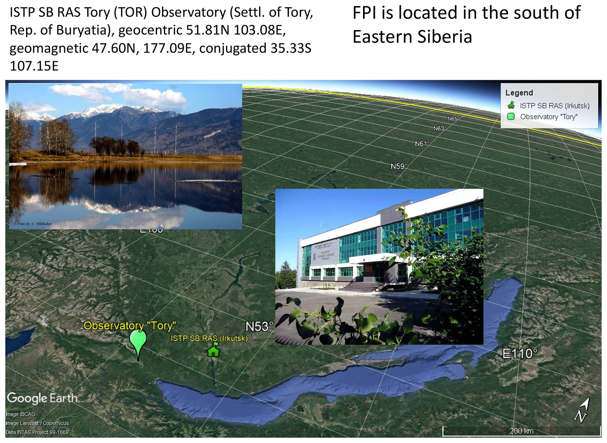
Figure 1 This © Google Earth map shows the location of the Fabry–Perot interferometer at the Tory Observatory and the Institute of Solar-Terrestrial Physics (ISTP).

The Fabry–Perot interferometer (FPI) conducts regular spectrometric observations of the natural airglow lines in the nighttime atmosphere. Precise spectral analysis enables the observation of the Doppler shift of a single line, which characterizes the velocity for the corresponding radiating component of the atmosphere along the observation's line of sight. The combination of the Doppler shifts obtained in different directions within the medium enables us to reconstruct the full vector of the wind horizontal velocity, assuming this vector is not changing during the observation interval. The line broadening provides us with an estimate of the temperature (Vasilyev et al., 2017). In this paper, we address the data on the behaviour of the zonal wind and the temperature obtained by using the 557.7 nm line emission originating at about 90–100 km over the Earth's surface. The FPI is an optical instrument; therefore, measurements are possible only in the dark, on moonless nights, when there are no clouds within the FPI field of view. Due to this, the data have periodic (daily, lunar) and aperiodic (cloudiness, technical failures) gaps. In this paper, we analyse the night-averaged values for the 557.7 nm emission intensity (I), temperature (T), and zonal wind speed (U) as well as the standard deviations of those values during each night.

To study the stratosphere dynamics, we used the ECMWF ERA5 climate archive (Hersbach et al., 2020). As per the SSW criteria established by the WMO, we utilize parameters such as the zonal average air temperature along 80^∘ N and zonal average values of the wind zonal component along 60^∘ N at the 10 hPa height on a 2.5×2.5^∘ grid. We also studied the dynamics of planetary waves with zonal wavenumbers 1 (PW1) and 2 (PW2). We addressed all the characteristics at the 1 and 10 hPa heights.

3 Results and discussion

3.1 Sudden stratospheric warmings

Figure 2 shows the daily zonal mean zonal wind at 60^∘ N (blue) and the temperature at 80^∘ N (red) obtained from the ERA5 reanalysis dataset for 1 October 2016 through 31 March 2017 at the 10 hPa height (solid) and at 1 hPa (dotted). We see that two stratospheric warmings were observed with a peak on 1 February (251 K) and 27 February (251 K), SSW1 and SSW2, respectively, marked by dotted vertical lines in the figure. The grey rectangles show the SSW duration. As a criterion for the warming onset, we consider a day with a sharp temperature increase (more than 10^∘ d⁻¹). We consider the end of the sharp (about 2^∘ d⁻¹) temperature decrease to be the end of the SSW. SSW1 started on 20 January and ended on 12 February. SSW2 started on 23 February and ended on 5 March. As per the World Meteorological Organization (WMO) standard criteria, two minor warming events were observed during the 2017 winter. Note that the warming at the 1 hPa height was significant, and the zonal circulation reversed. This may be important for analysing vertical interactions that we address below.

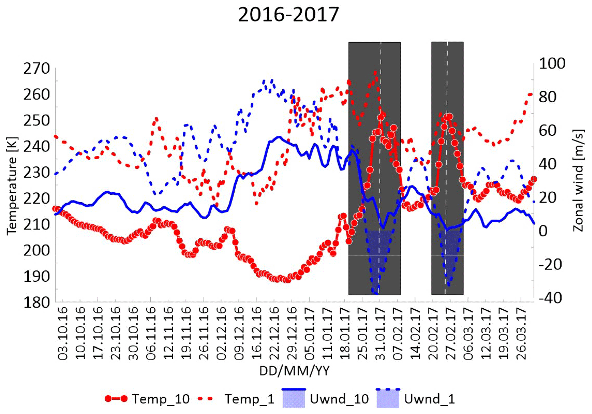
Figure 2 Zonal mean of the zonal wind at 10 hPa (blue solid line) and 1 hPa (blue dotted line) and zonal mean temperature at 10 hPa (red solid line) and 1 hPa (red dotted line) obtained from the ERA5 reanalysis dataset for October 2016 through March 2017.

In the introduction, we discussed that waves, including planetary waves, are the cause of vertical interaction in the atmosphere. Periods of increase in the planetary wave amplitude in the stratosphere are not always accompanied by the SSW evolution. Therefore, we address (and mark on the plots) the periods of planetary wave amplitude increase without SSWs and compare them with the MLT dynamics in the next section. In the figures, we mark the PW1 amplitude increase above the average value for each winter with a light grey rectangle. Figure 3 shows that, in early November 2016, there was a significant PW1 amplitude increase that persisted for about a month.

Figure 3 Amplitude of planetary wave 1 at 10 hPa (solid line) and PW2 amplitude at 10 hPa (dotted line) for October 2016 through March 2017.

The SSW spatial structure may also be important for the upper atmosphere response. We analysed temperature maps during warmings. As an example, we give a temperature map on the SSW maximum day (Fig. 4) at 10 hPa. In the 2016–2017 winter, both SSW cases evolved in the Eastern Hemisphere, and the warming centre was located near the FPI location.

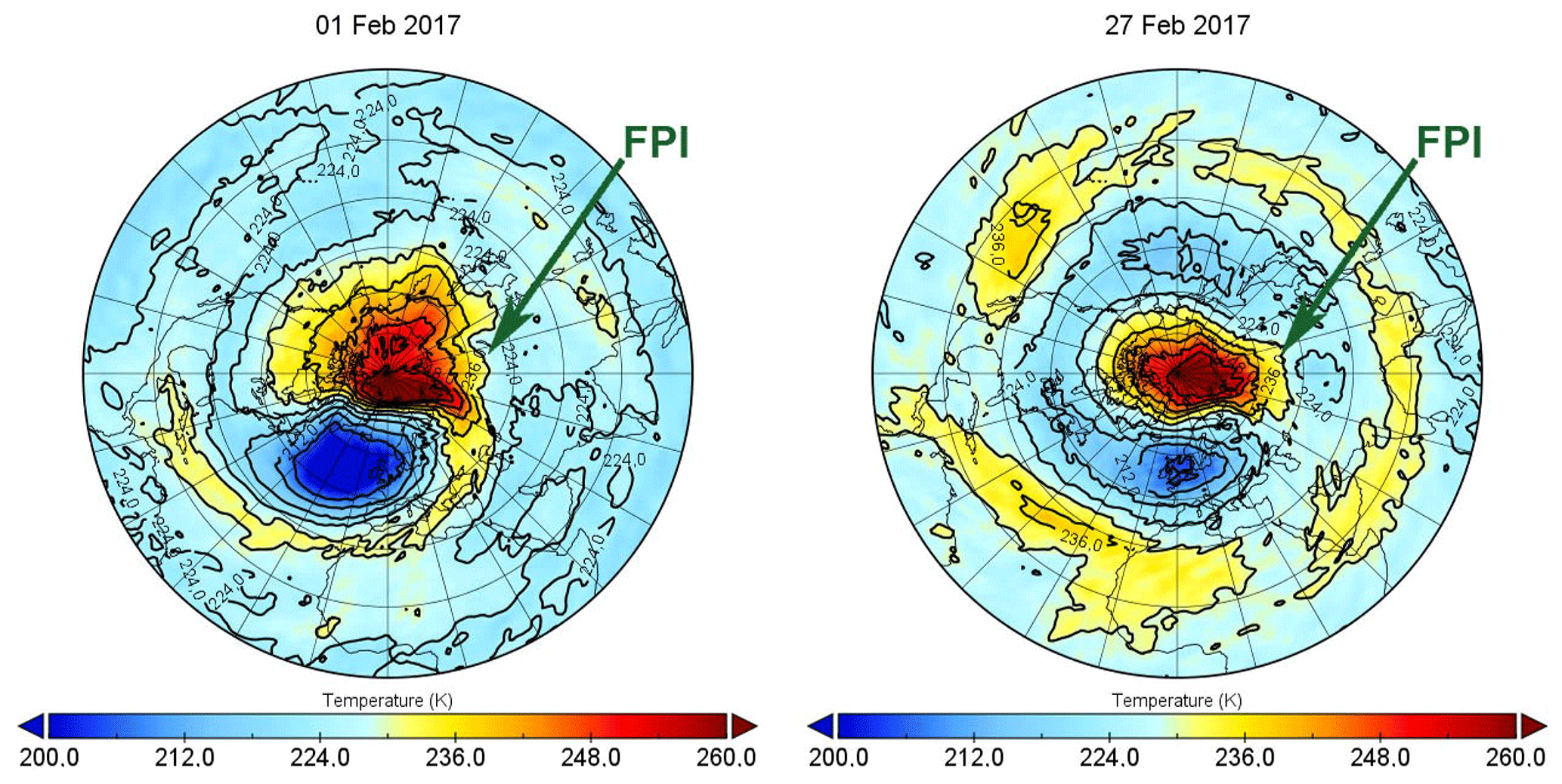
Figure 4 Distribution of temperature at 10 hPa in stereographic projection at the SSW maximum. Green arrow shows the FPI location.

In the 2017–2018 winter, there was one SSW case that started on 10 February and ended on 2 March. The maximal temperature was 246 K by 18 February. In Fig. 5, we can see that the warming was major, and the zonal wind inversion was observed at 10 and 1 hPa. The warming predominantly evolved in the Western Hemisphere over America, and the FPI was at the edge of the SSW (Fig. 7). Note that the 1 hPa temperature decreased during the SSW. Before the SSW onset, two PW1 increases were observed in the stratosphere. A PW1 increase was noted in December 2017 as well as from mid-January to early February. Figure 6 shows these periods with light grey rectangles.

Figure 5 Same as Fig. 2 but October 2017 through March 2018.

Figure 6 Same as Fig. 3 but October 2017 through March 2018.

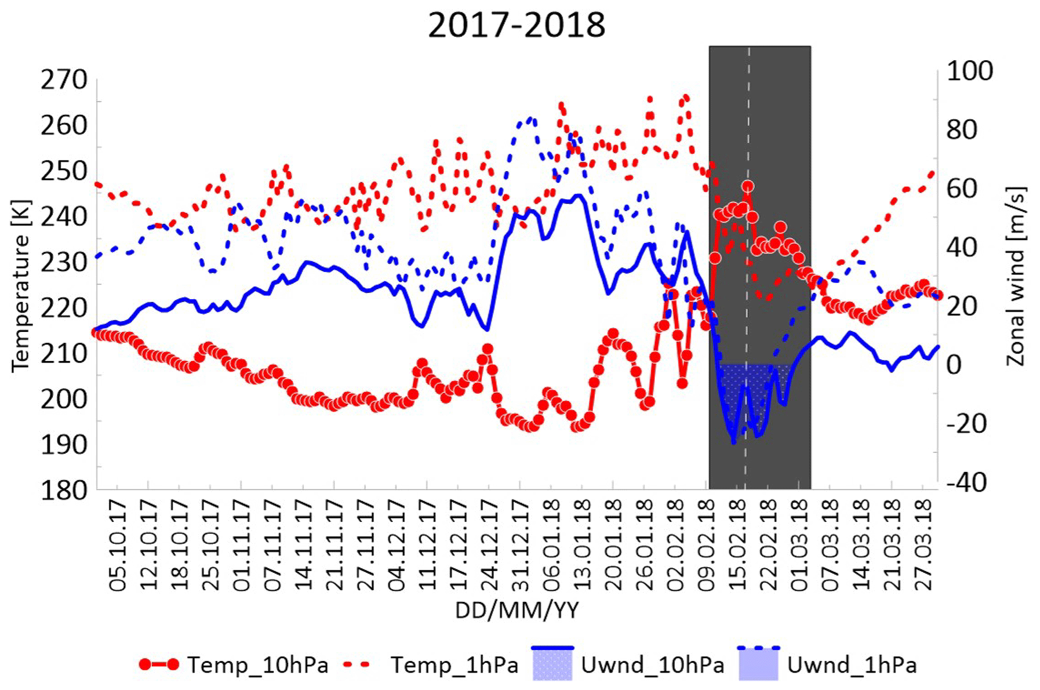
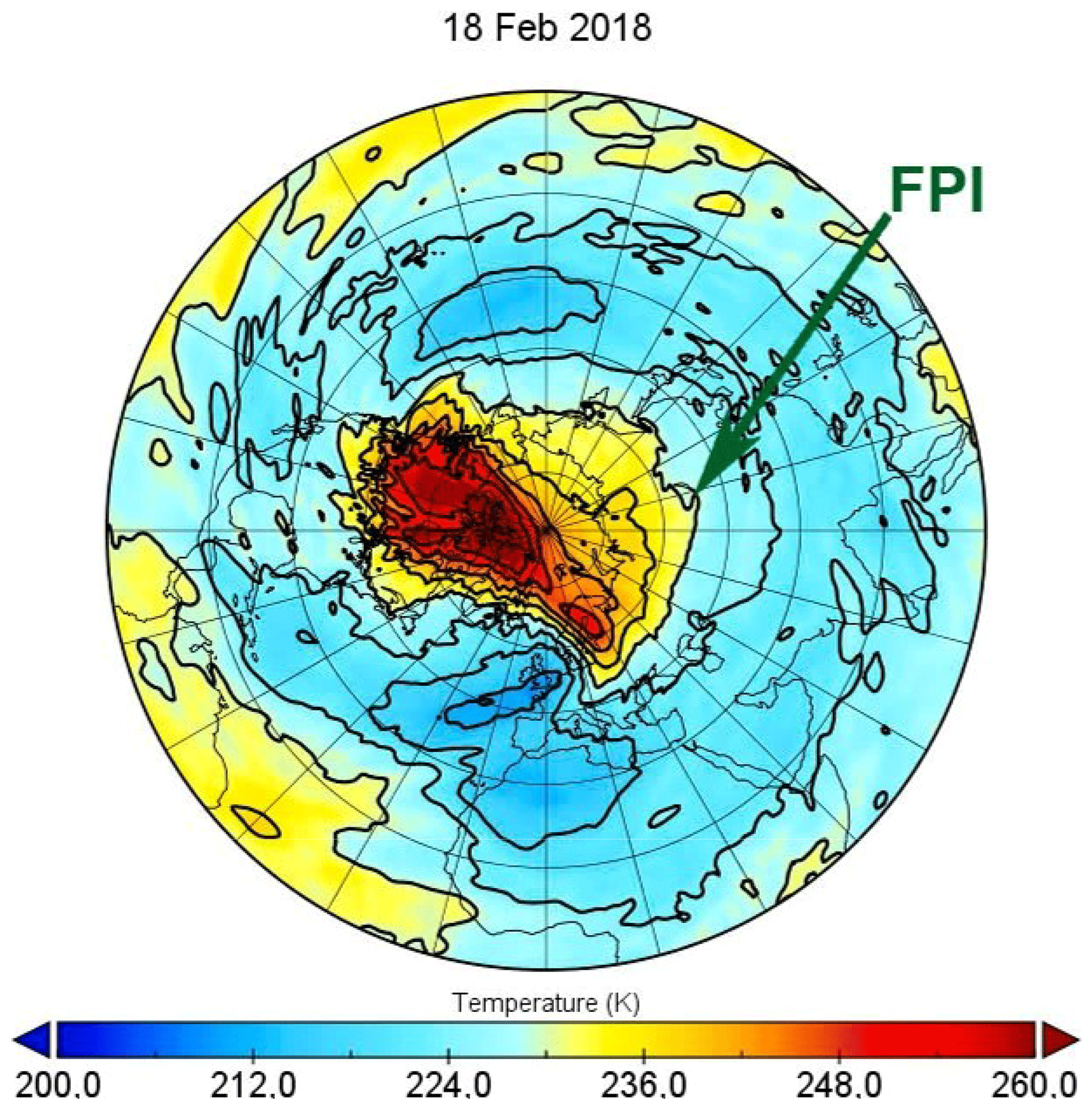
Figure 7 Same as Fig. 4.

In the 2018–2019 winter, one SSW case was observed. The SSW emerged on 22 December and lasted until 19 January. The maximal temperature during that warming was 248 K on 29 December (Fig. 8). A temperature increase was observed throughout the stratosphere. During the warming, the wind changed its direction to westward. The FPI was within the area of warming during that winter (Fig. 8). In November and December 2018, increased PWs were observed; we marked those periods with light grey rectangles in Fig. 10. The latter shows that the warming covered the entire polar region, with the interferometer site being influenced by warm air in the stratosphere.

Figure 8 Same as Fig. 2 but October 2018 through March 2019.

Figure 9 Same as Fig. 3 but October 2018 through March 2019.

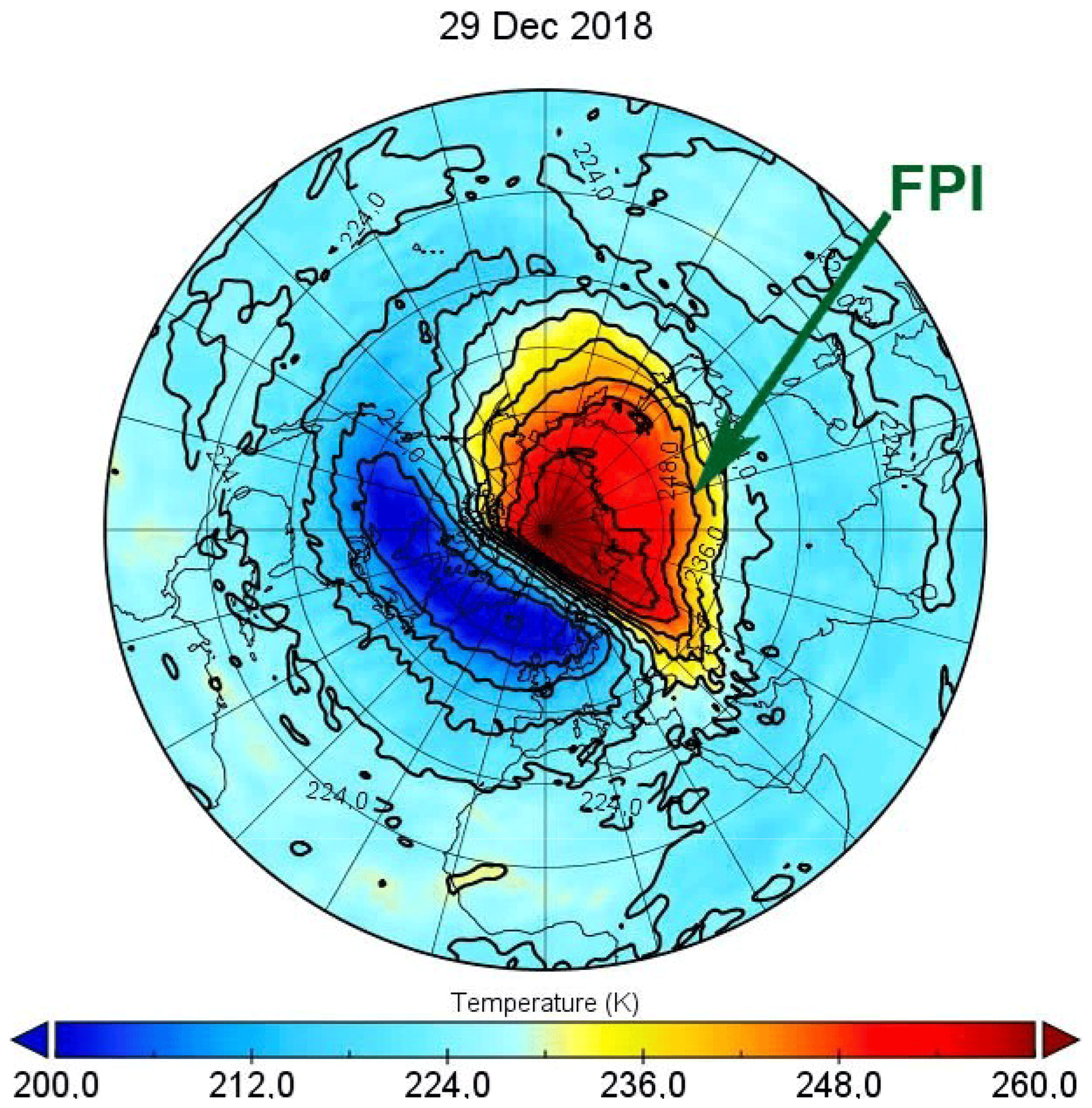
Figure 10 Same as Fig. 4.

In the 2019–2020 winter, there were two stratospheric warming cases shifted to a later date. The first warming was minor and lasted from 30 January through 20 February with a maximal temperature of 239 K on 5 February. SSW2 caused a significant temperature increase at 10 and 1 hPa; at 1 hPa, the zonal wind reversed. The SSW2 lasted from 9 March through 28 March, and the maximal temperature was 255 K on 23 March. Two PW increases preceded the SSW evolution in the stratosphere; we note that these planetary waves were the largest seen during the entire 2016–2020 period (Fig. 12). During both SSW events, the FPI was within the warming area (Fig. 13).

Figure 11 Same as Fig. 2 but October 2019 through March 2020.

Figure 12 Same as Fig. 3 but October 2019 through March 2020.

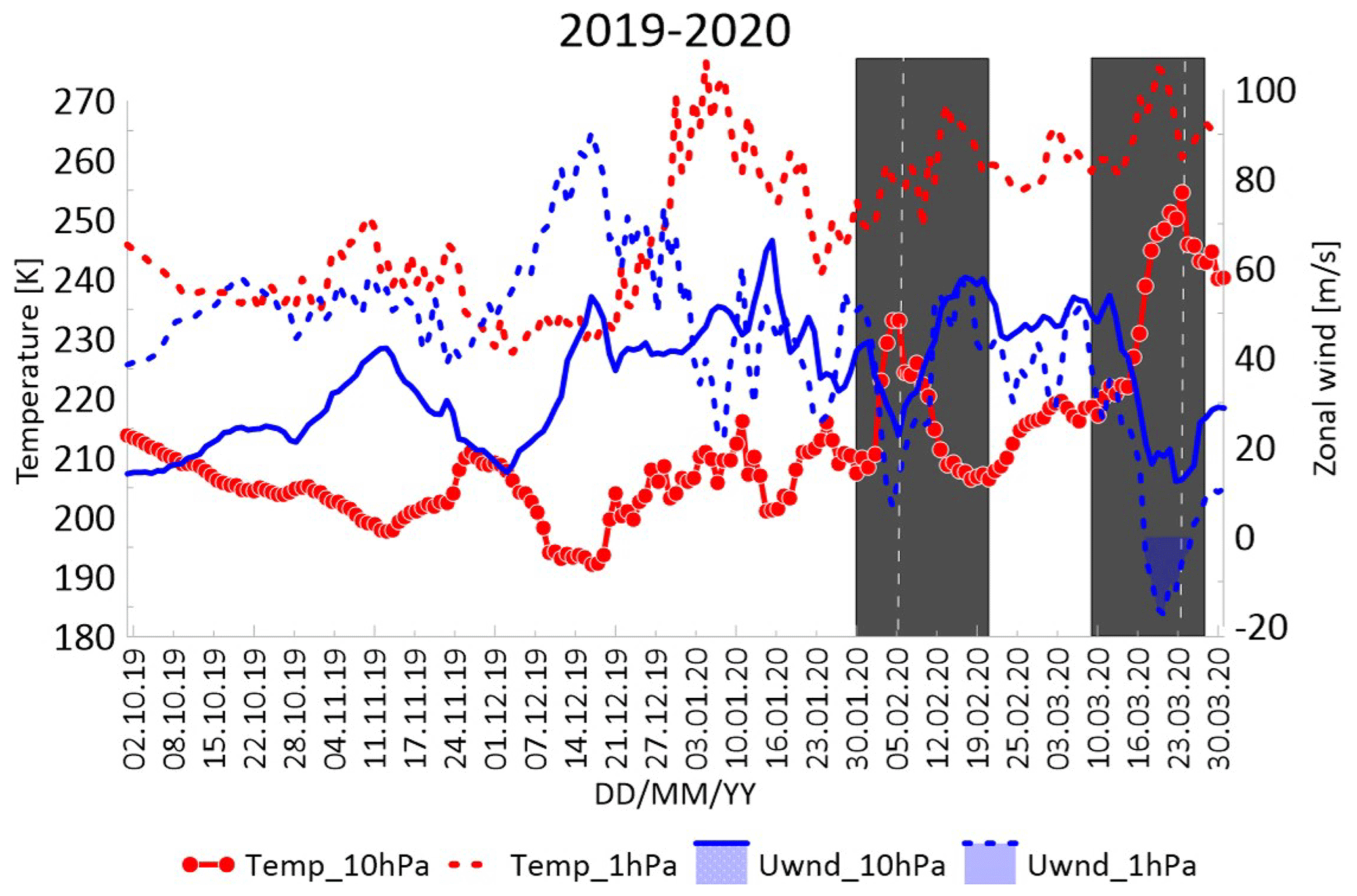
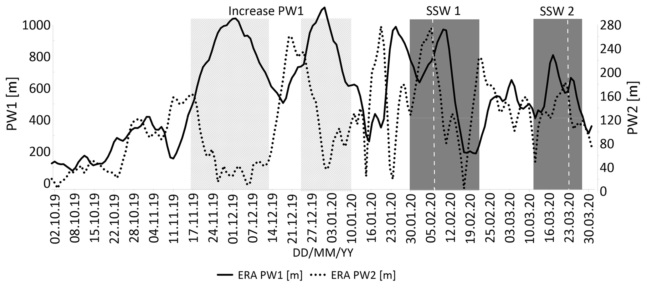
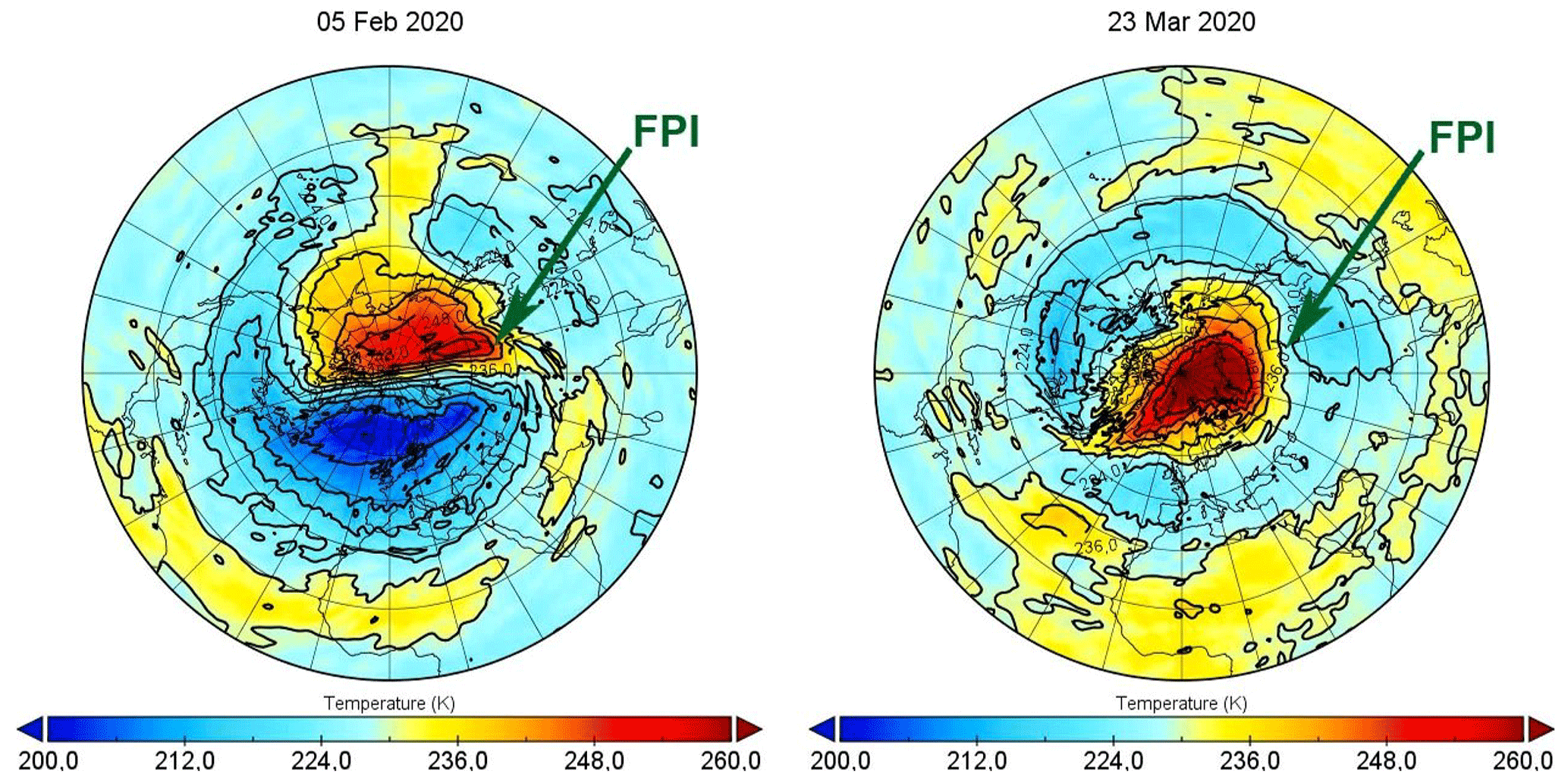
Figure 13 Same as Fig. 4.

3.2 FPI-measured average night values of the 557.7 nm emission and temperature

In this section, we address the FPI-measured mean nighttime values for the 557.7 nm emission, temperature, and zonal wind. In Figs. 14–15, we note the SSWs periods (grey rectangle), the day of maximal SSW temperature (dotted white vertical line), and the periods of increased planetary wave activity (light grey rectangle). The amplitudes of planetary waves were calculated along 60^∘ N with zonal wave numbers 1 and 2 (PW1 and PW2, respectively) from the ERA5 data.

The general pattern in Fig. 14 is a decrease in airglow emission and an increase in temperature during an active stratosphere. However, in each winter there were peculiarities in this pattern. For example, in winter 2016–2017, at the beginning of SSW1, an increased temperature was observed, but the emission did not decrease from its average value. During the maximum of SSW1, a decrease in emission and an increase in temperature are clearly visible. The influence of SSW2 in 2016–2017, in our opinion, manifested itself in the MLT dynamics at the end of the warming. Figure 14 shows that on 6 March (27 February was the maximum of SSW2), the emission was minimum and the temperature was maximum. In the interval between SSW1 and SSW2, the airglow was maximum and the temperatures were normal. On the day of the maximum stratospheric warming in 2017–2018, we see that the airglow of the green line has sharply decreased and the temperature in the MLT has increased. We also see two periods of higher temperatures and lower emissions in December and January. These periods were due to the increased activity of PW in the stratosphere. The same pattern occurred during the SSW in 2018–2019. The maximum stratospheric warming was observed simultaneously with low airglow and high temperatures in the MLT. Two periods of increased activity of planetary waves in the stratosphere caused changes in the upper atmosphere. The only winter that does not correspond to the general pattern of the relationship between the stratosphere and MLT is 2019–2020. In 2019–2020, there were two cases of SSWs, and they were observed at a later date than SSWs usually occur. During the SSW1 period, there were technical problems with the FPI, and there were no observations. During SSW2, before its maximum development, we see that the airglow has decreased, and the temperature has increased. However, between SSW1 and SSW2, the emission was also minimal, and the temperatures were high, even higher than during SSW2. We are unable to interpret these unexpected observations. There may have been some other factors that influenced the MLT. In the future, we will collect statistics and analyse such cases more carefully.

We have analysed six cases of SSWs and five cases of increased PW; in most cases, during an active stratosphere, the emission of the green line decreases and the MLT temperature rises. The temperature rises may be explained by different heights of the emitting layer. The green line can be radiated from heights with higher temperatures and reach values of up to 250 K, because the temperature height gradient over the mesopause can be extremely high (up to 10 K km⁻¹). Analysing the temperature behaviour obtained with the 557.7 nm line, we can conclude that the green line emission shifted upward into the thermosphere and the emission rate decreased due to the inverse temperature dependence of the Barth mechanism (Barth, 1961). In addition to SSW, the planetary wave activity impacts the MLT dynamics. The PW activity most often precedes SSWs, but it may appear long before the warming onset and cause a response (often stronger than SSW) in the MLT temperature regime.

Preliminary analysis of the full vector of the wind velocity showed that obvious responses to the SSW and PW events exist only for the zonal wind. However, this does not mean the absence of response from both the vertical and meridional winds to the lower atmosphere dynamics. We think that this should be investigated in a separate study. In this section, we address only the strongest and most obvious response of the zonal wind to SSWs and PWs, obtained during the data analysis. The zonal wind shows a pronounced change during warmings. Like in the stratosphere, the eastward wind reverses to westward in the MLT. Moreover, the stronger the wind inversion in the stratosphere, the stronger the wind inversion in the MLT. To analyse the effect of the stratosphere on the MLT wind, it is important to consider not only the standard 10 hPa height for SSW, but also the 1 hPa dynamics. For example, two 2017 SSW cases were minor as per the WMO classification. However, during these warmings at 1 hPa, the westward wind intensified significantly. This was the reason for the wind inversion at the MLT heights. The 2018–2019 warming was major, but at 1 hPa, there was no wind inversion. Also, we see that the zonal wind only weakened and did not reverse at the MLT altitudes.

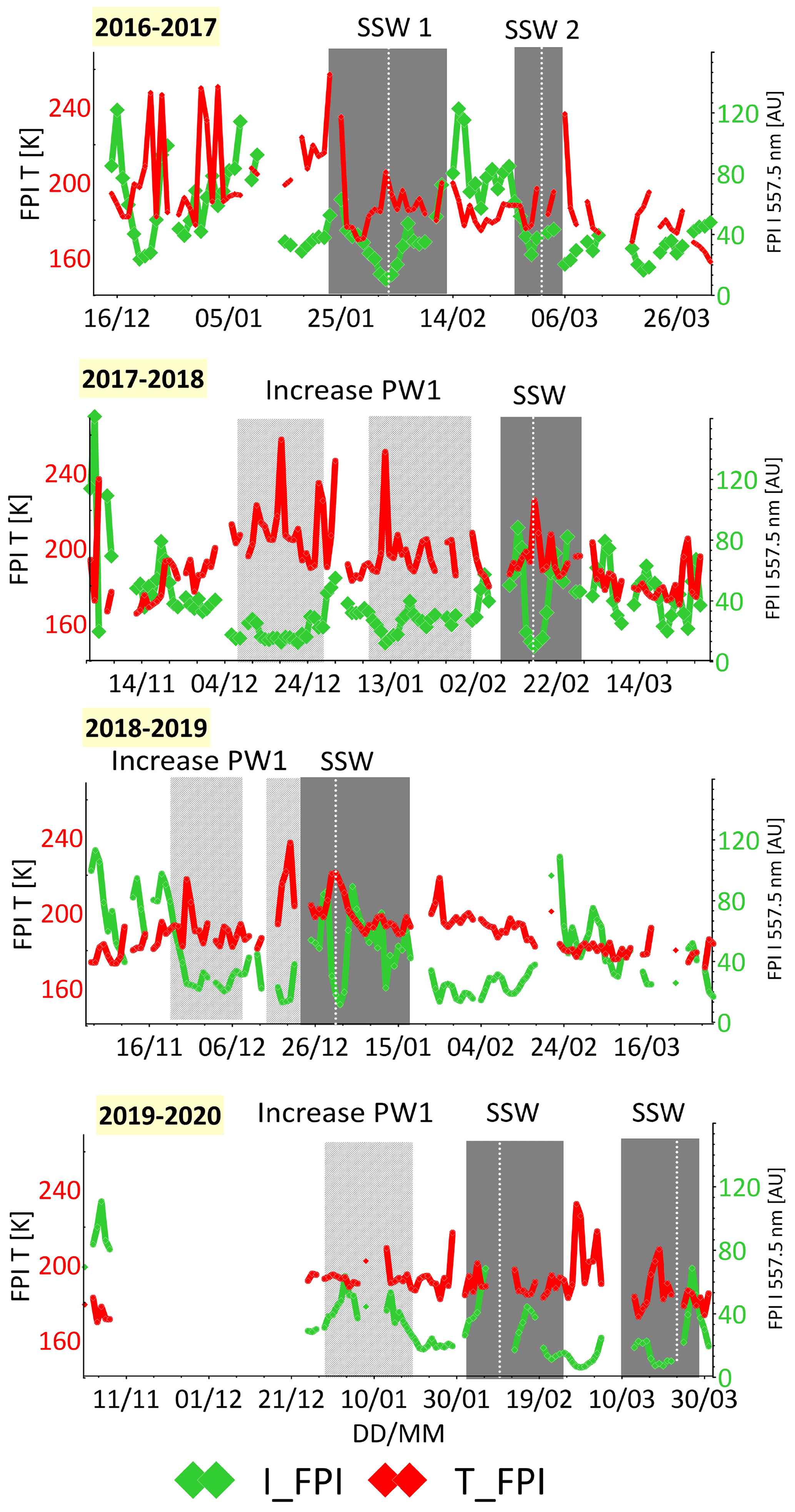
Figure 14 FPI-measured 557.7 nm emission (green line), temperature (red line), the PW1 amplitude increase period (light grey rectangle), the SSW periods (grey rectangle), and the day of the SSW maximal temperature (dotted white vertical line).

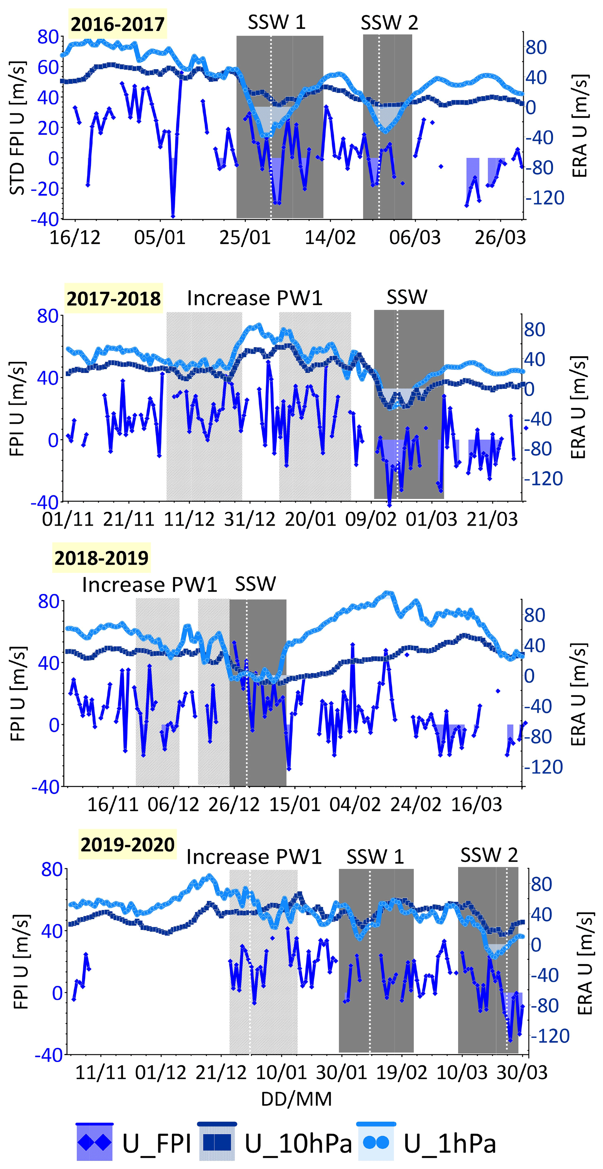
Figure 15 FPI-measured 557.7 nm zonal wind (blue line), zonal mean zonal wind by ERA 5 at 10 hPa (dark blue line) and at 1 hPa (light blue line), the PW1 amplitude increase period (light grey rectangle), the SSW periods (grey rectangle), and the day of the SSW maximal temperature (dotted white vertical line).

3.3 Spectral analysis through the Lomb–Scargle method

Researchers have also focused on diurnal variabilities of atmospheric characteristics during SSW impact (Merzlyakov et al., 2020; Pokhotelov et al., 2018; Manson et al., 2002). They report the tide variability due to non-linear interactions with the planetary waves. The Lomb–Scargle (LS) periodogram method is an appropriate technique for spectral analysis of the unequally sampled time series (Lomb, 1976; Scargle, 1982), especially for the FPI, because of gaps due to daylight, intense moonlight nights, and cloud cover. Figure 16a presents the calculated LS periodograms for the zonal wind variations observed during the 2017–2018 winter. The main spectral components with 24, 12, and 8 h periods dominate in the upper atmosphere. That is, these spectral components are present in the spectral characteristic for the zonal wind data. Twelve-hour oscillations have the largest amplitude. To check the validity of the retrieved spectral data, we prepared a testing sample of the data on the regular non-interrupted grid with 8, 12, and 24 h spectral components having the 0.3, 1, and 0.3 amplitudes, respectively. The sample time step was 15 min, which corresponds to the FPI data minimal time step. We also added the normal noise to the data with zero mean and sigma equal to 3. Figure 16c presents the LS periodogram for the artificial data sample. Figure 16b contains the LS periodogram of the described artificial data sample but with the same gaps (daytime, moonlight, clouds) of the observed zonal wind during the 2017–2018 winter. One can see a significant distortion in the spectral picture apparently due to the regular (daytime) 12 h gaps that significantly increase the initial 8 and 24 h spectral components and also generate additional spectral components. Therefore, a detailed spectral analysis for such non-regular data such as the FPI samples is apparently impossible without additional information, some special processing of the initial datasets, or significant modification of the analysis method. Still, we can estimate the diurnal variability of all tides by calculating the standard deviation of the diurnal dataset.

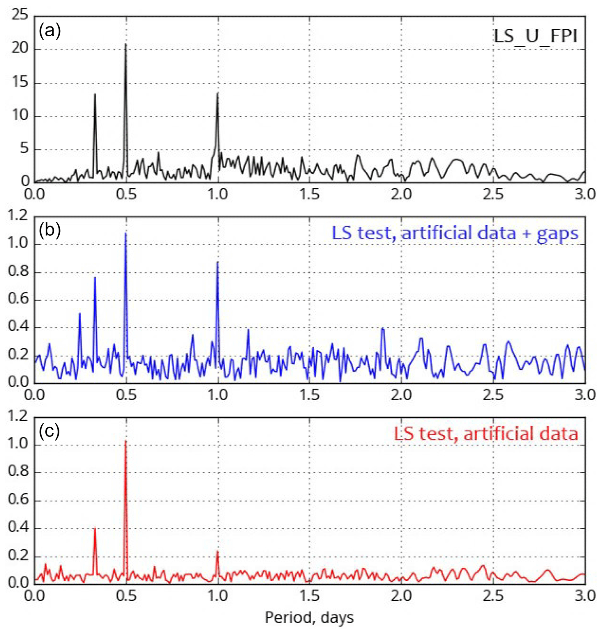
Figure 16 LS periodogram. (a) LS for the zonal wind variations observed during the 2017–2018 winter. (b) LS of the described artificial data sample but with the same gaps (daytime, moonlight, clouds) of the observed zonal wind during the 2017–2018 winter. (c) LS for the artificial data sample.

3.4 Standard deviations of the FPI-measured 557.7 nm emission and temperature

In this section, we analyse the standard deviation of the 557.7 nm emission, temperature, and zonal wind measurements for each night. During warmings and increased activity of planetary waves, emission fluctuations decrease, but temperature fluctuations increase during night. Figure 17 shows that temperature variations reach tens of degrees. Airglow and its night variations in the MLT were minimal during the periods of active stratosphere. Figures 14 and 17 show that variations in the mean values for the emission and temperature correlate directly with the behaviour of their standard deviations during the entire winter. This correlation is especially clear during PWs and SSWs.

Figure 17 FPI-measured standard deviation of the 557.7 nm emission (green line), the temperature (red line), the period of the PW1 amplitude increase (light grey rectangle), the SSW periods (grey rectangle), and the day of the SSW maximal temperature (dotted white vertical line).

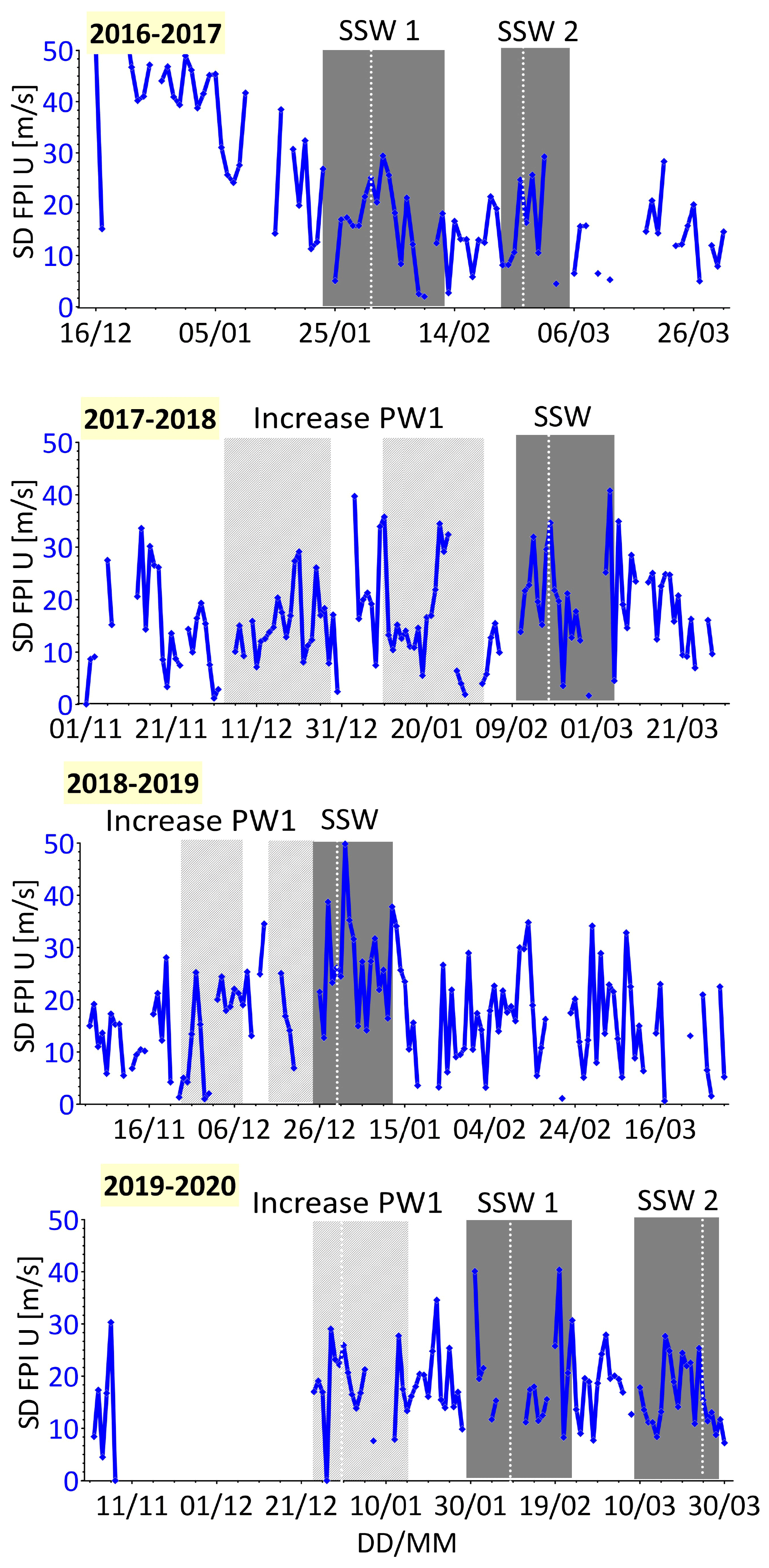
Figure 18 FPI-measured standard deviation of zonal wind, the period of the PW1 amplitude increase (light grey rectangle), the SSW periods (grey rectangle), and the day of the SSW maximal temperature (dotted white vertical line).

Unfortunately, in the 2019–2020 winter, there were technical problems with the interferometer measurements. Therefore, some of the data are missing for that winter. However, during the 2019–2020 winter, we also see the opposite behaviour of the mean values of temperature and emission and their standard deviations. The only peculiarity of that winter is that a sharp temperature increase occurred several days before the SSW onset. While we cannot determine why this occurred, it is possible that the influence was exerted by the stratosphere dynamics at 1 hPa, because there were higher temperatures throughout March at that height. In our opinion, the increase in temperature standard deviations is due to an increase in the MLT tidal amplitude, because the tides are the dominant mode in the MLT dynamics. It is possible that the height of the airglow layer 557.7 nm in the atmosphere changes during the SSWs and PWs. The lower part of the emission layer near the mesopause can be depleted, while a part of the emission layer above the mesopause remains unchanged or increases slightly due to the strong inverse temperature dependence of the reaction rate of the Barth mechanism. Thus, the FPI observes a decrease in the integral intensity of airglow and a corresponding increase in the tidal temperature as well as the nightly temperature during the active stratosphere. A possible reason for the observed effect is the depletion of atomic oxygen for the formation of the O (1^∘ S) state by the Barth mechanism near the mesopause due to vertical air movements.

The variations in the wind standard deviation appear to be noisier than those in the temperature standard deviation. Most often, we see that, during SSWs and PWs, the zonal wind standard deviation increases. However, this increase does not exceed the average background of wind variations even in the quiet stratosphere.

4 Conclusions

We studied the behaviour of the upper atmosphere during three winter seasons. We analysed the mean values of wind and temperature and their standard deviations during SSWs and PWs in the stratosphere. Due to the night-only nature of optical observations, we could not calculate tidal modes but characterized the tides by the standard deviation of each night-time period. The MLT response at the TOR appeared not to depend on the SSW location. The MLT responds equally, regardless of the SSW evolution over North America (2017–2018) or over the Asia–Pacific region (other winters). The 557.7 nm emission and its night variations decreased during SSWs and PW activations.

The temperature and its variations rise sharply and significantly during the active stratosphere. Note that the response of the emission intensity and temperature is the same during the periods of PW-increased amplitude and during SSW events (sometimes, during active PWs, it is even more significant). We speculate that, during SSWs and PWs, a change in the height profile of the green emission layer in the atmosphere is possible. The lower part of the emission layer intensity near the mesopause may deplete, whereas the part of the emission layer over the mesopause persists unchanged or insignificantly increases due to a strong reverse temperature dependence of the Barth mechanism reaction rate. Therefore, the FPI observes dimming of the integral emission intensity and corresponding increase in the tidal temperature variation and the temperature itself during these events. A possible reason for the observed effect is in the depletion of atomic oxygen for forming the O (1^∘ S) state in the Barth mechanism near the mesopause due to vertical air motion.

The response in the zonal wind is noticeable only during major SSWs. With a major SSW, the zonal wind reverses at MLT altitudes. The MLT wind inversion is observed during the wind inversion in the stratosphere; the height at which this occurs does not matter. The zonal wind at the MLT heights does not respond to the dynamics of planetary waves. The zonal wind night fluctuations show no significant dependence on SSW/PW activity. A possible reason may be weaker height gradients of the tidal amplitudes for the zonal wind as compared with the temperature or more significant noise due to the data gaps. Hence, we cannot draw convincing conclusions about the tidal response of the wind during SSWs in this study.