the Creative Commons Attribution 4.0 License.
the Creative Commons Attribution 4.0 License.
 | 23 Feb 2021
Distribution of Earth's radiation belts' protons over the drift frequency of particles
Using data on the proton fluxes of the Earth's radiation belts (ERBs) with energy ranging from 0.2 to 100 MeV on the drift L shells ranging from 1 to 8, the quasi-stationary distributions over the drift frequency fd of protons around the Earth are constructed. For this purpose, direct measurements of proton fluxes of the ERBs during the period from 1961 to 2017 near the geomagnetic equator were employed. The main physical processes in the ERB manifested more clearly in these distributions, and for protons with fd>0.5 mHz at L>3, their distributions in the {fd,L} space have a more regular shape than in the {E,L} space. It has also been found that the quantity of the ERB protons with fd ∼ 1–10 mHz at L∼2 does not decrease, as it does for protons with E > 10–20 MeV (with fd>10 mHz), but increases with an increase in solar activity. This means that the balance of radial transport and loss of ERB low-energy protons at L∼2 is disrupted in favor of transport of these protons: the effect of an increase in the radial diffusion rates with increasing solar activity overpowers the effect of an increase in the density of the dissipative medium.
- Article
(260 KB) - Full-text XML
- BibTeX
- EndNote


The Earth's radiation belts (ERBs) mainly consist of charged particles with energy from E∼100 keV to several hundreds of megaelectronvolts (MeV). In the field of the geomagnetic trap, each particle of the ERBs with energy E and equatorial pitch angle α0 (α is the angle between the local vector of the magnetic field and the vector of a particle velocity) makes three periodic movements: Larmor rotation, oscillations along the magnetic field line, and drift around the Earth (Alfvén and Fälthammar, 1963; Northrop, 1963).
Three adiabatic invariants (μ, K, Φ) correspond to these periodic motions of trapped particles as well as three periods of time or three frequencies: a cyclotron frequency (fc), a frequency of particle oscillations along the magnetic field line (fb), and a drift frequency of particles around the Earth (fd). For the near-equatorial ERB protons, we have fc ∼ 1–500 Hz, fb ∼ 0.02–2 Hz, and fd ∼ 0.1–20 mHz. The frequency fc increases by tens to hundreds of times with the distance of the particle from the plane of the geomagnetic equator (in proportion to the local induction of the magnetic field), and the frequency fb decreases by almost 2 times with increasing amplitude of particle oscillation.
The number of particles with a given frequency fc decreases rapidly with an increase in L and refers to higher and higher geomagnetic latitudes. For each given frequency fb, particles become more and more energetic with an increase in L (E∞L2), and their number becomes smaller.
Compared with the frequencies fc and fb, the drift frequency fd for one particle species has a much narrower range of values; it does not depend on the mass of the particles, and it very weakly depends on the amplitude of their oscillations (∼20 % variation). In this case, there are a significant number of particles corresponding to a certain value of fd on each L shell.
Therefore, it can be expected that the distributions of the ERB particles in the {fd,L} space will have a more regular shape than in the {E,L} space, and the main physical processes in these belts will manifest themselves more clearly in these distributions. Furthermore, it can also be expected that more fine features, which would not appear in the {E,L} space, can be revealed on this more ordered background.
Despite the importance of the drift frequency fd for the mechanisms of the ERB formation, reliable and sufficiently complete distributions of particles in the ERBs (over the frequency fd) have not been presented nor analyzed; indeed, this is the first time.
The analysis presented in this paper is limited to the protons of the ERB during magnetically quiet periods of observations (Kp < 2), when the proton fluxes and their spatial-energy distributions were quasi-stationary. In the following sections, the distributions of the ERB protons over their drift frequency fd are constructed from experimental data (Sect. 2) and analyzed (Sect. 3). The main conclusions of this work are given in Sect. 4.
The problem of methodical differences in measurements of the fluxes of protons of the radiation belts on different satellites was one of the main issues in this work. From the available published experimental data, those that are in good agreement with one another were selected, and all unreliable measurement results (with admixture of electrons and various ionic components of the ERB to the protons) were excluded from consideration. The reliable experimental results for proton fluxes and their anisotropy near the equatorial plane were then represent in the {E,L} space; this space is very efficient with respect to organizing experimental data obtained in different ranges of E and L.
In such a representation of experimental data, there is no need for interpolation and extrapolation of fluxes on the energy (in other representations, such necessity arises due to differences in channel widths and their positions on the energy scale for instruments installed on different satellites). In addition, with such a representation – the data from various experiments, in one figure – it is possible to construct the isolines of fluxes (and anisotropy of fluxes); these isolines cannot intersect with each other and, thus, allow for the exclusion of data that sharply fall out of the general picture (for more details, see Kovtyukh, 2020).
2.1 Spatial-energy distributions of the ERB protons near the equatorial plane
To construct the distributions of the ERB particles over the drift frequency, it is necessary to have reliable distributions of the differential fluxes of the ERB protons in the {E,L} space, where E is the kinetic energy of protons, and L is the drift shell parameter.
From the data of averaged satellite measurements of the differential fluxes of protons with an equatorial pitch angle α0≈90∘, the aforementioned distributions are constructed in Kovtyukh (2020) during quiet periods (Kp < 2) near the solar activity maximum in the 20th (1968–1971), 22th (1990–1991), 23th (2000), and 24th (2012–2017) solar cycles. Such distributions, separately for minima and maxima of the 11-year solar activity cycles, are also constructed from satellite data for other ionic components of the ERB (near the equatorial plane), but the most reliable and detailed picture was obtained for protons (see Kovtyukh, 2020).
In Fig. 1, one of these distributions is reproduced for periods near solar maxima (on the data from 1968 to 2017); here, data from different satellites are associated with different symbols. The numbers on the curves (isolines) refer to the values of the decimal logarithms of the differential fluxes J (cm2 s sr MeV)−1 of protons (with equatorial pitch angle α0≈90∘). The red lines correspond to the dependences fd (mHz) = (MeV) for the drift frequency of the near-equatorial protons in the dipole approximation of the geomagnetic field.
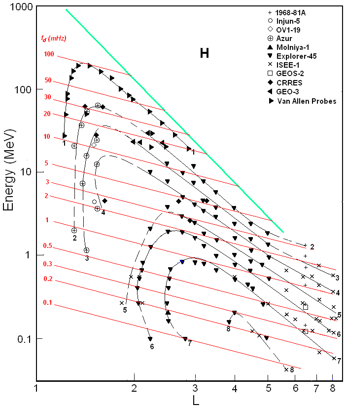
Figure 1Distribution of the differential fluxes J in the {E,L} space for protons with α0≈90∘ near maxima of the solar activity (from Kovtyukh, 2020). Data from satellites are associated with different symbols. The numbers on the curves refer to the values of the decimal logarithms of J. Fluxes are given in units of (cm2 s sr MeV)−1. The red lines correspond to the drift frequency fd (mHz), and the green line corresponds to the maximum energy of the trapped protons.
During the quiet periods considered in this work, the geomagnetic field at L<5 is close to the dipole configuration and (see Roederer and Lejosne, 2018). At large L, the magnetic field differs from the dipole configuration, even in quiet periods; this leads to the flattening of the isolines of the proton fluxes at L>5 in Fig. 1.
Only protons with energies less than some maximum values determined by the Alfvén criterion can be trapped on the drift shells. The Alfvén criterion is calculated as follows: , where ρc is the gyroradius of protons, and ρB is the radius of the curvature of the magnetic field (near the equatorial plane). According to this criterion and to the theory of stochastic motion of particles, the geomagnetic trap in the dipolar region can only capture and durably hold protons with E (MeV) < (Ilyin et al., 1984). The green line in Fig. 1 represents this boundary.
The distribution of the ERB proton fluxes, shown in Fig. 1, refers to the years of the solar maximum, but the solar-cyclic variations in the ERB proton fluxes are small and localized at L<2.5 (see Kovtyukh, 2020).
2.2 Spatial-energy distributions of the ERB protons outside the equatorial plane
The quasi-stationary fluxes J of the ERB particles with given energy and local pitch angle α usually decrease when the point of observation is shifted from the equatorial plane to higher latitudes along a certain magnetic field line. In the inner regions of the ERB, on L<5, angular distributions of protons usually have a maximum at the local pitch angle α=90∘. In the wide interval near this maximum, these distributions are well-described by the function (Parker, 1957), where A is the index of an anisotropy of a fluxes, B is the induction of a magnetic field at the point of measurements of these fluxes, and B0 is the induction of a magnetic field at the equatorial plane on the same magnetic line.
The empirical model of an anisotropy A(E,L) for the proton fluxes with E ∼ 0.1–2 MeV on L ∼ 2–5 near the equatorial plane for the quasi-stationary ERB (for quiet periods with Kp < 2) is presented in Fig. 2. The anisotropy index A of these fluxes is shown in Fig. 2, in the {E,L} space, in the form of isolines with the same values of A from 1.5 to 8.0 and with a step ΔA=0.5. The integer values of this index are plotted on the corresponding isolines as red numbers.
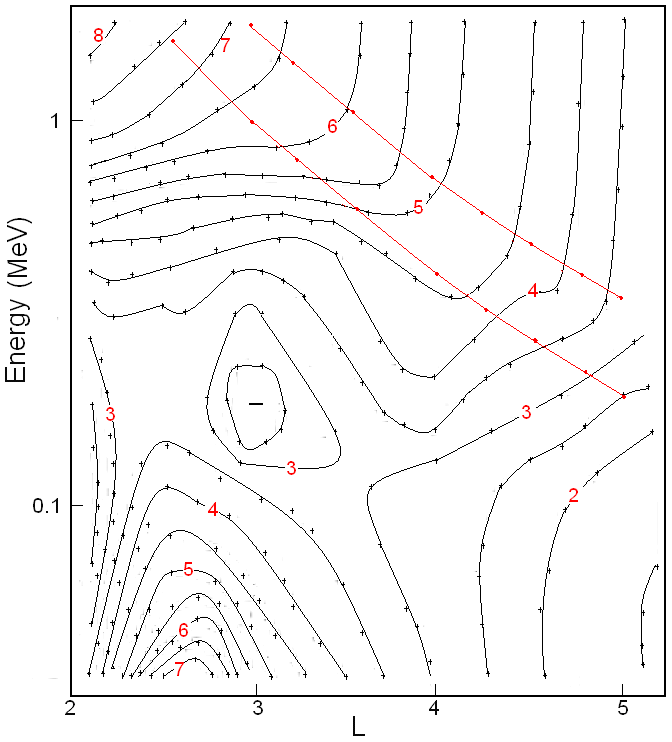
Figure 2Empirical model of the anisotropy index A(E,L) of the ERB proton fluxes averaged on the data from the satellites obtained near the plane of the geomagnetic equator. Values of A are given on isolines of the anisotropy: A = 1.5–8.5 with the step ΔA=0.5.
When constructing this model, we consider and analyze the data from the following satellites: Explorer 12 (Hoffman and Bracken, 1965), Explorer 14 (Davis, 1965), Explorer 26 (Søraas and Davis, 1968), OV1-14 and OV1-19 (Fennell et al., 1974), Explorer 45 (Williams and Lyons, 1974; Fritz and Spjeldvik, 1981; Garcia and Spjeldvik, 1985), ISEE-1 (Garcia and Spjeldvik, 1985; Williams and Frank, 1984), Van Allen Probes (Shi et al., 2016), and other satellites. These data were obtained from 1961 to 2015.
Figure 2 shows that the anisotropy of a proton flux monotonically increases with decreasing L (from A∼3.5 to A∼8.0) for rather high energy (>1 MeV). For E>0.3 MeV on L<3, anisotropy monotonically increases with increasing energy, but for E>0.5 MeV on L>3, it is almost energy independent.
Some small irregularities of the isolines in Fig. 2 are due to the fact that the experimental data used to construct this figure were obtained in different years, with different instruments, and during different solar activity intensities. At the same time, Fig. 2 demonstrates the important regularities of the pitch angle distributions of the quasi-stationary ERB proton fluxes.
In the {E>0.5 MeV, L>3} region, the isolines of the anisotropy index are almost parallel to each other and to the energy axis. This adiabatic regularity refers to protons belonging to the power-law tail of their energy spectra, the exponent of which practically does not change when L changes (at L>3). In Fig. 2, the red lines correspond to the lower boundary of the power-law tail of the ERB protons' energy spectra: MeV (see Kovtyukh, 2001, 2020).
The pattern of A(E,L) in the region on L>3 at E ∼ 0.2–0.5 MeV and the local minimum at L∼3 (E∼0.2 MeV) are connected with the local maximum in the quasi-stationary proton energy spectra of the ERB, which corresponds to MeV (see Kovtyukh, 2001, 2020).
These regularities in the pattern of A(E,L) are explained within the framework of the theory of radial transport (diffusion) of the ERB protons with conservation of the adiabatic invariants μ and K of their periodic motions (these issues were most fully considered in Kovtyukh, 1993).
Both the local maximum at L∼2.5 (E<0.1 MeV) and the region of low anisotropy at L∼2 (E∼0.1 MeV) in Fig. 2 are related to the ionization losses of protons.
With respect to the data from the satellites, the pitch angle distributions of the ERB proton fluxes strongly depend on magnetic local time (MLT) at L>5: the average index A values on the dayside are larger than on the nightside, and this dependence becomes more distinct with increasing energy (see, e.g., Shi et al., 2016). These results indicate that drift shells splitting (Roederer, 1970) play an important role in the formation of these distributions at L>5.
In the calculations performed here, it was assumed that the pitch angle distributions of the ERB proton fluxes at L>6, averaged over MLT, at α0∼90∘ are nearly isotropic near the equatorial plane.
High anisotropy for the fluxes of protons at E = 5–50 MeV and a strong dependence A(L) at the inner boundary of the inner belt (L = 1.15–1.40, = 1.0–1.7) were obtained on the DIAL satellite (Fischer et al., 1977). According to these data, there is an anisotropy index increase from A∼12 at L=1.25 to A∼60 at L=1.15, but this value is not dependent on L at L = 1.25–1.40. These results are supported by the data from the Resurs-01 N4 satellite for protons with E = 12–15 MeV, which were obtained at h∼800 km (Leonov et al., 2005). These data will be taken into account in our calculations.
The experimental results on the pitch angle distributions of the ERB proton fluxes and their anisotropy indexes were discussed in detail in Kovtyukh (2018).
2.3 Drift frequency distributions of the ERB protons
Based on the results shown in Figs. 1 and 2, one can calculate the distributions of the ERB protons over the drift frequency fd. In these calculations, the dipole model of the geomagnetic field was used, according to which (see, e.g., Roederer, 1970) the point of the magnetic field line at a given L and a geomagnetic latitude λ is located from the center of the dipole at a distance
Here, RE is the Earth's radius, and the field induction at a given L changes with changing λ as follows:
where .
The fact that the drift frequency fd of the nonrelativistic particles essentially only depends on their kinetic energy E and on L was also taken into account. This value depends very slightly on the particle pitch angle: with an increase in the geomagnetic latitude of the mirror point of the particle trajectory from 0 to 10∘, it increases by only 1.5 %, and in the range from 0 to 20–30∘, it increases by 5.8 %–12.5 %.
The number of protons with energies from E to E+dE per unit volume n is equal to the differential flux of these particles J (falling per unit time per unit area of the detector per unit solid angle) divided by the velocity v of these particles: . For nonrelativistic protons with mass m, this velocity is (.
Thus, in the near-equatorial region, between L and L+dL and within geomagnetic latitudes from 0 to ±λ0, the total number of nonrelativistic protons with mirror points within this region and with energy from E to E+dE, drifting on a given L with frequency fd(L,E) around the Earth, is
where m is the rest mass of a proton, is the differential fluxes, and E(L,fd) is the protons' energy. The first integral takes into account that the magnetic flux in the layer between shells L and L+dL is conserved when latitude λ changes, i.e., .
As a result of integrating the last expression over α0 and replacing cos λ≡t, we obtain
When integrating over equatorial pitch angles α0, Liouville's theorem and the conservation of the first adiabatic invariant (μ) are taken into account: and , where .
With an increase in λ from 0 to λ0=30∘, the value of the function increases from 1 to 1.32, i.e., deviates from the average value (1.16) by only 16 %. Most parts of the ERB protons are concentrated at these latitudes. Therefore, when calculating the last integral, we will assume that .
Thus the following expression is obtained:
where
and
When calculating the values of ΔN, we assume that . Finally, for the indicated ERB region near the equatorial plane, we obtain
where J, the differential fluxes of protons with equatorial pitch angle α0≈90∘, is given in units of (cm2 s sr MeV)−1, and the energy of protons E is given in megaelectronvolts. The dependence F(A) is shown in Fig. 3.

Figure 3Dependence of the factor F(A) in Eq. (1) on the anisotropy index A of the proton fluxes.
For protons of the ERB, the radial profiles ΔN(L,fd) for fd=0.2, 0.3, 0.5, 1, 2, 3, 5, 10, 20, and 30 mHz, calculated using Eq. (1) and Figs. 1–3, are shown in Fig. 4, and the frequency spectra ΔN(fd,L) at L=2, 2.5, 3, 4, 5, and 6 are shown in Fig. 5. Near each curve in Fig. 4, the corresponding value of fd (mHz) is indicated, and each spectrum in Fig. 5 shows the corresponding L value (these values are highlighted in red). In Figs. 4 and 5, for the sake of clarity, thin curves alternate with thick curves, and spectra at L=2 and 2.5 are highlighted in red in Fig. 5.
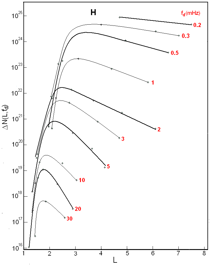
Figure 4Radial profiles ΔN(L,fd) for protons of the ERB with drift frequencies fd=0.2, 0.3, 0.5, 1, 2, 3, 5, 10, 20, and 30 mHz, plotted for periods of maximum solar activity. The fd values corresponding to each curve are highlighted in red. For clarity, thin curves are interspersed with thick curves.
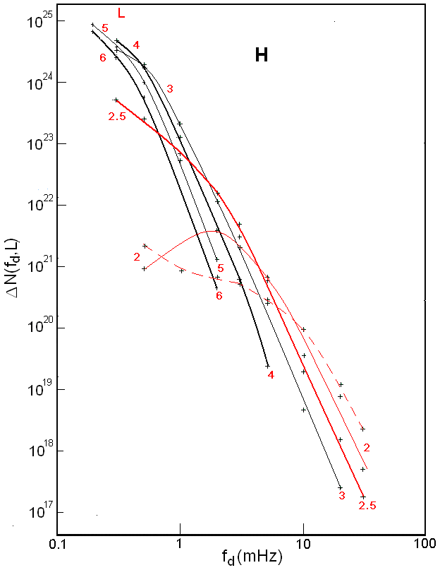
Figure 5Frequency spectra ΔN(fd,L) for protons of the ERB at L=2, 2.5, 3, 4, 5, and 6, plotted for periods of maximum solar activity. The values of L corresponding to each spectrum and spectra at L=2 and 2.5 are highlighted in red. The red dotted line shows the spectrum ΔN(fd,L) of the ERB protons at L=2, constructed from data during minimum periods of solar activity (see Kovtyukh, 2020). For clarity, thin curves are interspersed with thick curves.
The errors in these calculations mainly consist of the errors in the averaged experimental data shown in Figs. 1 and 2 (these errors are most significant at L<2) and the deviations of the geomagnetic field from the dipole model at L>5.
As λ0 decreases, the errors in our calculations will decrease. These errors can also be reduced by using numerical computer calculations. However, it should be taken into account that, even in very quiet periods of observations, the fluxes of the ERB protons, as well as the energy spectra and pitch angle distributions of these fluxes, may experience changes that exceed the errors in our calculations.
In agreement with the results of experimental and theoretical studies, at L>2, the main mechanism for the formation of the ERB protons is the radial diffusion of particles from the outer boundary of the geomagnetic trap to the Earth under conservation the adiabatic invariants μ and K (see, e.g., Lejosne and Kollmann, 2020; Kovtyukh, 2016, 2018).
Figures 1 and 2 make it possible to determine the regions of the {E,L} space near the equatorial plane in which the ionization losses of ions during their radial diffusion can be neglected and where they cannot.
The isolines of proton fluxes in Fig. 1 at sufficiently large E and L ascend with decreasing L, in the direction of increasing energy, in strict agreement with the adiabatic laws of the radial transport of particles. At lower L these isolines do change the direction of their course under the influence of ionization losses, which increase rapidly with decreasing L (see Kovtyukh, 2020, for details).
At sufficiently large values of E and L, isolines of the anisotropy index in Fig. 2 pass practically parallel to each other and parallel to the energy axis, in agreement with the laws of adiabatic transport of particles with power-law energy spectra (see Kovtyukh, 1993). At lower E and L, a more complex picture is formed under the influence of ionization losses (for more details, see Kovtyukh, 2001, 2018).
With decreasing L, the radial diffusion is decreased very rapidly, and the belt of protons with E > 10–20 MeV on L<2 is generated mainly as result of the decay of neutrons of albedo which are knocked from the atmospheric atoms' nuclei by the galactic cosmic ray's (GCR) protons. This mechanism (CRAND) is simulated in many contemporary studies based on experimental data (see, e.g., Selesnick et al., 2007, 2013, 2014, 2018).
The mechanisms of formation of the ERB under the action of radial diffusion and CRAND are manifested and clearly differ both in the radial profiles ΔN(L,fd) and in the frequency spectra ΔN(fd,L) of protons.
Let us consider the manifestations of these mechanisms in Figs. 4 and 5 as well as the related effects.
In contrast to the radial profiles of fluxes J(L,E), the radial profiles ΔN(L,fd) for protons with fd<5 mHz (see Fig. 4) have much less steep outer edges, and their steepness decreases with decreasing frequency fd. This effect is mainly connected with an increase in the volume of magnetic tubes (factor L3 in Eq. 1 from Sect. 2.3) and with a decrease in the anisotropy index of proton fluxes with increasing L.
At the same time, in comparison with the radial profiles J(L,E), the radial profiles ΔN(L,fd) have much steeper inner edges. This effect is mainly connected to the large anisotropy of proton fluxes in the corresponding region of {E,L} space and to the rapid growth of the anisotropy index with decreasing L in this region. It is especially expressed in the radial profiles ΔN(L,fd) at fd ∼ 0.3–1 mHz (see Fig. 4); this is due to the fact that the anisotropy index of proton fluxes strongly depends on E and L in the corresponding region of {E,L} space (see Fig. 2).
Radial profiles ΔN(L, fd) at fd>10 mHz are formed by the CRAND mechanism. They have a maximum at L ∼ 1.5–2.0, and the steepness of their inner and outer edges does not differ as much as for lower frequencies fd (see Fig. 4). When constructing these profiles, it was taken into account that an anisotropy index A of proton fluxes at E = 5–50 MeV does not depend on L at L = 1.25–1.40: (Fischer et al., 1977; Leonov et al., 2005).
The shape of the spectra ΔN(fd,L) at L>3 is determined, first of all, by the shape of the energy spectra of proton fluxes J(E,L) at the outer boundary of the geomagnetic trap. Gradually, as the particles diffuse to the Earth, their energy spectra are transformed under the action of betatron acceleration and ionization losses of particles.
In contrast to the energy spectra of proton fluxes J(E,L), distributions ΔN(fd,L) of the ERB protons over their drift frequency fd (Fig. 5) differ much less from each other at L>3. Such convergence of the spectra ΔN(fd,L) is driven by an increase in the volume of magnetic tubes and a decrease in the anisotropy index of the ERB proton fluxes with increasing L. Figure 5 demonstrates the closeness to the adiabatic transformations of the spectra ΔN(fd,L) when L changes at L>3.
The energy spectra of near-equatorial proton fluxes J(E,L) with MeV at L>3 in quiet periods have a local maximum at MeV and a power-law tail (, where ) at MeV (Kovtyukh, 2001, 2018, 2020).
The frequency spectra of the ERB protons at L>3 weakly depend on L and over a wide range of fd have a close to power-law shape with an exponent (at , where mHz at L ∼ 3–6, ∼2 mHz at L=2.5 and ∼5 mHz at L=2). Note that the spread of the parameter γ for the frequency spectra of protons is almost 2 times less than for their energy spectra. These spectra become more rigid (flattened) at .
Thus, the average exponents of the power-law tail of the energy and frequency spectra of protons differ by Δγ=0.46, and there is no local maximum in the frequency spectra at fd>2 mHz at L>2.5. The main role in such differences in the shape of the energy and frequency spectra of protons was played by the factor F(A) in Eq. (1), in which the anisotropy index A is a function of E and L (see Figs. 2 and 3). Note that in the {E>0.5 MeV, L>3} region the anisotropy index A, as well as the protons energy, is transformed according to adiabatic laws when L changes (see Fig. 2 and the related text).
These results confirm our hypothesis about the ordering of the distributions of protons over their drift frequency fd in the outer regions of the ERB, at L>3, where most of the ERB protons are located and where the radial diffusion of protons overpowers their ionization losses.
At all L, the frequency spectra ΔN(fd,L) become more flat at small fd (at small E) under the influence of ionization losses. However, in the range of high fd (from 3–5 to 30 mHz), for protons with high energies and low ionization losses, the protons frequency spectra even have a power-law tail at L=2 (see Fig. 5).
For protons with fd<0.5 mHz, which correspond to the ERB protons of the lowest energies, ionization losses lead to the same consequences at higher L shells: the radial profiles ΔN(L,fd) approach each other, and the spectra ΔN(fd,L) flatten out (see Figs. 4 and 5).
In the region of the steep inner edge of the radial distributions ΔN(L,fd), spectra ΔN(fd,L) of the ERB protons gradually become increasingly rigid with decreasing L and rapidly diverge from each other (see Figs. 4 and 5). In the range of small fd at L<2.5, the connection between these distributions and the shape of the boundary energy spectra of protons is gradually lost.
These results indicate a violation of the order in the distributions of protons under the influence of ionization losses.
In Fig. 5, the dotted line also shows the spectrum ΔN(fd,L) of the ERB protons at L=2, constructed from experimental data for periods of low solar activity between the 19th–20th, 20th–21th, 21th–22th, and 22th–23th solar cycles (see Fig. 1 in Kovtyukh, 2020). Figure 5 shows that there were more protons at the minimum of solar activity at L=2 for fd>10 mHz, whereas there were more protons at the maximum of solar activity for fd ∼ 1–10 mHz.
The effect of a decrease in the ΔN(fd, L) values for protons with fd>10 mHz at L<2 with an increase in solar activity is mainly connected with a decrease in the fluxes of protons with E > 10–20 MeV here. This effect is well-known; it is described by the CRAND mechanism (see, e.g., Selesnick et al., 2007) and was considered in detail in Kovtyukh (2020). With an increase in solar activity, the densities of atmospheric atoms and ionospheric plasma on small L shells significantly increase, which leads to an increase in ionization losses of the ERB protons, whereas the power of their main source (CRAND) practically does not change. As a result, the equilibrium fluxes and ΔN(fd,L) for protons with fd>10 mHz are established at lower levels.
However, the effect of an increase in ΔN(fd,L) for fd ∼ 1–10 mHz at low L with increasing solar activity, corresponding to the protons of lower energies, was discovered here for the first time.
With decreasing E (and fd) of protons, their ionization losses increase, and if the fluxes of low-energy protons in the inner belt were also formed by the CRAND mechanism, one would have observed an even stronger increase in their fluxes with decreasing solar activity compared with protons with E > 10–20 MeV (fd>10 mHz). However, for protons with fd ∼ 1–10 mHz, we see the opposite effect in the spectra ΔN(fd,L) at L=2 (Fig. 5), which is not described by the CRAND mechanism.
On the other hand, it was proved that quasi-stationary fluxes of protons with E<15 MeV at L∼2 are mainly formed by the mechanism of protons' radial diffusion from the external region of the ERB (Selesnick et al., 2007, 2013, 2014, 2018). These fluxes and ΔN(fd,L) values for fd ∼ 1–10 mHz at L=2 are formed as a result of a balance of the competing processes of radial diffusion of protons and their ionization losses.
The rates of transport of the ERB protons to the Earth (radial diffusion) rapidly increase with decreasing particles energy (see Kovtyukh, 2016). In addition, with an increase in solar activity, the average level of geomagnetic fluctuations in the ERB increases. Under the influence of these factors, one can expect a significant increase in the intensity of radial diffusion of the low-energy protons at low L with an increase in solar activity. As a result, the effect of the increasing density of a dissipative medium with an increase in solar activity is overpowered by the more significant effect of the increasing rates of radial diffusion of protons.
According to numerous experimental data, a wide variety of complex spectra of powerful pulsations of magnetic and electric fields in the considered ultra-low frequency (ULF) range, which are non-regularly distributed over L, can be generated in the geomagnetic trap during magnetic storms; these pulsations can lead to local acceleration and losses of the ERB particles (see, e.g., Sauvaud et al., 2013). Such effects will violate the regular characteristics of the proton distributions shown in Figs. 4 and 5. However, during quiet periods (Kp < 2), the amplitudes of such pulsations are small and lead only to the radial diffusion of particles.
From the data on near-equatorial ERB proton fluxes (with energy from 0.2 to 100 MeV and drift L shells ranging from 1 to 8), their quasi-stationary distributions over the drift frequency of particles around the Earth (fd) were constructed. The results of calculations of the number ΔN of the ERB protons within 30∘ of geomagnetic latitude at different L and fd for periods of maximum solar activity are presented. They differ from the corresponding distributions of the ERB protons for periods of low solar activity only at L<2.5 (for comparison, the spectra of these distributions are given at L=2).
The radial profiles of these distributions ΔN(L,fd) have only one maximum that shifts toward the Earth with increasing fd. In comparison to the proton fluxes' profiles J(L,E), the radial profiles ΔN(L,fd) at fd<5 mHz have steeper inner edges and flatter outer edges. However, the radial profiles ΔN(L,fd) at fd>10 mHz, which are formed by the CRAND mechanism, have inner and outer edges with only a slightly difference from each other with respect to the steepness of their profiles.
In contrast to the energy spectra of proton fluxes J(E,L), the frequency spectra ΔN(fd, L) of the ERB protons at L>3 are weakly dependent on L, and for sufficiently large fd they have a nearly power-law shape with an exponent . There is no local maximum in these spectra in the region, as in the corresponding J(E,L) spectra.
The main physical processes in the ERB (radial diffusion, ionization losses of particles, and the CRAND mechanism) manifested clearly in these distributions.
Distributions ΔN(L,fd) and ΔN(fd,L) of the ERB protons in the region have a more regular shape than in the corresponding region of the {E,L} space. The majority of the ERB protons exist in this region, and their radial diffusion overpowers their ionization losses during the transport of particles to Earth.
In the region of the steep inner edges of the radial distributions ΔN(L,fd), the spectra ΔN(fd,L) of protons rapidly diverge from each other with decreasing L, and these spectra become flattened at low frequencies. These results indicate a violation of the order in these distributions of protons under the influence of ionization losses.
With increasing solar activity, the number of protons ΔN(fd,L) at L∼2 decreases for fd>10 mHz and increases for fd ∼ 1–10 mHz. The effect at high fd, corresponding to protons with E>15 MeV, is well-known and is described in the framework of the CRAND mechanism.
However, the opposite effect at low fd, corresponding to the lower-energy protons, is discovered here for the first time. This effect can be associated with the fact that the low-frequency part of the spectrum ΔN(fd,L) of protons, even at L∼2, is mainly formed by the mechanism of proton transport from the outer regions of the ERB. This effect may indicate that the average rates of radial diffusion of protons also increase with increasing solar activity. For low-energy protons at L∼2, the effect of increasing density of a dissipative medium with increasing solar activity is overpowered by the increase in the rates of radial diffusion of particles.
Comparing this result with the results for ions with Z≥2 at L>2.5 (see Kovtyukh, 2020), one can conclude that the amplitude of solar-cyclic variations of the radial diffusion coefficient DLL increases with decreasing E and L (Z is the charge of the atomic nucleus with respect to the charge of the proton).
All data from this investigation are presented in Figs. 1–5.
The author declares that there is no conflict of interest.
The author is very grateful to the reviewers for their important and fruitful comments and proposals regarding the paper and to topical editor, Elias Roussos, for editing this paper.
This paper was edited by Elias Roussos and reviewed by two anonymous referees.
Alfvén, H. and Fälthammar, C.-G.: Cosmical Electrodynamics, Fundamental Principles, Clarendon Press, Oxford, UK, 1963.
Davis, L. R.: Low energy trapped protons and electrons, in: Proceedings of the Plasma Space Science Symposium, Washington, D. C., USA, 11–14 June 1963, Astrophysics and Space Sience Library, Vol. 3, edited by: Chang, C. C. and Huang, S. S., Reidel, Dordrecht, the Netherlands, 212–226, 1965.
Fennell, J. F., Blake, J. B., and Paulikas, G. A.: Geomagnetically trapped alpha particles, 3. Low-altitude outer zone alpha-proton comparisons, J. Geophys. Res., 79, 521–528, https://doi.org/10.1029/JA079i004p00521, 1974.
Fischer, H. M., Auschrat, V. W., and Wibberenz, G.: Angular distribution and energy spectra of protons of energy MeV at the lower edge of the radiation belt in equatorial latitudes, J. Geophys. Res., 82, 537–547, https://doi.org/10.1029/JA082i004p00537, 1977.
Fritz, T. A. and Spjeldvik, W. N.: Steady-state observations of geomagnetically trapped energetic heavy ions and their implications for theory, Planet. Space Sci., 29, 1169–1193, https://doi.org/10.1016/0032-0633(81)90123-9, 1981.
Garcia, H. A. and Spjeldvik, W. N.: Anisotropy characteristics of geomagnetically trapped ions, J. Geophys. Res., 90, 359–369, https://doi.org/10.1029/JA090iA01p00359, 1985.
Hoffman, R. A. and Bracken, P. A.: Magnetic effects of the quiet-time proton belt, J. Geophys. Res., 70, 3541–3556, https://doi.org/10.1029/JZ070i015p03541, 1965.
Ilyin, B. D., Kuznetsov, S. N., Panasyuk, M. I., and Sosnovets, E. N.: Non-adiabatic effects and boundary of the trapped protons in the Earth's radiation belts, B. Russ. Acad. Sci. Phys., 48, 2200–2203, 1984.
Kovtyukh, A. S.: Relation between the pitch-angle and energy distributions of ions in the Earth's radiation belts, Geomagn. Aeron., 33, 453–460, 1993.
Kovtyukh, A. S.: Geocorona of hot plasma, Cosmic Res., 39, 527–558, https://doi.org/10.1023/A:1013074126604, 2001.
Kovtyukh, A. S.: Deduction of the rates of radial diffusion of protons from the structure of the Earth's radiation belts, Ann. Geophys., 34, 1085–1098, https://doi.org/10.5194/angeo-34-1085-2016, 2016.
Kovtyukh, A. S.: Ion Composition of the Earth's Radiation Belts in the Range from 100 keV to 100 MeV/nucleon: Fifty Years of Research, Space Sci. Rev., 214, 1–30, https://doi.org/10.1007/s11214-018-0560-z, 2018.
Kovtyukh, A. S.: Earth's radiation belts' ions: patterns of the spatial-energy structure and its solar-cyclic variations, Ann. Geophys., 38, 137–147, https://doi.org/10.5194/angeo-38-137-2020, 2020.
Lejosne, S. and Kollmann, P.: Radiation Belt Radial Diffusion at Earth and Beyond, Space Sci. Rev., 216, 1–78, https://doi.org/10.1007/s11214-020-0642-6, 2020.
Leonov, A., Cyamukungu, M., Cabrera, J., Leleux, P., Lemaire, J., Gregorie, G., Benck, S., Mikhailov, V., Bakaldin, A., Galper, A., Koldashov, S., Voronov, S., Casolino, M., De Pascale, M., Picozza, P., Sparvolli, R., and Ricci, M.: Pitch angle distribution of trapped energetic protons and helium isotope nuclei measured along the Resurs-01 No. 4 LEO satellite, Ann. Geophys., 23, 2983–2987, https://doi.org/10.5194/angeo-23-2983-2005, 2005.
Northrop, T. G.: The Adiabatic Motion of Charged Particles, Wiley-Interscience, New York, USA, 1963.
Parker, E. N.: Newtonian development of the dynamical properties of ionized gases of low density, Phys. Rev., 107, 924–933, https://doi.org/10.1103/PhysRev.107.924, 1957.
Roederer, J. G.: Dynamics of Geomagnetically Trapped Radiation, Springer, New York, USA, https://doi.org/10.1007/978-3-642-49300-3, 1970.
Roederer, J. G. and Lejosne, S.: Coordinates for representing radiation belt particle flux, J. Geophys. Res.-Space, 123, 1381–1387, https://doi.org/10.1002/2017JA025053, 2018.
Sauvaud, J.-A., Walt, M., Delcourt, D., Benoist, C., Penou, E., Chen, Y., and Russell, C. T.: Inner radiation belt particle acceleration and energy structuring by drift resonance with ULF waves during geomagnetic storms, J. Geophys. Res.-Space, 118, 1723–1736, https://https://doi.org/10.1002/jgra.50125, 2013.
Selesnick, R. S., Looper, M. D., and Mewaldt, R. A.: A theoretical model of the inner proton radiation belt, Space Weather, 5, S04003, https://doi.org/10.1029/2006SW000275, 2007.
Selesnick, R. S., Hudson, M. K., and Kress, B. T.: Direct observation of the CRAND proton radiation belt source, J. Geophys. Res.-Space, 118, 7532–7537, https://doi.org/10.1002/2013JA019338, 2013.
Selesnick, R. S., Baker, D. N., Jaynes, A. N., Li, X., Kanekal, S. G., Hudson, M. K., and Kress, B. T.: Observations of the inner radiation belt: CRAND and trapped solar protons, J. Geophys. Res.-Space, 119, 6541–6552, https://doi.org/10.1002/2014JA020188, 2014.
Selesnick, R. S., Baker, D. N., Kanekal, S. G., Hoxie, V. C., and Li, X.: Modeling the proton radiation belt with Van Allen Probes Relativistic Electron-Proton Telescope data, J. Geophys. Res.-Space, 123, 685–697, https://doi.org/10.1002/2017JA024661, 2018.
Shi, R., Summers, D., Ni, B., Manweiler, J. W., Mitchell, D. G., and Lanzerotti, L. J.: A statistical study of proton pitch-angle distributions measured by the Radiation Belt Storm Probes Ion Composition Experiment, J. Geophys. Res.-Space, 121, 5233–5249, https://doi.org/10.1002/2015JA022140, 2016.
Søraas, F. and Davis, L. R.: Temporal variations of 100 keV to 1700 keV trapped protons observed on satellite Explorer 26 during first half of 1965, Report X-612-68-328, NASA Goddard Space Flight Center, Greenbelt, MD, USA, 48 pp., 1968.
Williams, D. J. and Lyons, L. R.: The proton ring current and its interaction with plasmapause: Storm recovery phase, J. Geophys. Res., 79, 4195–4207, https://doi.org/10.1029/JA079i028p04195, 1974.
Williams, D. J. and Frank, L. A.: Intense low-energy ion populations at low equatorial altitude, J. Geophys. Res., 89, 3903–3911, https://doi.org/10.1029/JA089iA06p03903, 1984.