Seasonal evolution of winds, atmospheric tides, and Reynolds stress components in the Southern Hemisphere mesosphere–lower thermosphere in 2019

In this study we explore the seasonal variability of the mean winds and diurnal and semidiurnal tidal amplitude and phases, as well as the Reynolds stress components during 2019, utilizing meteor radars at six Southern Hemisphere locations ranging from midlatitudes to polar latitudes. These include Tierra del Fuego, King Edward Point on South Georgia island, King Sejong Station, Rothera, Davis, and McMurdo stations. The year 2019 was exceptional in the Southern Hemisphere, due to the occurrence of a rare minor stratospheric warming in September. Our results show a substantial longitudinal and latitudinal seasonal variability of mean winds and tides, pointing towards a wobbling and asymmetric polar vortex. Furthermore, the derived momentum fluxes and wind variances, utilizing a recently developed algorithm, reveal a characteristic seasonal pattern at each location included in this study. The longitudinal and latitudinal variability of vertical flux of zonal and meridional momentum is discussed in the context of polar vortex asymmetry, spatial and temporal variability, and the longitude and latitude dependence of the vertical propagation conditions of gravity waves. The horizontal momentum fluxes exhibit a rather consistent seasonal structure between the stations, while the wind variances indicate a clear seasonal behavior and altitude dependence, showing the largest values at higher altitudes during the hemispheric winter and two variance minima during the equinoxes. Also the hemispheric summer mesopause and the zonal wind reversal can be identified in the wind variances.

1 Introduction

Gravity waves (GWs) originating at the lower atmosphere by a number of sources are an essential driver of the mesosphere–lower thermosphere (MLT) dynamics, forcing a meridional flow due to a zonal drag, which drives the mesopause temperature up to 100 K away from the radiative equilibrium (e.g., Lindzen, 1981; Becker, 2012), introducing a residual circulation from the cold summer to the warm winter pole. This important coupling mechanism is caused by GWs carrying energy and momentum from their source regions to the altitude of their breaking, coupling different vertical layers in the atmosphere (Fritts and Alexander, 2003; Ern et al., 2011; Geller et al., 2013). The primary forcing of the MLT at small scales is by gravity waves arising from various tropospheric sources, among them flow over orography (mountain waves), deep convection (convective gravity waves), frontal systems, and jet stream imbalances and shear instabilities (Fritts and Nastrom, 1992; see also the review by Fritts and Alexander, 2003, and Plougonven and Zhang, 2014). These various GWs typically have horizontal phase speeds comparable to the mean winds at higher altitudes; hence they are strongly influenced by varying winds along their plane of propagation. GWs can propagate upward until they become dynamical unstable or they are filtered by critical levels, where they undergo breaking and dissipation, resulting in local mean flow accelerations that act as sources of non-primary GWs.

GW breaking dynamics occurs on relatively small horizontal scales, 10–100 km, whereas non-primary GW dynamics occurs at larger scales, 100–300 km, and arises due to the local, transient mean-flow accelerations accompanying GW momentum transport (Dong et al., 2020; Fritts et al., 2020). Non-primary GWs at larger scales also arise due to interactions among larger-scale GWs in global models unable to resolve GW breaking dynamics (Becker and Vadas, 2018; Vadas and Fritts, 2001; Vadas and Becker, 2018). Importantly, however, non-primary GWs accompanying GW breaking and interactions at lower altitudes require propagation over large depths to become significant; hence, they play more significant roles in the lower thermosphere.

Although GWs are such an important driver of the MLT, the number of observations is rather sparse. Very often the GW activity is inferred by subtracting a background from the wind or temperature observations to estimate potential GW energy or wind variations (Ehard et al., 2015; Baumgarten et al., 2017; Chu et al., 2018; Rüfenacht et al., 2018; Stober et al., 2018b; Wilhelm et al., 2019). Satellite observations provide an estimate of absolute momentum fluxes from the troposphere up to the mesosphere and most importantly a global coverage (Ern et al., 2011; Trinh et al., 2018; Hocke et al., 2019). However, satellite observations are lacking the directional information, and, thus, there is some ambiguity about the forcing or whether the GW momentum flux is accelerating or decelerating the mean flow.

Vincent and Fritts (1987) introduced, over 2 decades ago, a radar technique to determine the vertical flux of zonal and meridional momentum utilizing medium-frequency (MF) radars using two pairs of co-planar beams. This technique was also applied by Placke et al. (2015a, b) to determine momentum fluxes above Andenes in northern Norway. However, there are only a few MF radars worldwide that are able to conduct such measurements. Furthermore, at altitudes above 94 km, MF radars tend to underestimate the wind speeds, which might lead to some systematic bias in the derived momentum flux (Wilhelm et al., 2017). Hocking (2005) presented a method to obtain the Reynolds stress tensor components from meteor radar observations. Based on this, several studies applied the method to optimize the data analysis as it appeared to be challenging to get the technique implemented (Placke et al., 2011a, b; Andrioli et al., 2013). Fritts et al. (2010b) and Fritts et al. (2012b) presented a momentum flux meteor radar design to overcome some of the difficulties and evaluated the momentum flux observations using synthetic data (Fritts et al., 2010a), which finally provided evidence that these systems can be used to measure momentum fluxes reliably. This led to several studies using these new-generation systems (de Wit et al., 2014, 2016, 2017; Spargo et al., 2019; Vierinen et al., 2019) or more powerful radars such as MU radars (Riggin et al., 2016).

Climatologies of mean winds and tides are also rather sparse at the Southern Hemisphere (SH) and are essentially affected by the vertical coupling of upward propagating gravity waves but also provide a temporal and spatially variable background for the gravity wave propagation itself. Recent studies with general circulation models (GCMs) have shown that mean winds are essential to understand the GW forcing (Liu, 2019; Shibuya and Sato, 2019). This is also the case for tides, which provide essentially temporal variable critical filtering for the vertical propagation of the GWs (Heale et al., 2020). In the past there were several studies about mesospheric winds or tides, which were often limited to a single station or investigated only a certain tidal or wave component (Batista et al., 2004; Fritts et al., 2010b, 2012b) and for tides (Beldon and Mitchell, 2010; Conte et al., 2017). Recently, Liu et al. (2020) used several meteor radars at the Southern Hemisphere to systematically investigate the 8 and 6 h tides and to obtain a more comprehensive picture of the latitudinal and longitudinal characteristics of these tidal modes. Furthermore, meteor radar observations have turned out to provide a valuable and independent method to validate general circulation models with data assimilation (McCormack et al., 2017) or to investigate the inter-day variability of tidal amplitudes and phases (Stober et al., 2020).

In this study, we present a cross-comparison of mean winds and the diurnal and semidiurnal tide for six southern hemispheric meteor radars located at midlatitudes and polar latitudes. We present observations from 2019 and investigate the latitudinal and longitudinal differences of these meteorological parameters at each radar site to provide a comprehensive overview and systematic analysis of the wind and tidal and gravity wave dynamics by applying a unified diagnostic. The meteor radars are located at Tierra del Fuego (TDF), King Edward Point (KEP) on South Georgia island (Jackson et al., 2018), King Sejong Station (KSS) on King George Island (Lee et al., 2018, 2016), and Rothera (ROT) Station (Sandford et al., 2010) located on the Antarctic Peninsula, as well as Davis Antarctic Station (DAV) (Holdsworth et al., 2004) and McMurdo (McM) Antarctic Station. We discuss the presented results within the context of the stratospheric polar vortex for the year 2019. For this purpose, we complement our meteor radar observations with data from the Microwave Limb Sounder (MLS) on board the AURA satellite (Livesey et al., 2006; Schwartz et al., 2008). Furthermore, we utilize a recently developed retrieval algorithm, which builds on the initial momentum flux analysis formulation reported by Hocking (2005). In particular, we introduce a generalized approach to obtain wind variances and momentum fluxes from several meteor radars (many of which are standard low power systems) for the year 2019, which evolved into one of the rare minor stratospheric warming events during September (Yamazaki et al., 2020). We briefly summarize how the Reynolds stress components, also called momentum fluxes and wind variances, are derived from a Reynolds decomposition. The Reynolds decomposition is achieved by utilizing an adaptive spectral filter (ASF), which allows the decomposition of the meteor radar wind time series into mean winds, tidal components, and a GW residual (Stober et al., 2017; Baumgarten and Stober, 2019; Stober et al., 2020), similar to the S transform used in previous studies (Stockwell et al., 1996; Fritts et al., 2010a).

The paper is structured as follows: in Sect. 2 we present a brief introduction to the wind retrievals, the derivation of the Reynolds stress components, and the implemented momentum flux and GW retrieval. Section 3 contains the results of the mean flow terms, which are mean winds, diurnal and semidiurnal tides, and their seasonal behavior, as well as the determined momentum fluxes and wind variances. Our results are discussed in Sect. 4, and the conclusions are provided in Sect. 5.

2 Observations and methods

2.1 Meteor radar observations

In this study, we use observations obtained with six meteor radars operating in the SH between 53 and 79^∘ S in latitude. Four of the meteor radars can be grouped into a cluster around the Drake Passage consisting of the Southern Argentina Agile Meteor Radar (SAAMER) at Rio Grande, Tierra del Fuego, Argentina (hereafter referred to as TDF), King Sejong Station on King George Island (KSS), Rothera (ROT) on the Antarctic Peninsula, and King Edward Point (KEP) on South Georgia island. The other two radars are located almost opposite the Drake Passage at McMurdo (McM) and Davis Antarctic stations (DAV). Figure 1 shows two panels with stereographic projections of the SH, where the radar locations are represented by red dots (left panel and Table 1). The right panel in this figure shows a color contour map of the mean elevations around each radar system to identify potential orographic wave forcing sources underneath the observation volumes.

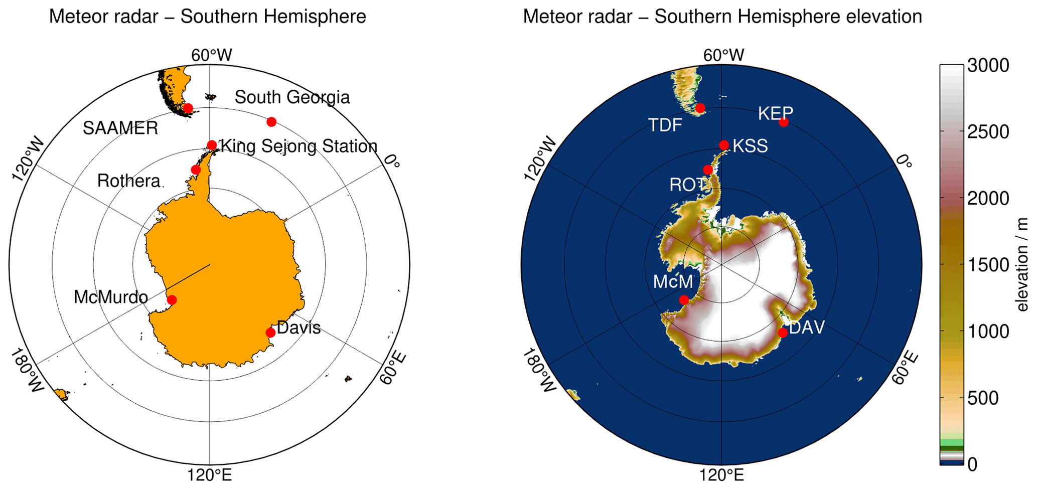
Figure 1 Stereographic projection of the geographic location of the meteor radars used in this study and a map of the terrain elevation of Antarctica, the Antarctic Peninsula, and southern Argentina to visualize the orography around each radar station. The maps are generated using etopo1 data (Amante and Eakins, 2009).

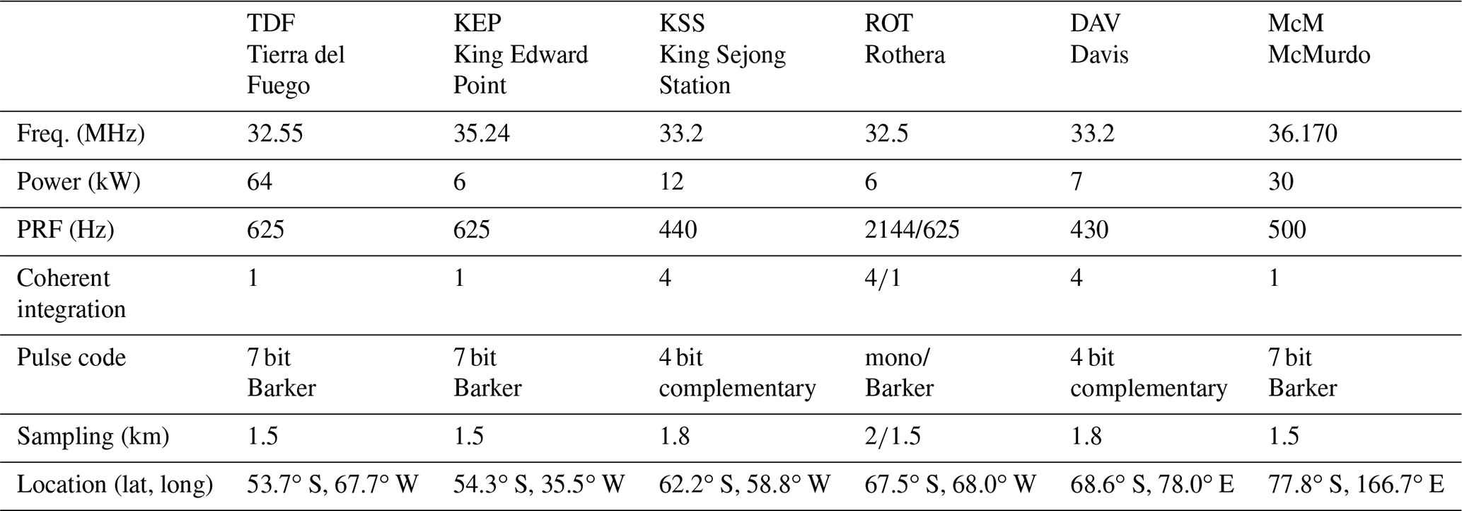
A technical summary of the radars is provided in Table 1. Most of the systems have been in operation for more than a decade and have provided reliable and continuous observations. Although most of these systems have been operated without major parameter changes, both ROT and TDF meteor radars have been upgraded during the observing period of our study. Until February 2019, the ROT system used a high pulse repetition frequency (PRF) meteor mode, with a PRF of 2144 Hz, a 2 km range sampling, and four coherent integrations. After this time, the system was upgraded and resumed operation transmitting a 7 bit Barker code with 1.5 km range sampling and a PRF of 625 Hz. We also noted a significant noise or interference at ROT before the upgrade in January/February that did not allow trustworthy momentum fluxes to be derived. Further, we also restricted our analysis of mean winds and tides to the altitude range between 80–100 km. In addition, in September 2019, the TDF transmitting scheme also changed. The original design of the TDF transmitter (TX) configuration used eight three-element crossed Yagi antennae arranged in a circle of diameter 27.6 m, each transmitting in opposite phasing of every other Yagi (Janches et al., 2014). In 2019, the system transmission strategy was upgraded with the deployment of a single new TX antenna, with the goal of improving the detection rate of meteors at larger zenith angles for astronomical purposes (Janches et al., 2020). By concentrating the full power of TDF in one TX antenna, a more uniform detection pattern is achieved that satisfies this original requirement but also increases the number of events detected at larger zenith angles. Finally, the McM radar is the most recent installation, which, although it is not the most powerful radar, provides a very good altitude coverage. This is partly explained by the sporadic meteor sources and the southern location of the McM meteor radar. The helion, antihelion, and the south apex meteor source are above the local horizon all the time, contributing to the observed sporadic meteor fluxes at McM and yielding a much weaker seasonality in the altitude variation of the meteor layer (Janches et al., 2004). In addition, meteors arriving from these sources enter the atmosphere at fairly low entry angles (<20^∘; see Schult et al., 2017 for a Northern Hemisphere radar), leading to a much smoother ablation profile of the meteoroids, and, hence, the released meteoric material is spread over a larger segment of the meteor flight path, increasing the detectability. On the other side, the orbit geometry alone does not yet provide a sufficient explanation for the better altitude coverage at McMurdo; however, a more detailed investigation is beyond the scope of the paper.

Table 1 Technical parameters of the meteor radars.

Several of the meteor radars used in this study employ the standard meteor radar configuration of an array of five Yagi antennas for reception, with a spacing of 2 and 2.5λ (Jacobs and Ralston, 1981; Jones et al., 1998). McM was set up in a different configuration with 1.5 and 2λ spacing due to topographic constraints. Similar to other meteor radars, most of them use a single Yagi antenna for transmission. Only TDF employed a beam forming transmission scheme, resulting in eight main beams, as described earlier, but changed to the use of the single crossed Yagi antenna late during the period studied here (Janches et al., 2014, 2020). A more detailed description of the King Sejong Station meteor radar can be found in Lee et al. (2018) and for the DAV meteor radar in Holdsworth et al. (2004).

2.2 Retrieval of winds and momentum flux

Meteor radars have been used to measure winds in the mesosphere–lower thermosphere (MLT) for several decades. Typically winds are obtained by least-squares fits, solving for the horizontal wind velocities after binning the data into altitude and time intervals (Hocking et al., 2001; Holdsworth et al., 2004). In this study we retrieve winds using the algorithm presented in Stober et al. (2018a), which includes the treatment of the geometry of the full Earth, based on the WGS84 rotation ellipsoid to provide more precise altitude estimates and geodetic coordinates for each meteor, a spatiotemporal Laplace filter, and a nonlinear error propagation, which is described in more detail in Gudadze et al. (2019). The wind retrievals are cross-validated against NAVGEM-HA (McCormack et al., 2017; Stober et al., 2020). The results presented in this paper are based on winds with a temporal resolution of 1 h and a vertical resolution of 2 km. The minimum number of meteors per time and altitude bin for a successful fit is four.

For the case of momentum fluxes, Hocking (2005) proposed a method using typical meteor radars, which was later echoed and reformulated as correlations by Vierinen et al. (2019). In this work, we present a brief derivation of the Reynolds stress tensor and show how the different tensor elements are estimated from the meteor radar observations. The starting point is the well-known radial wind equation. Each meteor will form a trail that will be detected by the radar and will drift with the background wind. The radar will then detect that radial velocity, via Doppler shift in the received signal, and the three components of the background wind can be calculated for each detected meteor using the mathematical convention (reference to east and counterclockwise rotation):

$$\begin{array}{}\text{(1)}& v_{\mathrm{rad}}=u\cdot \cos \left(\mathit{\varphi }\right)\sin \left(\mathit{\theta }\right)+v\cdot \sin \left(\mathit{\varphi }\right)\sin \left(\mathit{\theta }\right)+w\cdot \cos \left(\mathit{\theta }\right),\end{array}$$

where u, v, and w are the three wind components (zonal, meridional, and vertical, respectively), ϕ is the azimuth angle, θ is the off-zenith angle, and v_rad is the observed radial wind velocity. Further, it is straightforward to use the standard Reynolds decomposition of the wind, separating the wind components into a mean flow ($\stackrel{\mathrm{‾}}{u},\stackrel{\mathrm{‾}}{v},\stackrel{\mathrm{‾}}{w}$) and wind fluctuations (u^′, v^′, w^′):

$$\begin{array}{}\text{(2)}& \begin{array}{rlr}u& =& \stackrel{\mathrm{‾}}{u}+u^{\prime }\\ v& =& \stackrel{\mathrm{‾}}{v}+v^{\prime }\\ w& =& \stackrel{\mathrm{‾}}{w}+w^{\prime }.\end{array}\end{array}$$

As we are mainly interested in the momentum flux associated with GWs, the mean flow terms containing the background wind and the diurnal and semidiurnal tide have to be subtracted/removed from the observed radial velocities for each meteor. Thus, we model the mean flow radial velocity by

$$\begin{array}{}\text{(3)}& \stackrel{\mathrm{‾}}{v_{\mathrm{radm}}}=\stackrel{\mathrm{‾}}{u}\cdot \cos \left(\mathit{\varphi }\right)\sin \left(\mathit{\theta }\right)+\stackrel{\mathrm{‾}}{v}\cdot \sin \left(\mathit{\varphi }\right)\sin \left(\mathit{\theta }\right)+\stackrel{\mathrm{‾}}{w}\cdot \cos \left(\mathit{\theta }\right).\end{array}$$

The radial velocity fluctuations ($v_{\mathrm{rad}}^{\prime }$), which now only contain GW contributions, are obtained by subtracting the mean flow radial velocity ($\stackrel{\mathrm{‾}}{v_{\mathrm{radm}}}$) from the observed radial velocity (v_rad) measurements:

$$\begin{array}{}\text{(4)}& v_{\mathrm{rad}}^{\prime }=v_{\mathrm{rad}}-\stackrel{\mathrm{‾}}{v_{\mathrm{radm}}}.\end{array}$$

Furthermore, the GW fluctuations can be modeled by

$$\begin{array}{}\text{(5)}& v_{\mathrm{radm}}^{\prime }=u^{\prime }\cdot \cos \left(\mathit{\varphi }\right)\sin \left(\mathit{\theta }\right)+v^{\prime }\cdot \sin \left(\mathit{\varphi }\right)\sin \left(\mathit{\theta }\right)+w^{\prime }\cdot \cos \left(\mathit{\theta }\right).\end{array}$$

Considering that these radial velocity fluctuations are mostly driven by GW, the Reynolds stresses can be computed by minimizing the following quantity (Hocking, 2005):

$$\begin{array}{}\text{(6)}& \mathrm{\Lambda }=\sum ({\left(v_{\mathrm{rad}}^{\prime }\right)}^{\mathrm{2}}-{\left(v_{\mathrm{radm}}^{\prime }\right)}^{\mathrm{2}}{)}^{\mathrm{2}}.\end{array}$$

Inserting Eq. (5) into Eq. (6) leads to the well-know momentum flux terms:

$$\begin{array}{}\text{(7)}& \begin{array}{rl}\mathrm{\Lambda }& =\sum ({\left(v_{\mathrm{rad}}^{\prime }\right)}^{\mathrm{2}}-({u^{\prime }}^{\mathrm{2}}\cdot \cos \left(\mathit{\varphi }{)}^{\mathrm{2}}\sin \right(\mathit{\theta }{)}^{\mathrm{2}}\\ & +{v^{\prime }}^{\mathrm{2}}\cdot \sin \left(\mathit{\varphi }{)}^{\mathrm{2}}\sin \right(\mathit{\theta }{)}^{\mathrm{2}}+{w^{\prime }}^{\mathrm{2}}\cdot \cos (\mathit{\theta }{)}^{\mathrm{2}}\\ & +\mathrm{2}{u}^{\prime }{v}^{\prime }\cdot \cos \left(\mathit{\varphi }\right)\sin \left(\mathit{\varphi }\right)\sin (\mathit{\theta }{)}^{\mathrm{2}}\\ & +\mathrm{2}{u}^{\prime }{w}^{\prime }\cdot \cos \left(\mathit{\varphi }\right)\sin \left(\mathit{\theta }\right)\cos \left(\mathit{\theta }\right)\\ & +\mathrm{2}{v}^{\prime }{w}^{\prime }\cdot \sin \left(\mathit{\varphi }\right)\sin \left(\mathit{\theta }\right)\cos \left(\mathit{\theta }\right)){)}^{\mathrm{2}}.\end{array}\end{array}$$

Solving Eq. (7) for the unknown Reynolds stress components is straightforward. Typically, the terms $u^{\prime }{w}^{\prime }$, $v^{\prime }{w}^{\prime }$, and $u^{\prime }{v}^{\prime }$ are also called momentum fluxes, and the symmetric Reynolds stress tensor is given by

$$\begin{array}{}\text{(8)}& {\mathit{\tau }}_{ij}^{\prime }=\mathit{\rho }\stackrel{\mathrm{‾}}{u_i{u}_j}=\mathit{\rho }\cdot \left[\begin{array}{ccc}{u^{\prime }}^{\mathrm{2}}& u^{\prime }{v}^{\prime }& u^{\prime }{w}^{\prime }\\ u^{\prime }{v}^{\prime }& {v^{\prime }}^{\mathrm{2}}& v^{\prime }{w}^{\prime }\\ u^{\prime }{w}^{\prime }& v^{\prime }{w}^{\prime }& {w^{\prime }}^{\mathrm{2}}\end{array}\right],\end{array}$$

where ρ is the atmospheric density at the altitude of the measurement, and the other terms in the tensor denote the Reynolds stress components (wind variances and momentum fluxes), which have units of squared velocity fluctuations. The Reynolds stress components are derived from the RANS (Reynolds-averaged Navier–Stokes) equations, assuming an incompressible Newtonian fluid and that the Reynolds average of the fluctuations vanishes ($\stackrel{\mathrm{‾}}{u^{\prime }}=\mathrm{0}$), which requires the averaging to be long enough to cover the inertia GW periods of several hours or longer. The spatial scales can theoretically be estimated by selecting different volumes inside the domain area; however, practically the meteor statistics is often not sufficient to get reliable results.

However, there are some caveats of the theory outlined above, when it comes to implementing the algorithm and actually applying it to meteor radar observations. One difficulty is the Reynolds decomposition into the mean flow and the GW fluctuations. Previous studies often limited the analysis to a narrower angular region (Fritts et al., 2010a; Placke et al., 2015a) using only off-zenith angles between 10–50^∘, reducing significantly the number of meteors for the analysis per time and altitude bin, which in turn required longer averaging or was achieved by an active beam forming antenna. Such an antenna directed more energy towards an angular region as for TDF (Fritts et al., 2010b, a) or the meteor radar at Trondheim (de Wit et al., 2014). The process by which this much stricter angular selection of meteors improved the momentum flux estimates was the reduction of projection errors due to the Earth's ellipsoid shape, which caused apparent and arbitrary contributions to the fluctuation terms. Stober et al. (2018a) proposed to minimize this type of uncertainty by computing each meteor's geodetic position relative to the WGS84 reference ellipsoid, which improves the altitude determination but also reduces projection errors for the azimuth and off-zenith angle. The benefit of this full Earth geometry correction is that there is no longer a need to reduce the angular region, and all meteors up to off-zenith angles of 65^∘ can be used for the analysis. Typical specular meteor radars (single Yagi antenna on transmission) detect most meteors at off-zenith angles between 50 and 70^∘. However, meteors at larger zenith angles are further away from the radar and, thus, are more prone to altitude errors. The typical angular precision of the employed receiver arrays is approximately 1.5–1.7^∘ (Jones et al., 1998). A limit of 65^∘ presents a more optimal choice to maximize the number of meteors entering the analysis while keeping a sufficient altitude precision.

Another important aspect related to the momentum flux estimation is the proper removal of the background flow, which was already outlined by Fritts et al. (2010a), Placke et al. (2011b), and Andrioli et al. (2013) and later confirmed by de Wit et al. (2014). In particular, tides have large amplitudes in the MLT, causing large vertical and temporal shears within a time and altitude bin. Noting that Hocking (2005) and Placke et al. (2011b) suggested the use of at least 30 meteors for a successful momentum flux fit, which is often achieved by temporal averaging, the importance of the temporal shear becomes evident.

In this study we use the adaptive spectral filter (ASF) to perform the Reynolds decomposition to characterize the background flow and the GW fluctuations. A first version of the ASF(1D) (temporal domain) was presented in Stober et al. (2017). Here we make use of the ASF(2D), which employs a vertical regularization constraint for the mean wind and tides, assuming a smooth vertical phase progression for each wave without an explicit vertical wavelength threshold (Pokhotelov et al., 2018; Baumgarten and Stober, 2019; Wilhelm et al., 2019). The ASF accounts for the continuous variation of the mean flow as well as for the intermittent behavior of the tides. Thus, we obtain hourly resolved background wind fields for each altitude and time bin for the zonal, meridional, and vertical wind component, respectively. This background wind field contains the mean flow and the diurnal, semidiurnal, and terdiurnal tidal component. However, the terdiurnal tide usually has a much smaller amplitude (Liu et al., 2020) compared to the diurnal and semidiurnal tides and, thus, is not discussed here further. Furthermore, we perform a linear interpolation of the background wind field to the actual occurrence time and altitude for each meteor to estimate the v_radm term, minimizing any contribution from the background flow. This procedure is effective in mitigating possible contamination due to tides and permits the use of a much longer averaging window. In this study we use 64 h and a minimum of 100 meteors to determine the Reynolds stress components. However, for the seasonal climatology, only solutions with more than 1000 meteors enter the statistics.

The algorithm is implemented similar to that performed for wind retrievals in Stober et al. (2018a). The first guess is provided by a classical least-squares fit. Based on this initial iteration, we compute the spatiotemporal Laplace filter, which provides a predictor for each time and altitude bin. This predictor enters all further iterations as regularization (Tikhonov) and is updated each time. The spatiotemporal Laplace filter turns out to be beneficial for ill-conditioned problems due to the random occurrence of meteor detections and asymmetries in the spatial sampling; these can result in difficulties in determining all parameters with similar quality.

Furthermore, we perform a nonlinear error propagation similar to the one presented in Gudadze et al. (2019). The statistical uncertainties are updated in each iteration step. We also tested barrier functions to penalize negative values of ${u^{\prime }}^{\mathrm{2}},{v^{\prime }}^{\mathrm{2}}$, and ${w^{\prime }}^{\mathrm{2}}$, respectively. Such negative values were reported in Placke et al. (2011a), but this appears to be a minor issue in our retrievals. Only a negligible number of fits resulted in negative values for just some of the radar systems utilized in this work.

In addition, we performed some test retrievals to account for the vertical velocity bias intrinsic to the meteor radar observations. Specular meteors have trail lengths of up to several kilometers where the radio waves are scattered, and, thus, meteors entering the Earth's atmosphere at steep entry angles can encounter strong vertical wind shears, which lead to a rotation of the trail, causing systematic errors. In particular, during the local summer months, this can lead to a systematic deviation of a few centimeters per second for midlatitude stations.

Very often wind fits are performed by assuming w=0 m s⁻¹ (Hocking et al., 2001; Holdsworth et al., 2004). However, here we use the retrievals as presented in Stober et al. (2018a), who used the vertical wind velocity as quality control. Typically, we obtain daily mean values of the order of ±0.25 m s⁻¹, which is more than an order of magnitude less than reported by Egito et al. (2016). However, the remaining bias due the vertical winds, which potentially has the wrong sign, had no impact on the retrieved Reynolds stresses.

Finally, in order to get confidence in the retrievals, we performed several test cases similar to the ones presented in Fritts et al. (2010a). Therefore, we extracted the observed meteor detections from TDF and synthesized wind fields including altitude-dependent mean winds and tides with a vertical wavelength of 80 km and various altitude-dependent GW fields to optimize the retrieval setting with respect to the regularization strength, the required statistics, and the applied averaging. Performing these tests, we find minor deviations from the synthetic wind and GW fields only at the upper and lower edges of the meteor layer. The tidal amplitudes were retrieved within ±2 m s⁻¹ compared to the synthetic data. The momentum fluxes agreed for the 30 d median remarkably well. We also tested the possibility to retrieve the vertical wind fluctuation amplitudes and found mean deviations of ±0.01 m s⁻¹ residual bias for the synthetic fields and about ±0.25 m s⁻¹ bias in our observations.

2.3 MLS satellite observations

To bring the local radar observations into the global context we calculate the geostrophic zonal wind as described in Matthias and Ern (2018) from geopotential height (GPH) data from the Microwave Limb Sounder (MLS) on board the Aura satellite (Waters et al., 2006; Livesey et al., 2015). MLS has a global coverage from 82^∘ S to 82^∘ N on each orbit and a usable height range from approximately 11 to 97 km (261–0.001 hPa), with a vertical resolution of ∼4 km in the stratosphere and ∼14 km at the mesopause. The temporal resolution is 1 d at each location, and data are available from August 2004 until the present (Livesey et al., 2015). Version 4 MLS data were used in this paper, along with the application of the most recent recommended quality screening procedures from Livesey et al. (2015). For our analyses the original orbital MLS data are accumulated in grid boxes with 10^∘ grid spacing in longitude and 5^∘ in latitude. Afterwards they are averaged at every grid box and for every day, generally resulting in a global grid with values at every grid point.

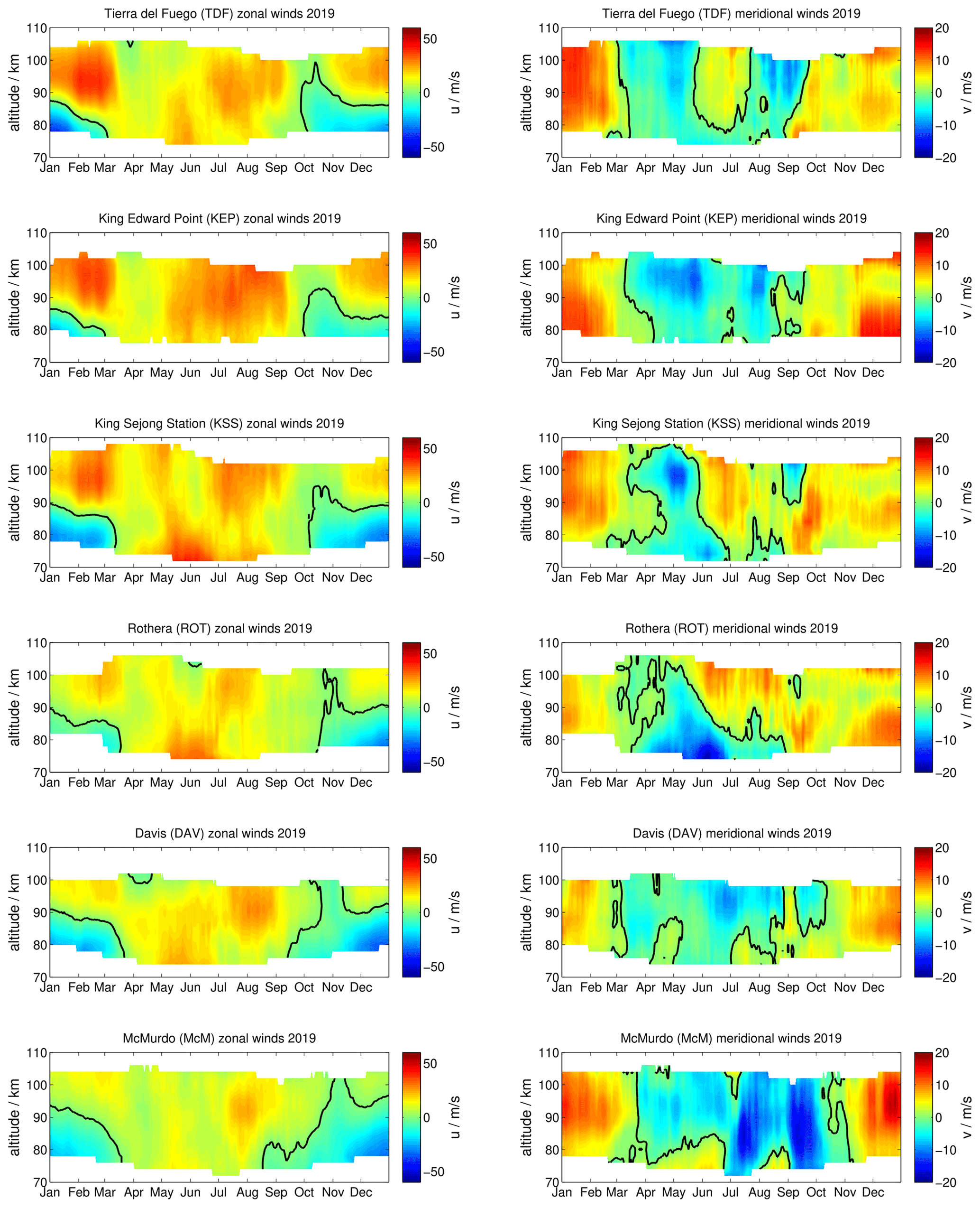
Figure 2 Comparison of zonal and meridional mean winds for each station during the year 2019. The left column shows the zonal component and the right column the meridional wind. All stations are sorted according to their latitude from TDF, KEP, KSS, ROT, and DAV to McM.

3 Results

3.1 Mean winds 2019

As pointed out in the previous section, we perform a Reynolds decomposition in order to separate a mean flow from the GW fluctuations. Thus, we analyze the data with the adaptive spectral filter (ASF) technique (Baumgarten and Stober, 2019) to obtain daily mean winds, as well as diurnal and semidiurnal tides.

We first compare the seasonal zonal and meridional winds of all six locations to identify any seasonal and local differences. Figure 2 shows the seasonal zonal and meridional wind pattern during 2019 obtained from the daily mean zonal and meridional winds after applying a 30 d running median shifted by 1 d. This reveals any seasonal variability by removing atmospheric waves with shorter periods. A similar analysis was applied in Wilhelm et al. (2019) for meteor radars in the Northern Hemisphere in order to derive mean wind climatologies. Significant differences between the locations can be observed from this figure, in particular during the SH winter seasons (JJA). Both TDF and KEP observations, operated at almost the same latitude at 54^∘ S, show a similar morphology for the zonal winds, and only the meridional winds deviate from each other during June and July. At the tip of South America, TDF shows that the meridional winds experience a sign reversal around June/July, which is not present over KEP. The meridional winds also seem to have a semiannual oscillation at both locations.

Further polewards at KSS and ROT (62 and 67^∘ S, respectively), which are at a similar longitude as TDF, the zonal winds reflect a similar seasonal behavior compared to KEP and TDF but with a slightly weaker wind magnitude. However, the meridional winds are fairly consistent during the summer months compared to the midlatitude radars but deviate considerably during the winter season. There is even a noticeable difference between KSS and ROT, even though the systems are located rather close together. At ROT and KSS the meridional winds only show a typical winter behavior during April, May, and June and approximately northward winds for the other months above 80–85 km. Only during September and at altitudes above 90 km above KSS does a short southward wind patch occur.

Comparing the observed wind fields measured at ROT and DAV, which are only separated by 2^∘ in latitude but by 170^∘ in longitude, further emphasizes the existence of a significant asymmetry in the southern hemispheric wind systems. As expected, looking at the general morphology, the seasonal zonal wind pattern for 2019 is remarkably similar between both locations. There are only marginal differences in the zonal magnitudes considering the overall agreement of the zonal wind structures. This is also the case for the meridional winds during the summer months (DJF). However, during the winter season, the meridional wind structure is significantly different between both stations. The morphology at DAV appears to be less asymmetric, with a tendency to show increased southward wind magnitudes towards the end of the winter season, whereas at ROT the highest southward winds are recorded at the begin of the winter season 2019.

The southernmost location in our analysis is McM at 78^∘ S. The seasonal zonal wind morphology compares well with that measured at DAV and ROT but shows much weaker wind magnitudes. Similar to observations in the Northern Hemisphere, the summer zonal wind reversal altitude also increases with increasing southern latitude. Compared to DAV, the meridional winds are intensified during the summer and winter seasons. Furthermore, the asymmetry during the winter months is also present at McM, which shows, similarly to DAV, the highest southward meridional winds towards the end of the winter season as a double structure. In fact, the southward meridional winds at McM during July and September 2019 are the strongest of all locations.

Figure 3 Same as Fig. 2 but for the diurnal tidal amplitudes.

Figure 4 Same as Fig. 2 but for the diurnal tidal phases.

3.2 Diurnal tidal amplitudes and phases measured during 2019

Atmospheric tides provide a time-variable background filter for the vertical propagation of GWs, which can, depending on the tidal phase and the propagation direction of the GW, lead to GW breaking and dissipation. These breaking events might trigger/foster the generation of secondary or non-primary waves (Heale et al., 2020). Thus, tides are essentially contributing to the Reynolds decomposition. In particular, the day-to-day variability is crucial for the momentum flux analysis. Typically, atmospheric tides are derived assuming phase stability over a certain period of time, which can be several days, weeks, or months (Murphy et al., 2006; Hoffmann et al., 2010; Conte et al., 2017; He et al., 2018; Pancheva et al., 2020). More recent studies favor much shorter windows of 24 to 48 h to account for the intermittent behavior of tides (Stober et al., 2017; Wu et al., 2019; de Araújo et al., 2020; Das et al., 2020), in particular, phases of atmospheric tides that appear not to be constant with time (Ward et al., 2010; Baumgarten and Stober, 2019; Stober et al., 2020). In this study, all tidal amplitudes and phases were determined with the ASF, which, similar to wavelet spectra, adapts the window length to the period of the fitted frequencies. The obtained daily tidal amplitudes are vector-averaged using 30 d medians centered at the respective day to derive the seasonal variation.

Figure 3 presents the seasonal variation of the diurnal tidal amplitudes measured at each station. Although the daily mean winds showed significant differences between TDF, KEP, KSS, and ROT, the seasonal behavior of the diurnal tide is rather consistent between all four locations. There is a pronounced summer maximum in the zonal and meridional amplitudes from January to February at altitudes from 78–106 km. The meridional tidal amplitudes tend to exceed the zonal amplitude by up to 10 m s⁻¹. At altitudes above 100 km the diurnal tide remained of significant magnitude until May 2019. Evidently, for the other months the diurnal tidal amplitudes remained fairly weak (<10 m s⁻¹) at altitudes between 80–100 km during 2019. KSS and ROT indicate a small diurnal tidal enhancement for July/August and in December below 80 km and above 100 km altitude. The December enhancements are also found at TDF but almost disappear at KEP. DAV measurements show basically the same seasonal diurnal tide behavior but with weaker amplitudes. The winter diurnal tidal enhancement in June/July appears to be more pronounced. However, the southernmost meteor radar at McM observes a significantly different seasonal diurnal tidal pattern. The summer maximum is much more pronounced compared to the other stations and shows amplitudes of 20 m s⁻¹ from January to April at 90 km and above and again from October to December. There is also a noticeable difference between the zonal and the meridional diurnal tidal amplitude. The zonal component indicates a winter minimum, whereas the meridional component shows a tidal enhancement.

Diurnal tidal phases are shown in Fig. 4. The tidal phases are given in UTC; hence, longitudinal differences are present as phase shifts. As expected the diurnal phases are much more variable during time with low tidal amplitudes for TDF, KEP, KSS, and ROT. During the summer months of January and February 2019, the diurnal phases are more stable and indicate rather long vertical wavelengths but with significant differences between the zonal and the meridional components. However, the phase plots indicate a distinct seasonal pattern, showing phase drifts of several hours at the same altitude over the course of the year. The further south the location of a meteor radar is, the less characteristic the seasonal behavior is. Measurements at DAV and McM indicate a decreased variability of the diurnal tidal phases throughout the year. At DAV there are periods suggesting almost phase stability over several weeks, instead of the typical continuous variation reflected by the other stations.

Figure 5 Same as Fig. 2 but for the semidiurnal tidal amplitudes.

Figure 6 Same as Fig. 2 but for the semidiurnal tidal phases.

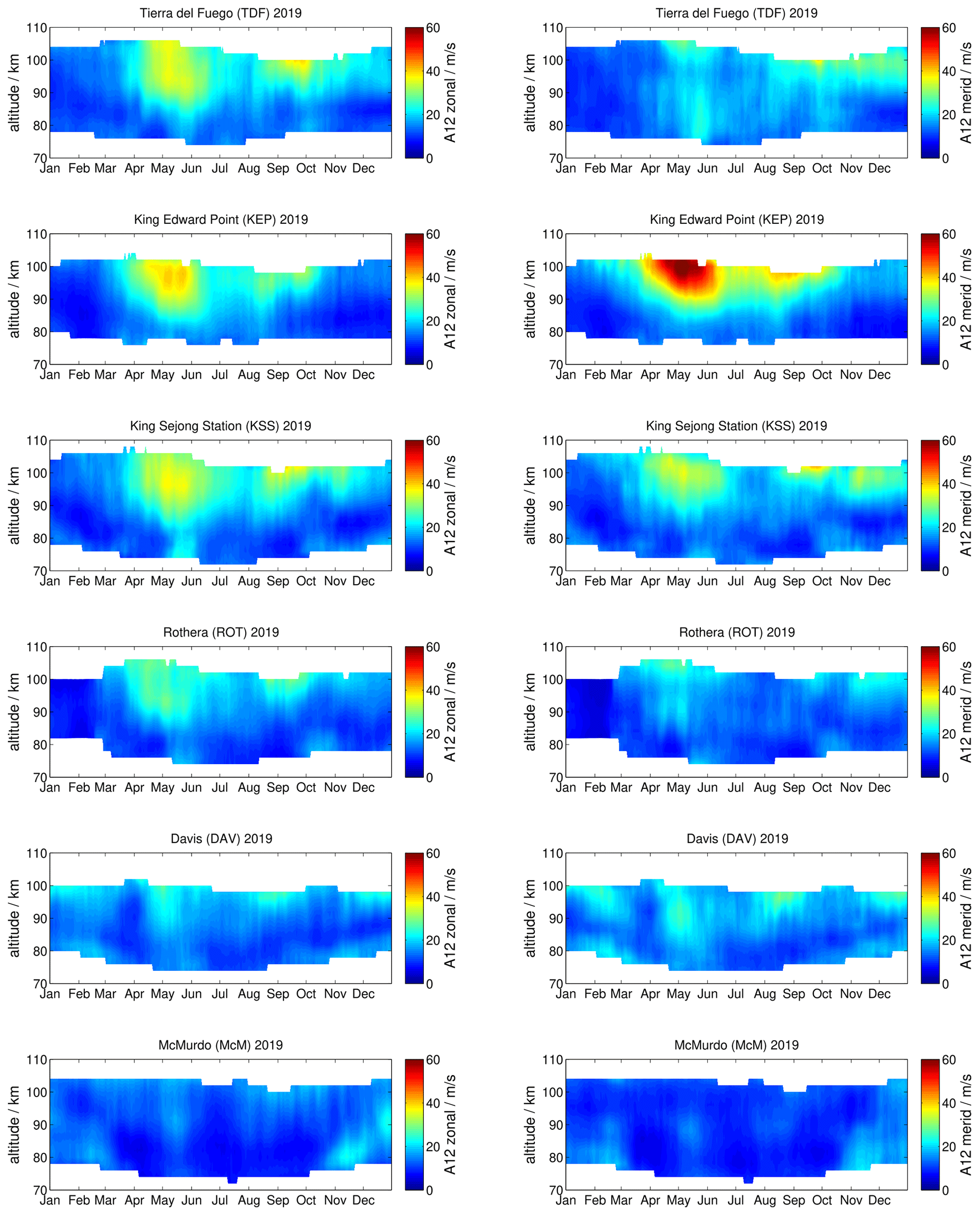
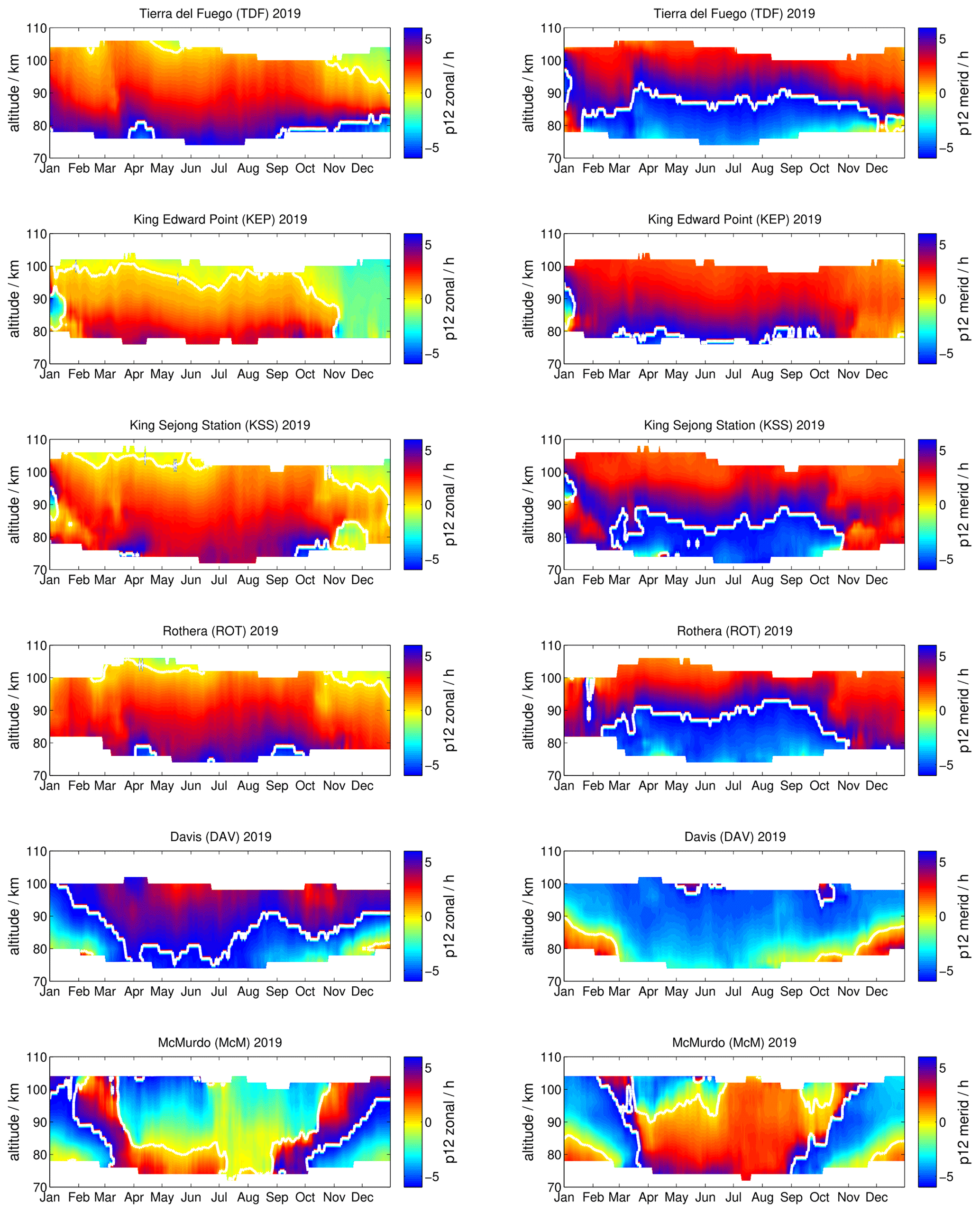
Figure 7 Comparison of semidiurnal tidal vertical wavelengths of (a) TDF, (b) KEP, (c) KSS, (d) ROT, (e) DAV, and (f) McM.

3.3 Semidiurnal tidal amplitudes and phases measured during 2019

At midlatitudes and high latitudes, semidiurnal tides are the dominating tidal wave during the course of the year (Hagan and Forbes, 2002, 2003). Figure 5 shows the vector-averaged semidiurnal tidal amplitudes measured by all six meteor radars using again a 30 d median shifted by 1 d in analogy to the mean winds and diurnal tides.

The seasonal structure of the semidiurnal tide reveals a rather interesting pattern for the SH. Semidiurnal tides measured at TDF, KEP, KSS, and ROT show some similarities for the zonal component, resulting in amplitudes with values below <10 m s⁻¹ during the summer months January to mid-March. From April to June, all four stations show a strong semidiurnal tidal activity, with amplitudes up to 40 m s⁻¹, another minimum of the tidal activity in July, and a secondary maximum from August to the end of the year. Furthermore, the tidal amplitudes show a decrease with increasing polar latitude, which is also observed at the Northern Hemisphere. However, the meridional semidiurnal tide shows a clear longitude dependence and asymmetry compared to the zonal tidal amplitudes, which was not reported previously (Conte et al., 2017). At the longitude of TDF and ROT the meridional tidal component is much weaker during April to June compared to the zonal. At KSS, which is further east, similar amplitudes for the zonal and meridional component are observed. This was also found at KSS in a previous study reporting the tidal amplitudes under solar maximum conditions, which resulted in larger amplitudes of the semidiurnal tide (Lee et al., 2013). KEP, which is 25^∘ eastward, shows the opposite behavior, and the meridional component of the semidiurnal tide reaches the highest amplitudes in April to June. Such differences with longitude might be related to the superposition of migrating and non-migrating tides (Murphy et al., 2006).

The semidiurnal tidal seasonal behavior observed at DAV looks quite different from the stations that are located further to the north. The amplitudes are much weaker and barely reach values of 25 m s⁻¹, and there are four periods during which an increased activity is observed, which are during January–February, May, August–September, and December. The largest tidal amplitudes are observed during May 2019.

Further to the south, at McM station, the semidiurnal tide exhibits only a very faint seasonal structure. Most of the time the amplitudes are below 10 m s⁻¹. Only during March, May, and November–December and below 90 km altitude are there periods where amplitudes exceed 10 m s⁻¹. This is surprising when we compare these values with measurements performed at geographically conjugate Northern Hemisphere latitude. For instance, at Svalbard (78.17^∘ N, 15.99^∘ E), the semidiurnal tide still reflects a similar seasonal activity to other polar and midlatitude locations (Wilhelm et al., 2019; Pancheva et al., 2020). This is obviously not the case in the SH and represents a remarkable interhemispheric difference.

Semidiurnal tidal phases are displayed in Fig. 6, where it can be seen that the semidiurnal tidal phases reflect similar features than those present in the amplitudes. TDF, KEP, KSS, and ROT show a very similar seasonal structure, indicating continuous changes of the tidal phases throughout 2019 at all altitudes. At DAV and McM, on the other hand, the observed phases indicate an even more pronounced seasonal structure and faster gradual phase drifts. In particular, at McM the phases appear to be more variable, which is likely due to the generally weaker amplitudes, pointing towards a much weaker and more intermittent excitation of the tides.

Comparing the seasonal phase behavior of the SH to that measured at conjugate latitudes in the Northern Hemisphere indicates that there are some differences. In the Northern Hemisphere, from midlatitudes to high latitudes, the semidiurnal tides show a seasonal asymmetry between the winter to summer transition and the fall transition (Portnyagin et al., 2004; Wilhelm et al., 2019; Stober et al., 2020). The fall transition is accompanied by a significant phase change from September to November, whereas in the SH this feature is very weak at TDF and ROT (March to May) and almost negligible for KEP and KSS.

Finally, we briefly discuss the presence of a potential lunar tide. Sandford et al. (2006, 2007) estimated the lunar tide amplitude from two northern hemispheric meteor radars and Davis MF radar in the SH and found values of 1–2 m s⁻¹, which is negligible compared to the typical GW amplitudes of about 20–30 m s⁻¹ for the resolved waves. However, Forbes and Zhang (2012) investigated a potential lunar tide amplification due to the Pekeris resonance. They found favorable conditions to shift the Pekeris peak towards the lunar tide periods M2 (12.42 h) and N2 (12.66 h), during the time of major sudden stratospheric warming in 2009 in the Northern Hemisphere, as only during the time of the wind reversal do the vertical temperature and wind structure satisfy the resonance conditions. Later, Zhang and Forbes (2014) argued that the Pekeris resonance peak is rather broad, and, thus, more or less each sudden stratospheric warming can cause a lunar tide amplification.

These reports triggered several studies investigating the lunar tide and its relevance for mesosphere dynamics. However, most of the observational diagnostics (wavelet or harmonic fitting) separating the lunar tide from the semidiurnal tide applied long windows of 21 d or even longer periods up to several months, assuming phase stability of the semidiurnal tide (Forbes and Zhang, 2012; Chau et al., 2015; Conte et al., 2017; He et al., 2018; Siddiqui et al., 2018). However, as shown in Fig. 6, the semidiurnal tidal phase shows considerable variability and seasonal changes, and, thus, the assumption of phase stability for the semidiurnal tide is not valid. Therefore, we performed a holographic analysis to test whether a temporally variable semidiurnal tidal phase could be misinterpreted as a lunar tide (see Appendix A1) (Stober et al., 2020) . In fact, the holograms often exhibit a shift towards the M2 frequency (12.42 h) uncorrelated with the lunar orbit. Given these results, and considering that there was only a minor stratospheric warming in September 2019 (Yamazaki et al., 2020), we consider the lunar tide to be a minor wave with a negligible amplitude compared to GWs, and we did not make an attempt to remove this tidal component in our Reynolds decomposition.

For the sake of completeness, we also estimated the vertical wavelengths of the semidiurnal tide, which is presented in Fig. 7. The vertical wavelength provides a good overview to identify potential changes in the Hough modes of the tide, which are solutions of the Laplace tidal differential equation (Lindzen and Chapman, 1969; Wang et al., 2016). The vertical wavelengths show a similar latitude and longitude dependence as already discussed for the semidiurnal tidal amplitudes and phases. The observations at TDF, KEP, KSS, and ROT indicate almost the same vertical wavelengths from March to October 2019 of about 70–100 km. This corresponds to the time with the largest semidiurnal tidal amplitudes. However, the seasonal summer months January–February and November–December show a longitudinal difference. KEP and KSS observe much longer vertical wavelengths of up to 1000 km during these months, compared to the stations located to the west. These very long vertical wavelengths are associated with times with a small semidiurnal tidal amplitude. The results obtained at DAV reflect a slightly different seasonal behavior. There, the longest vertical wavelengths are observed in March–April, followed by a stable hemispheric winter season until August, and a gradual decreasing of vertical wavelengths towards the end of the year. The results at McM show an even more complicated picture due to the almost vanishing semidiurnal tidal amplitudes. Only during the local summer months of January/February and November/December are meaningful vertical wavelengths derivable, with vertical wavelengths of about 70–100 km. It is also worth mentioning that the agreement between the zonal and meridional wavelengths is remarkable and provides further confidence in the applied ASF technique used for the Reynolds decomposition.

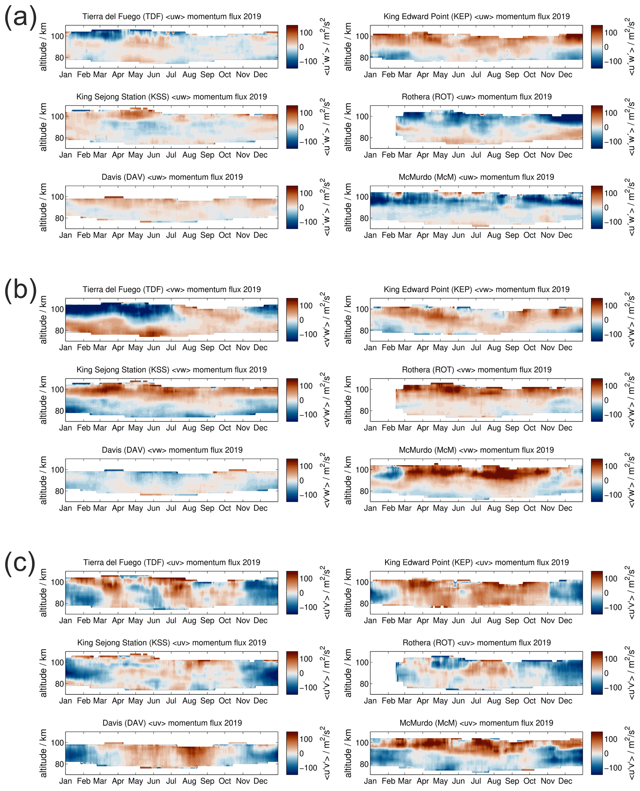
Figure 8 Comparison of vertical flux of zonal and meridional momentum and horizontal momentum flux for each station during the year 2019 for (a) the zonal momentum flux, (b) the meridional momentum flux, and (c) the horizontal momentum flux.

Figure 9 Same as Fig. 8 but for the (a) zonal, (b) meridional, and (c) vertical wind variances.

3.4 Reynolds stress components

Gravity waves are an essential driver of the MLT dynamics and variability, carrying energy and momentum from their source region to the altitude of their deposition. The breaking of GWs can trigger the generation of non-primary GWs, which again can propagate upwards (Becker and Vadas, 2018; Vadas and Becker, 2018), causing a complex interaction chain for the GW activity and the resulting forcing at the MLT. The acceleration and deceleration of the mean flow due to momentum and energy transfer by breaking GW can be estimated from the vertical gradient of the gravity wave momentum flux (Ern et al., 2011).

From our Reynolds decomposition and the retrieval, we determine three momentum fluxes, which are often referred to as the vertical flux of zonal momentum $<uw>$, the vertical flux of meridional momentum $<vw>$, and the horizontal momentum flux $<uv>$, where the $<>$ denotes temporal averaging.

Figure 8 shows all three momentum flux components as a 30 d median shifted by 1 d for the year 2019. There are three groups of panels presenting the vertical flux of zonal momentum (panel a), the vertical flux of meridional momentum (panel b), and the horizontal momentum flux (panel c). The stations are sorted according to their latitude within each panel to allow for an easier comparison between the sites. The results shown in this figure indicate that, for all six meteor radar observations, there is a characteristic seasonal pattern, with noticeable differences between the different locations.

The vertical flux of zonal momentum $<uw>$ is rather variable with longitude and latitude. Observations at TDF and ROT show some similarities regarding the seasonal structure. During the local summer, both indicate positive zonal momentum fluxes at the altitude of the zonal wind reversal. At higher altitudes, above 95–100 km, the zonal momentum flux reverses to negative values. The winter season appears to be more variable, which might be related to the minor warming in September 2019 and the wave activity before. To the east, at KEP and KSS, positive zonal momentum fluxes at the higher altitudes (95–105 km) are observed throughout the year but a rather different behavior during the local winter season at the altitudes below. In particular, at KSS a variable zonal momentum flux is measured that seems to be in better agreement with TDF and ROT results. Further to the south, at DAV and McM, the seasonal behavior of the zonal momentum flux seems to reflect the features that are already found at KEP but with different magnitudes.

The vertical flux of meridional momentum presented in Fig. 8 exhibits some longitudinal dependence. Observations at TDF and KEP show approximately the opposite vertical structure of the meridional momentum flux, pointing out that the meridional drag (acceleration and deceleration) reverses between their longitudes. Furthermore, results from KEP, KSS, and ROT show a good agreement of the vertical structure and seasonality of the meridional momentum flux throughout the year. Measurements at DAV still show some features of the seasonal meridional momentum flux behavior but with decreasing magnitude, while at McM, the results show once again a seasonal dependency comparable to that obtained at KEP.

Only the horizontal momentum flux $<uv>$ shows a similar seasonal behavior at TDF, KEP, KSS, ROT, and DAV, with negative values of −50 m² s⁻² during the seasonal summer and positive values in winter from April to October. The local winter shows more variability and a semiannual structure at some sites, similar to the mean zonal and meridional winds. At McM this seasonal variation is still visible but with a much weaker magnitude.

The seasonally dependent Reynolds stress components on the main diagonal of the tensor are also investigated. These terms are also often called zonal, meridional, and vertical wind variances. Figure 9 shows all three variances for each station. Note that the color scale for the vertical variances is 5 times smaller compared to the horizontal wind fluctuations. The zonal and meridional variances exhibit a seasonal structure and a rather obvious altitude dependence. The highest variances are observed at the highest altitudes, which is expected, considering that the Reynolds stresses are weighted by the atmospheric density, which decreases exponentially with altitude. It is also a common feature for all sites that the meridional velocity variances exceed the zonal fluctuations. The seasonal behavior of the zonal and meridional variances at all stations reflects a semi-annual variation, showing minimum variances during the equinoxes, when the mean winds are smallest at altitudes below 95–100 km. Above 100 km the seasonal characteristic appears to be less pronounced. The vertical wind variances are the most challenging values to retrieve. Their seasonal behavior is less obvious. However, the vertical wind variances also indicate increasing values with decreasing density. Results at McM are exceptional in this respect, and the vertical wind variances exceed the values that are derived at all other stations. At present we can only speculate on the source of these large values. A possibility is that McM lies underneath the auroral oval, and, thus, the altitudes above 90 km are strongly influenced by precipitating particles and associated effects like Joule heating that might trigger stronger vertical variations (Fong et al., 2014).

To gain confidence in our retrieved horizontal wind variances, we performed a test by estimating the GW wind variances of the resolved GWs directly. It is straightforward to derive a gravity wave residual from the hourly observed wind time series by subtracting mean winds and the diurnal and semidiurnal tide. Thus, we obtain a hourly time series of the GW residuals, which corresponds to the kinetic energy of the resolved GWs with periods longer than 2 h and horizontal wavelengths of more than 300 km, whereas the wind variances obtained using Hocking (2005) include the GW variances from all temporal and spatial scales. The GW variances from the residuals are shown in Fig. A2 in the Appendix.

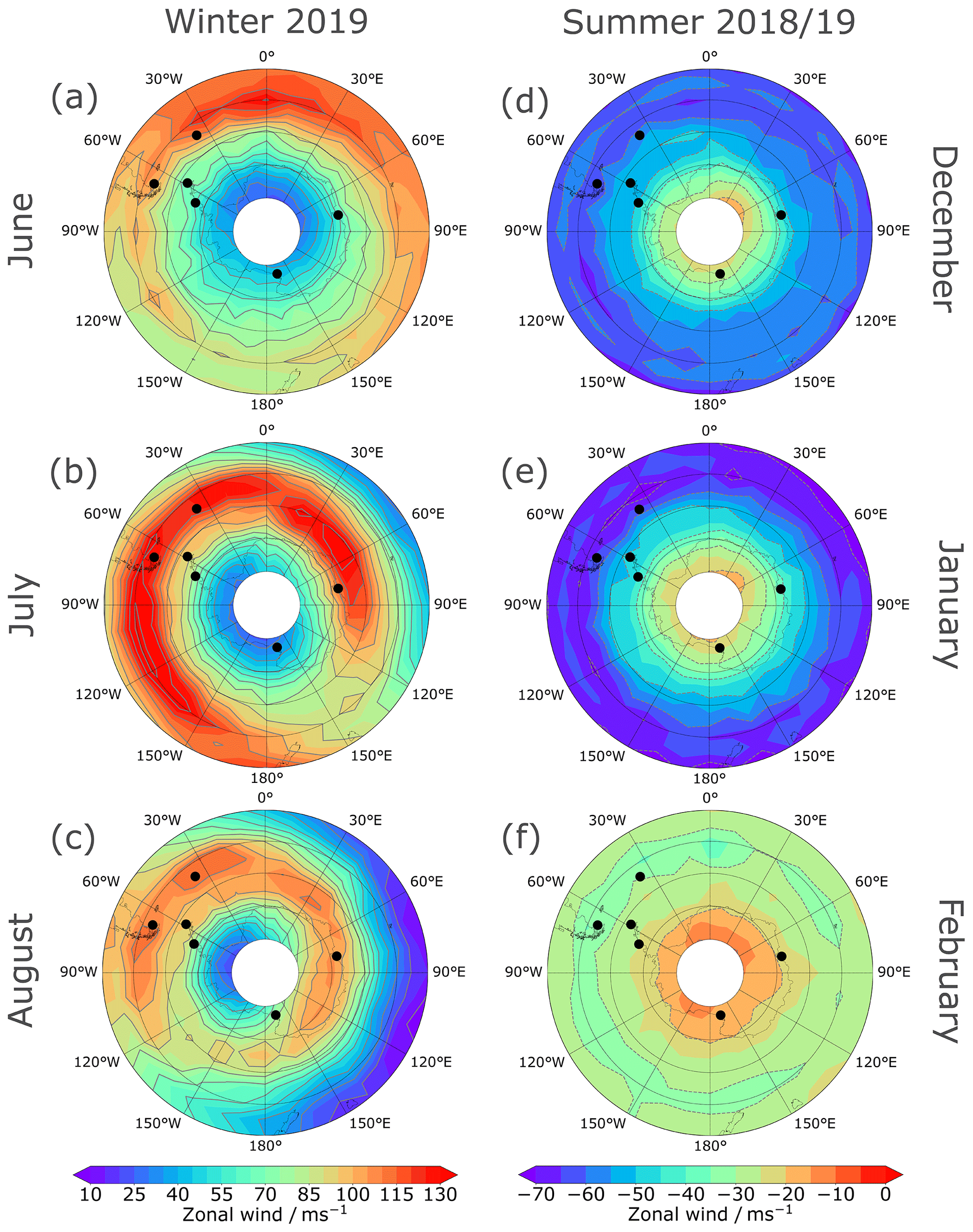
Figure 10 Monthly mean geostrophic zonal wind for the austral winter 2019 (a, b, c) and summer 2018/2019 (d, e, f), each averaged over the altitude range of its wind maximum (40–60 km for winter, 60–80 km for summer). Black dots mark the positions of the radar stations used here. Data are derived from MLS geopotential height data.

4 Discussion

Meteor radar observations of GW momentum fluxes have now been performed for more than a decade (Hocking, 2005; Fritts et al., 2010a; Placke et al., 2011b; Andrioli et al., 2013; de Wit et al., 2014, 2017). However, the results were not always conclusive and often difficult to interpret. Many of these former studies focus on understanding the method and how to optimize the analysis procedure (Fritts et al., 2010a, 2012b; Placke et al., 2011b; Andrioli et al., 2013; Placke et al., 2015a). Although the Reynolds decomposition appears to be straightforward, it can be challenging to do a proper and robust implementation and successfully separate the mean flow from the GW fluctuations. Fourier-based methods often require long averaging windows in order to get a proper resolution but do not capture the intermittency of the background sufficiently (see Fig. A3). For shorter windows the irregular sampling of meteors in time and altitude again causes deviations from a regular grid, and, additionally, data gaps have to be considered when applying wavelet or Fourier techniques. Another complication of the meteor radar momentum fluxes is that there are no “ground truth data” available to validate the measurements. Satellite observations provide only a total GW momentum flux without directional information obtained from temperature fluctuations after removing atmospheric tides up to wave number 4, assuming a stationary phase behavior over a couple of days (Ern et al., 2011; Trinh et al., 2018), and thus confidence in the methodology relies on tests with synthetic fields such as those presented in Fritts et al. (2010a, 2012a).

As we are mainly interested in the GW momentum flux and wind variances, we have to evaluate the presence of potential error sources in the Reynolds decomposition methodology carefully. In particular, atmospheric tides show a very intermittent behavior of the amplitude and phase, which causes some issues in the decomposition when long windows (several days/weeks or months) are used. Thus, we performed some tests to optimize the mean flow and tidal and GW decomposition, applying the ASF, a 1 d harmonic fit, and a 5 d harmonic fit (see Appendix A3). The comparison indicates that the Reynolds decomposition tends to be very sensitive to the applied technique, impacting the tidal mean flow and the gravity wave variances. Hence, the derived momentum fluxes and wind variances can be significantly different, even though the same or similar data sets are used. Previous studies used 4 d fits (de Wit et al., 2014) or S transforms (de Wit et al., 2017) to decompose the time series. In fact, the harmonic fits provide similar results compared to those obtained using Fourier-based techniques such as the S transform (Stockwell et al., 1996) or wavelets (Torrence and Compo, 1998) for the same averaging length.

Besides these technical aspects of the momentum flux and wind variance retrievals, the year 2019 was exceptional in the SH. The SH winter season was much more variable in August/September compared to previous years at TDF (climatology from 2008–2018) and was disturbed by a rare minor sudden stratospheric warming occurring in September (Yamazaki et al., 2020). This variability is reflected in the mean winds and the momentum fluxes, which show noticeable longitudinal and latitudinal differences, pointing towards an unstable and wobbling polar vortex. Figure 10 presents monthly mean geostrophic winds from the MLS (Matthias and Ern, 2018), averaged over the altitude range 40–60 km for winter months (a, b, c) and 60–80 km for summer months (d, e, f), the maximum wind region in each season (not shown). During winter the polar vortex is characterized by a strong longitudinal and latitudinal variation. This characteristic of the SH polar vortex is also found in the climatology of MLS for the SH. The strength of the polar vortex appears to be rather different, with longitude and month providing significant differences for the vertical propagation of GW and their encounters with critical levels, fostering wave breaking and the emission of non-primary waves due to localized body forces (Vadas and Fritts, 2001; Becker and Vadas, 2018; Vadas et al., 2018; Dong et al., 2020; Fritts et al., 2020).

Now we compare the observed momentum fluxes with a theoretical study at the SH in the context of non-primary waves (Becker and Vadas, 2018). The authors simulated GW drag (GWD) and momentum fluxes for the SH winter and show model outputs for a few days, which are qualitatively comparable to our observations. One major effect of the non-primary waves was a significant increase of the zonal and meridional GWD at 60^∘ W and latitudes between 50–70^∘ S. Our meteor radar observations reflect this increased zonal wave drag for all stations falling into this geographic region (TDF, KSS, ROT) by a considerably different meridional mean wind pattern during June–August compared to the other stations (KEP, DAV). Further, the model simulations resulted in a weaker effect for the meridional GWD, and, thus, the zonal winds are not as different between the stations. Comparing the observed momentum fluxes between these simulations and our observations, we found a reasonable agreement for KEP and DAV. Most of the time, the model predicts an eastward zonal momentum flux and a northward meridional momentum flux for the winter months for all longitudes, except for the mountain wave gravity hotspots around 60^∘ W. At this longitude, the model suggests more variable conditions due to the temporal variable mountain wave excitation, which triggers the body forces at the stratosphere and, thus, the secondary or non-primary wave generation (Vadas and Becker, 2018). As a result, stations in Argentina (TDF) and on the Antarctic Peninsula (KSS, ROT)sometimes show southward meridional momentum fluxes as westward zonal momentum fluxes for the winter months.

We also computed the zonal and meridional GWD from the vertical structure of the retrieved momentum fluxes. The KMCM (Kühlungsborn Mechanistic Circulation Model) sometimes reached values of almost 600 m s⁻¹ d⁻¹ for the zonal GWD and about 1000 m s⁻¹ d⁻¹ for the meridional GWD (Becker and Vadas, 2018). Our observations resulted in similar values on average, which supports the finding that the model and observations are sensitive to a rather similar part of the relevant gravity wave scales with respect to the periods and horizontal wavelengths.

Recent studies on momentum flux spectra using general circulation models suggest that most of the energy of the GW at the MLT is found at periods between 4–12 h and at horizontal wavelengths of λ_h≈1000 km (Shibuya and Sato, 2019). These scales are covered by our variance and momentum flux retrievals due to the Reynolds decomposition performed, and, thus, our results should be representative as integral over the most relevant gravity wave periods and horizontal scales. However, WACCM (Whole Atmosphere Community Climate Model) simulations suggested a leading order contribution of gravity waves between 20–200 km, which are also present in the obtained momentum fluxes. Considering the modeling results from Vadas and Becker (2018), Becker and Vadas (2018), and Shibuya and Sato (2019), as well as our observations of the SH momentum fluxes for all stations, the leading order effect for the momentum budget is given by larger horizontal scale waves and inertia GW periods, which are characteristic properties of non-primary waves.

This polar vortex wobbling in 2019 is essentially modifying the mesospheric gravity wave activity and the resulting momentum flux at the altitude of the wave breaking in the mesosphere and above. Characteristics of GWs in the MLT strongly depend on their vertical propagation path and the background wind field along this path, which efficiently alters the amplitude growth of the gravity waves depending on their phase velocity relative to the mean flow. On the other hand, breaking gravity waves deposit momentum on the mean flow and, thus, enhance, weaken, or shift the polar vortex, contributing further to the wobbling, especially in the mesosphere. For example, the wind maximum in the meteor radar zonal winds (see Fig. 2) was at lower altitudes in June but at upper altitudes in July and August for most of the stations. One explanation of this phenomenon could be that the polar vortex in the upper stratosphere–lower mesosphere (see Fig. 10) was relatively weak in June for most of the stations, while it was considerably stronger in July and August in particular. This hypothesis is confirmed by the observations obtained at KEP, where stronger winds are already observed in the upper stratosphere and lower mesosphere in June, resulting in a higher wind maximum compared to the other stations. Furthermore, there are considerable longitudinal differences of orographic gravity wave sources in the SH, already resulting in some asymmetry at stratospheric altitudes.

During the summer months the differences in the zonal wind between the different stations in the mesosphere are much smaller than in winter (see Fig. 10), resulting in smaller differences between the stations in the meteor radar observation window (see Fig. 2).

In particular, the SH winter season shows remarkable longitudinal and latitudinal changes in the strength of the zonal wind velocities (see Fig. 10). Observations with TDF and the KEP radar, although at the same latitude, show that the polar vortex is rather different at each longitude, significantly modifying the conditions for vertical GW propagation, and, thus triggering differences in the altitude of the momentum flux deposition. Furthermore, it is likely that both stations experience the effect of different GW sources. ROT and KSS are also reflecting significant differences in the momentum fluxes, which are partly explainable by the mesospheric zonal wind field, which shows a strong gradient above the Antarctic Peninsula, leading to differences of the polar vortex above KSS and ROT.

The most consistent results among the various locations investigated in this study are obtained in the horizontal momentum fluxes $<uv>$ and the wind variances. TDF, KEP, KSS, ROT, and DAV observe a very similar seasonal behavior, and only the strength of the flux differs between the sites. This is also the case for the wind variances, which are very consistent between the meteor radars, providing confidence in the retrievals.

The orography around the meteor radars only plays an indirect role in the observed mesospheric momentum fluxes and wind variances. The observed total flux above the station is the result of all gravity waves that propagate into the mesosphere, independent of their origin (e.g., jet instabilities, convection, orography or non-primary waves). Satellite observations of the total momentum flux showed a significant GW hotspot around the Andes and Antarctic Peninsula at the stratosphere (Ern et al., 2011). However, with increasing altitude, this momentum flux forms a plume stretching downwind of the Andes and Antarctic Peninsula, and, at the mesosphere–lower thermosphere, one finds more or less a longitudinal band of the momentum flux confined to the latitudinal band between 40–65^∘ S (Trinh et al., 2018). GW-resolving GCMs indicate that the zonal and meridional momentum flux shows a latitudinal and longitudinal structure (Becker and Vadas, 2018), with multiple sign reversals of the momentum flux within this latitude band. In particular, the signs of the resulting momentum flux are opposite between the Antarctic Peninsula and the Andes around TDF. Furthermore, the momentum fluxes exhibit a reversal of the GW drag between TDF and KEP at the mesosphere, although both locations are at the same latitude.

5 Conclusions

This study presents an overview of gravity wave momentum fluxes and wind variances at the MLT in the SH from the midlatitudes at TDF, Argentina, and KEP to the polar latitudes of DAV and McM Antarctic stations as well as King Sejong Station and ROT on the Antarctic Peninsula for the year 2019. The year 2019 was exceptional, and, in particular, the hemispheric winter season appears to be more disturbed than previous years, resulting in a rare minor stratospheric warming in September.

We performed a detailed analysis of the mean zonal and meridional wind for the year 2019 to explore the longitudinal and latitudinal differences. We noticed significant differences on relatively small regional scales, for instance between KSS and ROT. In addition, we found a strong dependence of the zonal and meridional wind pattern during the SH winter season, indicating an asymmetric structure of the polar vortex at the MLT. This asymmetry was verified by MLS geostrophic zonal wind observations at the stratosphere and mesosphere, which revealed longitudinal differences of the intensity as well as an altitude dependence of the polar vortex, leading to temporal and spatially variable filter conditions for the vertical propagation of gravity waves. These results are consistent with the predictions made from model simulations about the secondary or non-primary wave generation due to breaking mountain waves above the gravity hotspots in Argentina and the Antarctic Peninsula.

The derived mean daily wind climatologies for the year 2019 provide convincing evidence that the meridional wind and to a weaker extend the zonal winds are disturbed during the winter season due to orographically generated mountain waves, causing non-primary wave emissions at the stratosphere. This asymmetry in the zonal and meridional winds sustains a polar vortex wobbling in the SH that can be found consistently in the climatologies from MLS and at TDF and DAV.

Furthermore, we investigated the diurnal and semidiurnal tidal seasonal variation of the amplitudes and phases for all six stations to assess longitudinal and latitude differences similar to the mean winds. The diurnal tide showed a consistent behavior of the amplitude and phases measured at TDF, KEP, KSS, ROT, and DAV and entirely different seasonal response over McM. Diurnal tidal phases appeared to be most variable during the local winter season, where the smallest amplitudes are observed. Semidiurnal tides indicated a more complex seasonal structure, exhibiting a strong difference in amplitude between the zonal and meridional component for TDF, KEP, and ROT, which was not reflected by the semidiurnal tidal phases. In addition, with increasing southern latitudes, the amplitude of the semidiurnal tide decreases and shows a different seasonal structure at DAV and basically vanishes over McM. The seasonal characteristic of vertical wavelengths observed by the meteor radars between 80–100 km for the hemispheric winter season from mid-February to October 2019 at TDF, KEP, KSS, and RO is very consistent and takes values of 80–100 km. Moreover, there was a tendency of increased vertical wavelengths during times with very small semidiurnal tidal amplitudes.

Finally, we retrieved the wind variances at all stations. These wind variances exhibit a seasonal behavior with minimum variances during the equinoxes. In general, the meridional wind variances exceed the zonal components. Besides some differences in the absolute values of the wind variances, all observations feature remarkable similarities throughout the year 2019.

Appendix A

A1 Holographic analysis

The holograms shown in Fig. A1 are computed from the semidiurnal tidal phases in the complex domain to account for phase wrapping. As a time-dependent phase corresponds to a frequency shift, it is straightforward to estimate the potential Doppler shift of the tidal frequency. Colors towards red indicate a shift towards lower frequencies, whereas a shift towards blue indicates higher frequencies in analogy to optical Doppler measurements. The method is presented in more detail in Stober et al. (2020). It is evident from this figure that the natural variability of the semidiurnal tide already covers the frequency of the predicted lunar tide during a Pekeris resonance (12.42 h) (Forbes and Zhang, 2012; Zhang and Forbes, 2014). However, these frequent phase shifts appear to be uncorrelated with the lunar orbit and can occur throughout the year at all meteor radar locations without satisfying the vertical conditions of the winds and temperature fields required for the Pekeris resonance.

A2 Gravity wave residual kinetic energies

The Reynolds decomposition with the ASF can also be used to separate the resolved gravity waves from tides and the daily mean winds. Figure A2 shows the gravity wave residuals after subtracting the daily mean zonal and meridional wind, as well as the diurnal and semidiurnal tides. This gravity wave residual essentially contains the inertia gravity waves with periods up to 16 h that are not tides. The separation between tide and gravity wave is done by the vertical wavelength.

A3 Reynolds decomposition comparison of ASF and harmonic fitting

The Reynolds decomposition is a very important element in the momentum flux and wind variance measurements. Therefore, we tested different methods to perform the Reynolds decomposition. Figure A3 shows a comparison of the ASF (upper two panels), a harmonic fit with a 24 h window (central panels), and the harmonic fit with a 5 d window (lower two panels). The left column always shows the reconstructed time series using a daily mean winds and the diurnal, semidiurnal, and terdiurnal tide. The right column shows the resulting gravity wave residuals. The 2D ASF performs well in recovering a very smooth tidal field and even changes in the tidal phases with altitude. The main difference compared to the 24 h fit is given in a cleaner removal of a potential inertia gravity wave contamination of the fitted tidal fields due to gravity waves with rather short vertical wavelengths. A 5 d harmonic fit increases the gravity wave residuals significantly, as phase variations of the tide within the long window are no longer sufficiently captured.

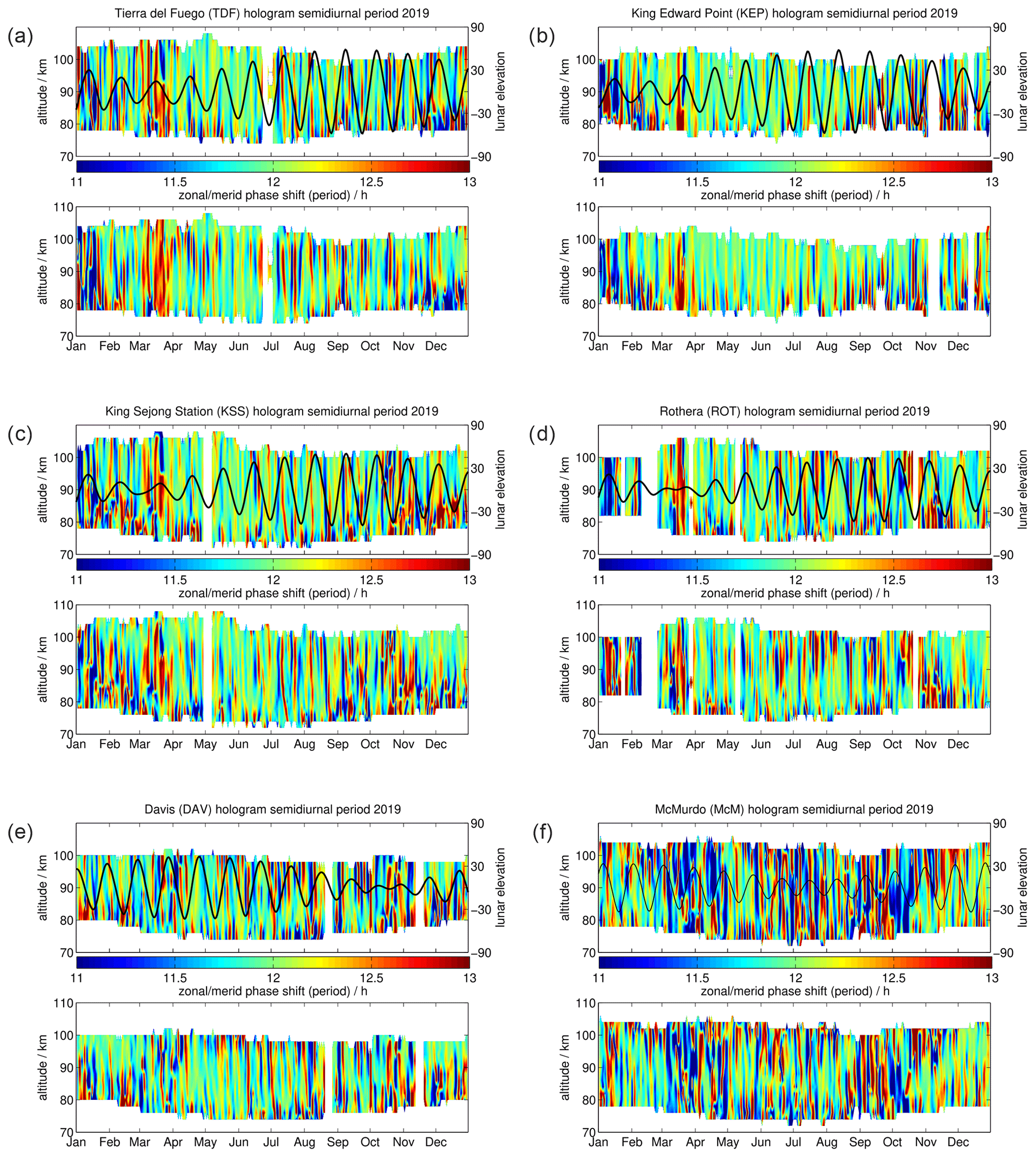
Figure A1 Holographic analysis of the semidiurnal tidal variability and lunar elevation angle (thin black line) for each station during the year 2019 for (a) TDF, (b) KEP, (c) KSS, (d) ROT, (e) DAV, and (f) McM.

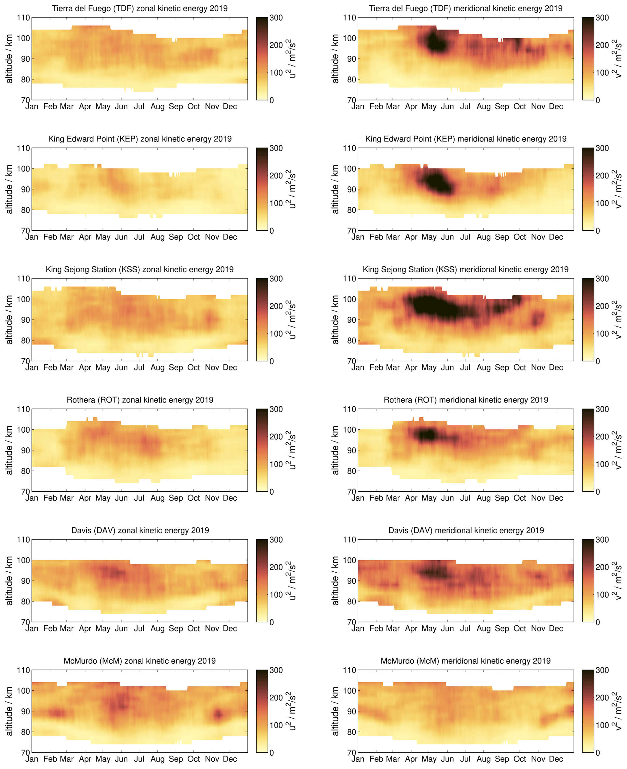
Figure A2 Kinetic gravity wave energy as determined for the resolved waves from the ASF for each station during the year 2019. Same as Fig. 2.

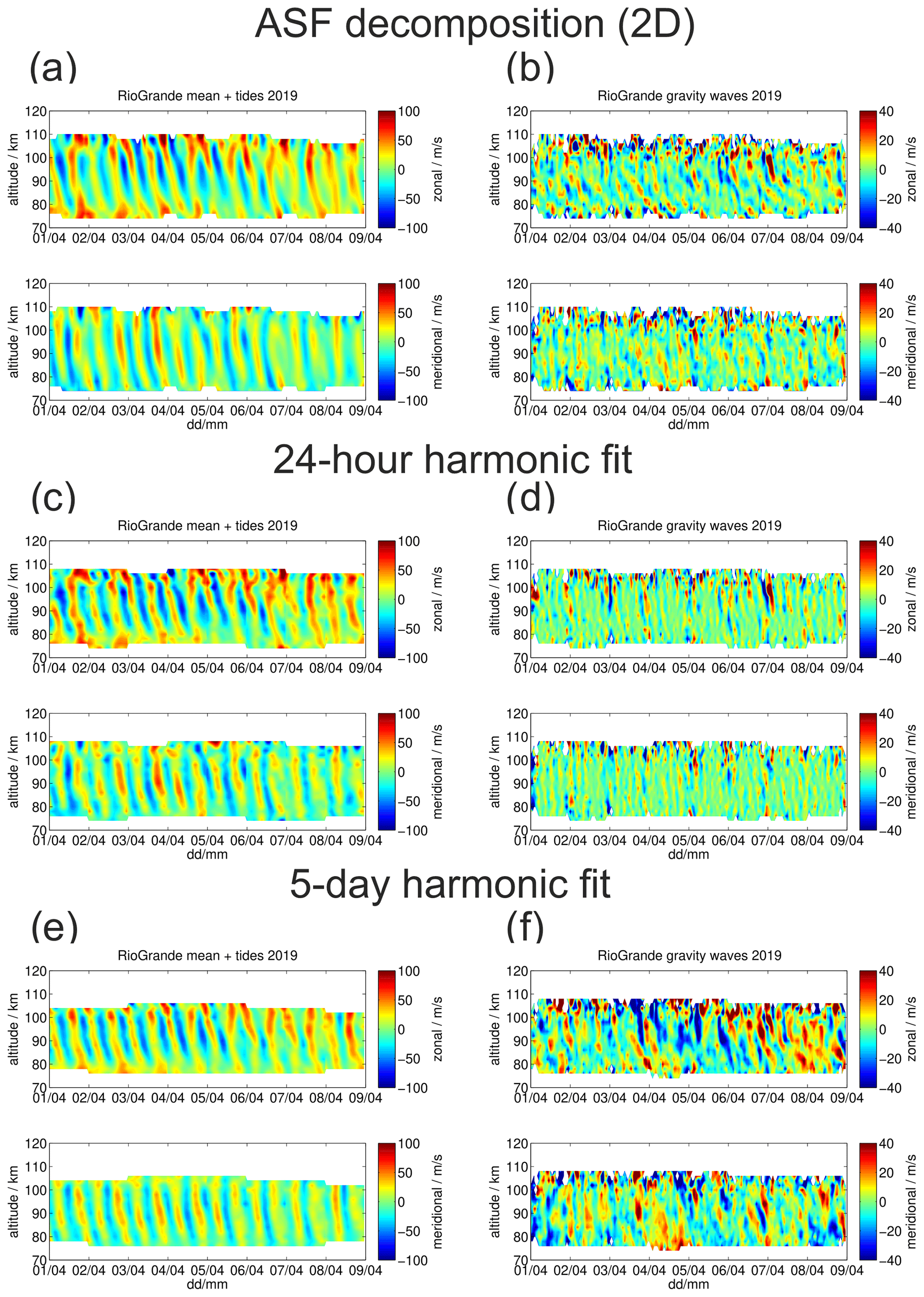
Figure A3 Comparison of different Reynolds decomposition for 8 d at TDF (Rio Grande) to underline the sensitivity of the applied method in deriving gravity wave fluctuations. Panel (a) shows the ASF reconstructed daily mean plus diurnal, semidiurnal and terdiurnal tide time series. Panel (b) presents the gravity wave residuals. Panels (c) and (d) show the same but for a 24 h harmonic fit and panels (e) and (f) for a 5 d harmonic fit.