Semiannual variation of Pc5 ultra-low frequency (ULF) waves and relativistic electrons over two solar cycles of observations: comparison with predictions of the classical hypotheses

Pc5 ULF (ultra-low frequency) waves can energize electrons to relativistic energies of >2 MeV in geostationary orbits. Enhanced fluxes of such electrons can induce operational anomalies in geostationary satellites. The variations of the two quantities in timescales ranging from days to solar cycles are thus of interest in gauging their space weather effects over different time frames. In this study, we present a statistical analysis of two 11-year solar cycles (cycles 22 and 23) of data comprising the daily relativistic electron fluence observed by Geostationary Environment Satellites (GOESs) and daily Pc5 ULF wave power derived from auroral zone magnetic observatories in Canada. First, an autocorrelation analysis is carried out, which indicates a 27 d periodicity in both parameters for all solar phases, and such a periodicity is most pronounced in the declining and late declining phase. Also, a 9 and 13 d periodicity are seen in some years. Then, a superposed epoch analysis is performed to scrutinize semiannual variation (SAV), which shows that fluence near the equinoxes is 1 order of magnitude higher than near solstices, and Pc5 ULF wave power is 0.5 orders of magnitude higher near the equinoxes than near the solstices. We then evaluate three possible SAV mechanisms (which are based on the axial, equinoctial, and Russell and McPherron effect) to determine which one can best explain the observations. Correlation of the profiles of the observational curves with those of the angles that control each of the SAV mechanisms suggests that the equinoctial mechanism may be responsible for the SAV of electron fluence, while both the equinoctial and the Russell and McPherron mechanisms are important for the SAV of Pc5 ULF wave power. Comparable results are obtained when using functional dependencies of the main angles instead of the angles mentioned above. Lastly, superposed curves of fluence and Pc5 ULF wave power were used to calculate least-square fits with a fixed semiannual period. Comparison of the maxima and minima of the fits with those predicted by the three mechanisms shows that the equinoctial effect better estimates the maxima and minima of the SAV in fluence while for the SAV in Pc5 ULF wave power the equinoctial and Russell and McPherron mechanisms predict one maximum and one minimum each.

1 Introduction

Relativistic electrons with energies >2 MeV can penetrate the surface of a satellite and cause internal charging that can induce satellite operational anomalies, as conclusively demonstrated by Wrenn (1995). Internal charging by relativistic electrons not only causes satellite operational anomalies that are a nuisance to satellite operators but can also render the complete failure of a satellite, as exemplified by the consecutive outages of Telesat Canada's Anik-E1 and E2 geostationary satellites on 20 January 1994 that wreaked havoc in communication across Canada for hours (Baker et al., 1994a, b; Lam et al., 2012). There are other serious satellite incidents due to internal charging by relativistic electrons, such as the Anik-E1 failure on 26 March 1996 (Baker et al., 1996). The intensification of relativistic electrons that can cause satellite problems has been shown to be associated with Pc5 ultra-low frequency (ULF) waves (Rostoker et al., 1998; Mathie and Mann, 2001; Mann et al., 2004; Simms et al., 2014; Lam, 2017). The acceleration mechanisms of relativistic electrons attributable to Pc5 ULF waves can be due to magnetic pumping (Borovsky, 1986; Liu et al., 1999), drift-resonant acceleration (Elkington et al., 1999), transit-time acceleration (Summers and Ma, 2000) and the popular radial diffusion (e.g., Falthammar, 1968; Schulz and Lanzerotti, 1974; Perry, 2005; Ozeke et al., 2014). No matter what the actual acceleration mechanism or process is, Lam (2017) has shown that Pc5 ULF wave power has the potential to predict relativistic electrons that can harm satellites. It is, therefore, pertinent to peruse the time variations of Pc5 ULF waves and relativistic electrons together in detail in order to appraise their space weather effects over different time assemblies.

In this work we analyze ground-based Pc5 ULF wave powers, which are a manifestation of Pc5 ULF waves and relativistic electrons at geostationary orbit, focusing on their time variations from a few days to a solar cycle (SC). An extended analysis is carried out for a particular kind of variation known as the semiannual variation (SAV). SAV is an annual phenomenon, characterized by maximum levels of activity near equinoxes and minima near solstices, and it can be detected in a diverse set of solar–terrestrial measurements (Azpilicueta and Brunini, 2011, 2012; Vichare et al., 2017; Bai et al., 2018), including relativistic electrons of the outer Van Allen belt (Baker et al., 1999; Li et al., 2001; Kanekal et al., 2001) and ULF waves (Sanny et al., 2007; Rao and Gupta, 1978). In the first case, Baker et al. (1999) used measurements of both the low-altitude Solar Anomalous and Magnetospheric Particle Explorer (SAMPEX) and high-altitude POLAR spacecraft to calculate quarterly averages centered at the equinoxes and solstices. They found that the fluxes were nearly 3 times higher at the equinoxes than at solstices, which means a semiannual modulation in these measurements (McPherron et al., 2009). Moreover, SAMPEX observations were also used by Kanekal et al. (2010) to study the dependence of the SAV in relativistic electrons, with a wide range of L shells covering the descending and ascending parts of a SC. Their results showed that the flux peaks were delayed about 30 d from the times of the nominal equinoxes during the descending phase. But, in the ascending phase, the lag times were asymmetrical for both equinoxes.

In the case of ULF waves, Sanny et al. (2007) examined the seasonal and diurnal pattern of ULF wave powers, using magnetic measurements from Geostationary Environment Satellites (GOESs) sensors. They studied Pc3, Pc4 and Pc5 pulsations, which all clearly exhibit the June and/or July minimum. They also identified a strong local minimum in Pc4 band power around noon, whereas the minima of the Pc5 and Pc3 bands appeared to be distributed on the dayside. All the frequency bands had elevated power levels around local midnight. An older work in which a SAV is reported in Pc5 pulsations was published by Rao and Gupta (1978). They found the SAV to be particularly evident in the morning hours, close to 08:00 ± 1 h local time (LT).

There are three mechanisms that are commonly referred to in the literature to explain the SAV, and each one seems to be controlled by an angle. The first mechanism is known as the axial hypothesis, and the angle is the Earth's heliographic latitude. This angle reaches maximum absolute values about 14 d before the equinoxes (see Table 5) when the Earth approaches the high-speed solar wind regime such as the sunspot regions (Cortie, 1912) or coronal holes. The high solar wind speed originating from these regions might be the driver of the enhancements in the activity. On the contrary, the Earth crosses regions of slow-speed solar wind approaching the solstices, at the proximity of the Sun's equator, and then there is minimum activity (Phillips et al., 1995).

The second mechanism is known as the Russell and McPherron (RM) hypothesis (Russell and McPherron, 1973), which establishes that there is a varying probability of a southward-directed component of the interplanetary magnetic field throughout the year. This leads to a different probability of magnetic reconnection between the interplanetary magnetic field and the terrestrial magnetic field lines at the nose of the magnetopause. Near the equinoxes (solstices), the probability is maximum (minimum). The relevant angle is the angle between z^GSM and z^GSEq (GSM – geocentric solar magnetospheric; GSEq – geocentric solar equatorial coordinate system).

The last mechanism is known as the equinoctial hypothesis (Bartels, 1932). Boller and Stolov (1970) showed that, in theory, the Kelvin–Helmholtz instability originated by the viscous-like interactions between the solar wind and the magnetosphere along the flanks of the magnetosphere predicts a semiannual pattern with instability maxima (minima) near the equinoxes (solstices). This is thought to be the physical process behind the equinoctial theory. The controller angle is the one delimited by the solar wind (SW) direction and the Earth's dipole.

A main objective of this work is to test which one of these mechanisms better predicts the SAV that we find in Pc5 ULF wave powers and in relativistic electrons. The procedure involves the comparison between observational curves and the shape of the relevant angles of each mechanism. This method has been applied before to look for the dominant mechanism in the geomagnetic activity (Roosen, 1966; Cliver et al., 2002), finding that the equinoctial and RM effects are the dominant ones and the axial effect is the least important. This paper not only extends their work in magnetic activity in terms of Pc5 magnetic wave powers but also includes relativistic electrons in geostationary orbits. The consolidation of the two quantities in a single study on their SAVs and other periodicities over two solar cycles elucidates their space weather effects under different temporal contexts.

2 Data

2.1 GOES relativistic electrons

As internal charging by relativistic electrons on satellites located at geosynchronous orbit is a function of integrated flux over a time period, we use daily fluence values, which are an accumulation of fluxes over 24 h, to represent the electron variations in this work. Specifically, we analyzed fluences of relativistic electrons with energies >2 MeV derived from flux measurements on board the National Oceanic and Atmospheric Administration's (NOAA) GOES. GOESs are in geostationary orbit about 35 790 km above Earth's surface in the equatorial plane at 6.6 R_E.

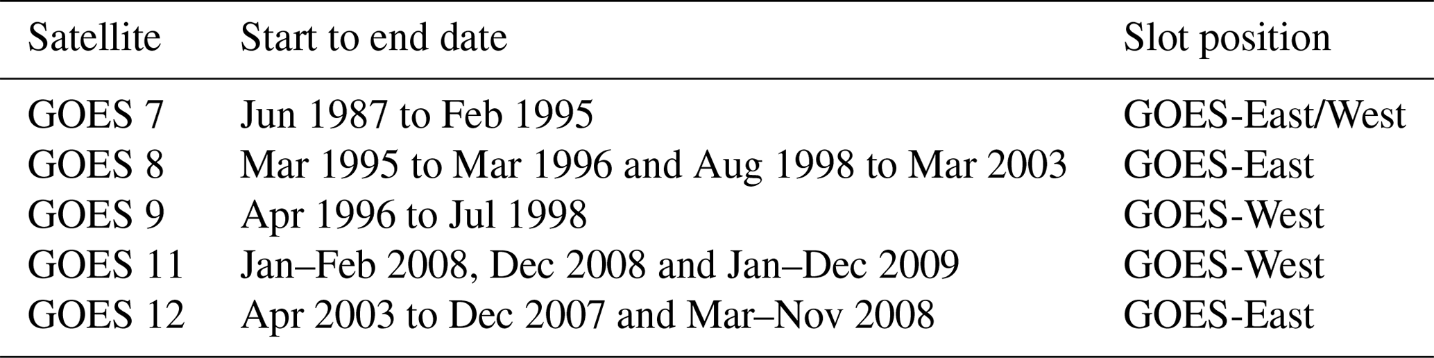
The data span SCs 22 and 23 from June 1987 to December 2009. The same data suite has been used previously to study Pc5 ULF wave powers and relativistic electrons by Lam (2017), who provided details on GOES and GOES data. Briefly, GOES is referred to as GOES-East when located at 75^∘ W and GOES-West when located at 135^∘ W, and the directional integral flux of >2 MeV electrons with a cadence of 5 min measured by GOES's electron sensor is the source of the fluence data.

Table 1 spells out the specific GOESs used in this work, with their time coverage and East or West allocation. The rationale behind the choice of these satellites is given in Lam (2017). Briefly, only satellites designated as GOES primary were used in this study (GOES can be a primary or secondary satellite). The specific GOESs were chosen for their time coverage to ensure that the 23 years of data fully cover different solar phases of the two solar cycles.

Table 1 Satellite data used in this study.

2.2 Pc5 ULF wave powers

To study ULF waves in the Pc5 frequency band, we generate a time series of daily Pc5 ULF wave powers referred to as Pc5 powers, using Canadian geomagnetic data collected by the Canadian Magnetic Observatory System (CANMOS; Lam, 2011). The geomagnetic data cover the same period as the electron data described in Sect. 2.1. The hourly values of Pc5 power derived using the X component (northward component) of the Earth's geomagnetic field recorded at 1 min intervals were used in this study. The 24 hourly powers of a universal time (UT) day were added to obtain the daily power. In Lam (2017), daily power was the mean of the hourly powers in a UT day after the hourly powers in the midnight sector were excluded to avoid the contamination of substorms to “pure” Pc5 ULF waves. However, in order to investigate the semiannual variations fully in this study, the daily power includes contributions from the midnight sector so that all magnetic fluctuations in the Pc5 spectrum (Jacobs et al., 1964) in a UT day are considered. We refer the reader to Lam (2017) for more detail on the methodology used to obtain Pc5 power from the raw geomagnetic data. Briefly, the minute data were first band-pass filtered, and then a fast Fourier transform was computed using a Hanning window to obtain the Pc5 power spectral estimates.

The CANMOS observatories selected to calculate Pc5 power (see Table 2) are located in the Canadian auroral zone, close to the footprints of the magnetic field lines threading GOES, in order to relate ground magnetic variations with relativistic electrons near the geostationary orbit. As can be seen from the last column of Table 2, the data come primarily from the Fort Churchill station (FCC) that is located at a geographic longitude of 94.1^∘ W, which is approximately midway between GOES-East and GOES-West. Where there were gaps or spikes in FCC data, Yellowknife (YKC) data were used. When both FCC and YKC data were absent or not usable, Poste-de-la-Baleine (PBQ) data were used. When data from FCC, YKC and PBQ were not available, data from Baker Lake (BLC) and Cambridge Bay (CBB) at the fringe of the auroral zone near the cusp were used to fill in the data gap. It can be seen from Table 2 that FCC and YKC together cover ∼94 % of the total days processed, with FCC contributing most of the data.

Many studies have been carried out using Pc5 power derived from a single magnetic station in the auroral oval, as in this study (Glaßmeier, 1988; Trivedi et al., 1997; Mathie and Mann, 2001; Mann et al., 2004). As pointed out by Lam (2017), Kozyreva et al. (2007) noted that improvements made by the global ULF wave index did not change the basic features of its temporal variations and that the results of the works of Mathie and Mann (2001) and Mann et al. (2004) obtained from nonglobal ULF wave power remain valid. It is therefore justifiable to use the Pc5 power from a single auroral zone station to generate a large dataset for the statistical study in this work.

Table 2 Coordinates of CANMOS observatories used in this work.

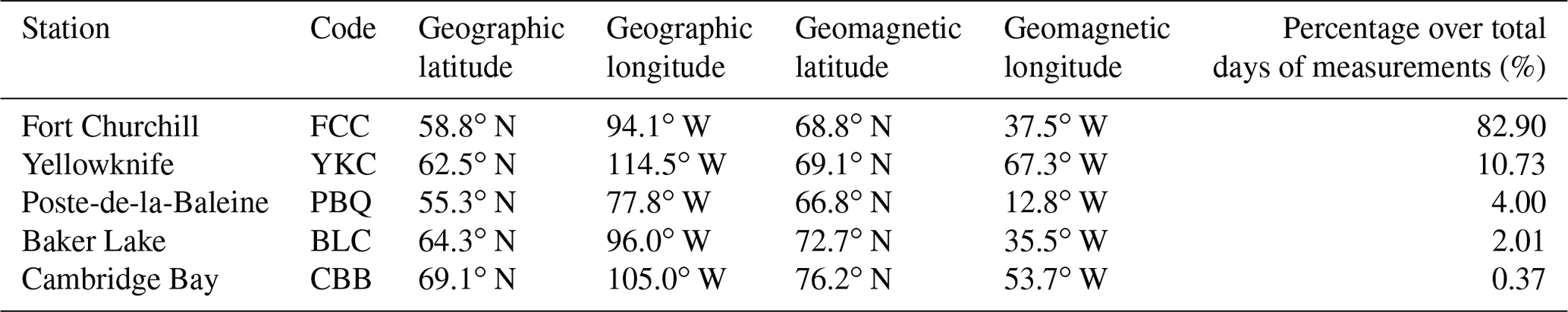
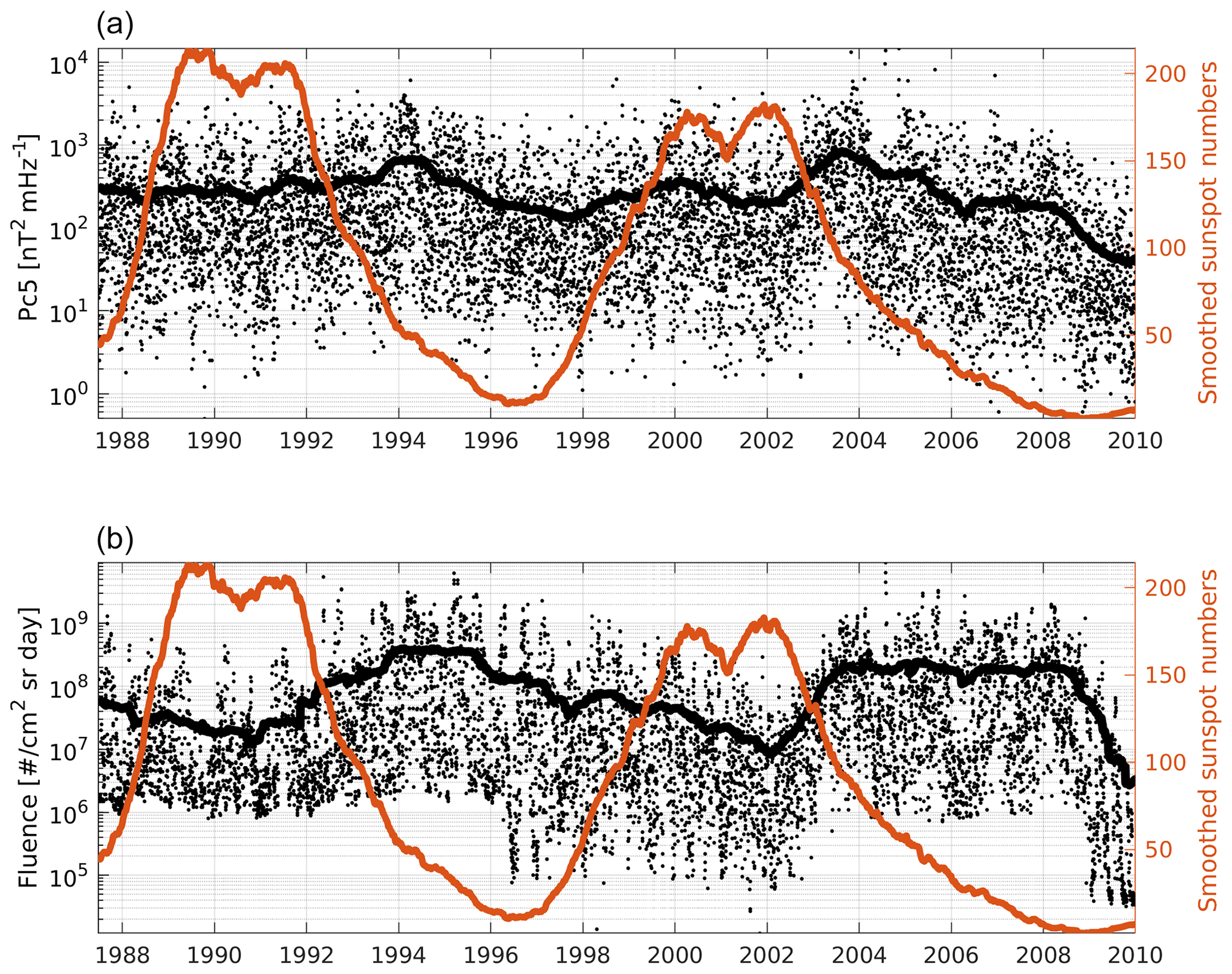
Figure 1 (a) Pc5 power daily values represented as black dots. The thick black curve is the Pc5 power smoothed with a 365 d moving average. (b) Fluence daily values represented as black dots. The thick black curve is the fluence smoothed with a 365 d moving average. The orange curve corresponds to the yearly smoothed sunspot numbers sequence.

3 General characteristics of Pc5 power and fluence in SCs 22 and 23

Figure 1 presents an overview of the complete Pc5 power and fluence daily values plotted as black dots. This figure echoes the trends delineated in Fig. 1 of Lam (2017), in which the daily values exclude midnight sector contributions, as mentioned earlier.

The thick black lines are the 365 d moving average of the Pc5 power and fluence. The smoothed sequence of daily sunspot numbers has also been added (orange curve) to represent the SC, which is useful when referencing the variations of the parameters to a specific SC phase.

The smoothed curves of Pc5 power and fluence can be used to highlight the underlying trends. For example, they indicate high levels during the descending phases of both cycles. Differences in trends at different phases of an SC can also be seen. Although there appear to be minor variations in the trends between Pc5 power and fluence (e.g., Pc5 increasing while fluence is decreasing in the early portion of SC 23 and Pc5 leveling while fluence is depressing around the SC 22 maximum), the gross features of their evolution, in both SCs, appear to be similar.

To see the relationship between Pc5 power and electron fluence, Fig. 2 shows their variations in logarithmic scale (log) for 1996 and 2007 during the lower portion of the descending phase of SC 22 and 23, respectively. The x axis corresponds to the day of year (DOY). The peaks and valleys in Pc5 power and fluence seem to follow each other, with a lag of about a couple of days in fluence peaks with respect to Pc5 power peaks. This time shift is clearer for 2007 than for 1996 and was studied in detail by Lam (2017), who concluded that Pc5 power can potentially be used to predict electron fluence 2 to 3 d in advance, before the enhancements in electron fluence at geostationary orbit, and also that the lag is smaller for extremely high fluence values.

Besides showing the relationship between Pc5 power and electron fluence, Fig. 2 also indicates that, in 1996, fluence values clearly demonstrate a SAV pattern, which is not readily discernible at first glance when looking at other years. Furthermore, both years show regular variations in the two parameters. The SAV and the regular variations, as exemplified here, will be further investigated statistically in the sections below.

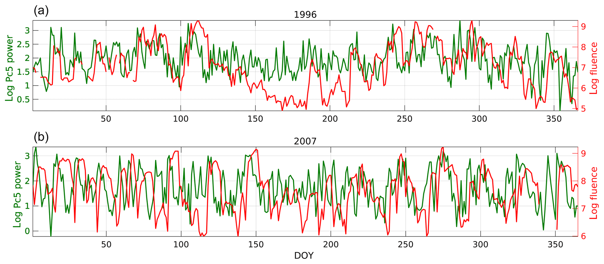
Figure 2 Fluence (red curve) and Pc5 power (green curve) values in 1996 (a) and 2007 (b). The peaks and valleys of Pc5 power and fluence seem to follow each other closely, especially in 2007.

3.1 Dominant periodicities

3.1.1 Autocorrelation functions

In order to investigate the dominant periodicities in Pc5 power and electron fluence, we calculated the autocorrelation function (ACF) of the logarithm of both parameters for specific years corresponding to different phases of a solar cycle. To establish whether a value of correlation at a certain lag was significant or not, a criterion based on a Student's test (or “t test”) on the correlation coefficient r was adopted. Following Rodgers and Nicewander (1988), the hypothesis of null correlation (r=0) is rejected when r satisfies the following:

$$\begin{array}{}\text{(1)}& \left|r\right|>{\displaystyle \frac{t}{\sqrt{N-\mathrm{2}+t^{\mathrm{2}}}}},\end{array}$$

where N is the length of sequence in days, and t is the quantile of a Student's distribution (t distribution), with N−2 degrees of freedom and a significance level of 1 %. If the hypothesis cannot be rejected, r is statistically equivalent to zero and considered not significant.

Figures 3 and 4 present the ACFs of the logarithmic Pc5 power and fluence, respectively, for different phases of both SCs (22 and 23) as a function of lag in days. In addition, 1 representative year of the ascending, maximum, descending, late descending and minimum phases was selected based on the shape of the sunspot numbers in Fig. 1. The years corresponding to each phase are explicitly shown in the figures.

Since N remains constant for every lag value, there is a region in the plots inside which r should be considered statistically null, as delimited by two critical values of correlation (CVCs). This region is bounded by two horizontal black lines located at ±CVCs. The obvious maximum value at lag 0 was excluded from the figures in order to accommodate an appropriate scale.

Figure 3 Autocorrelation functions (ACFs) of Pc5 power for different phases of the SC 22 (a) and 23 (b) as a function of lag in days. The horizontal black lines are the critical values of correlation (CVCs).

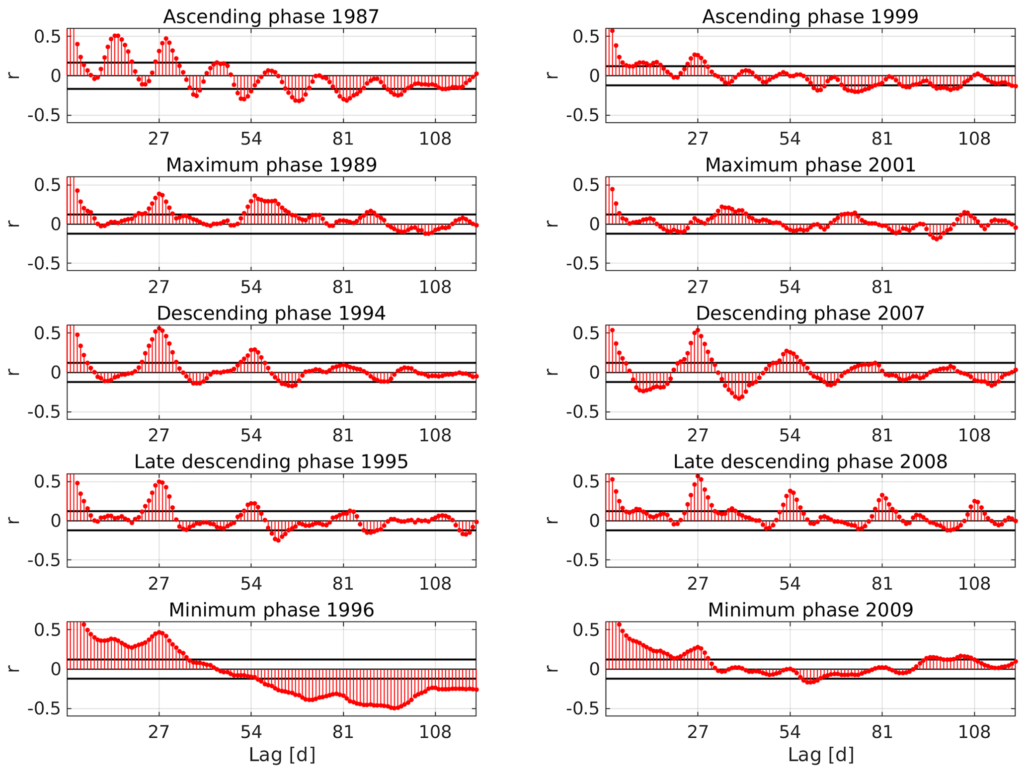
Figure 4 ACFs of electron fluence for different phases of the SC 22 (a) and 23 (b) as a function of lag in days. The horizontal black lines are the CVCs.

In the ascending phase, Pc5 power shows two clear peaks that exceed the CVCs around the 13 and 29 d lag in 1987. The r values reach 0.3 in 1987. Similar peaks are discernible in 1999, though at a slightly different lag (e.g., peaking at 27 d lag instead of at 29 d lag in 1987). These peaks are also present in fluence. The peak around the 29 d lag in SC 22 or the peak around the 27 d lag in SC 23 approximates the solar synodic period (T_syn≃27.27 d), which is due to the solar rotation, and impinges a quasi-periodic 27 d variation upon many solar–terrestrial parameters (Poblet and Azpilicueta, 2018). The values over the CVCs at ∼13 d lag could be related to the 13 d periodicity that previous authors have found (e.g., Mursula and Zieger, 1996; Lam, 2004).

During the maximum phase, the peaks present in the ascending phase cannot be seen in Pc5 power as all the variations in 1989 and 2001 (Fig. 3) are bounded by CVCs, while in fluence the 27 d peak is still quite prominent in 1989 but less obvious in 2001 (Fig. 4).

During the descending and late descending phases, the ACFs show not only the strongest values of correlation at the 27 d lag but also high values at ∼54, ∼81 and ∼108, which are all multiples of 27. The value at day 27 reaches a maximum of 0.57 in 2008 for both Pc5 power and fluence. A peculiar characteristic that can be seen in Fig. 3 in 2008 is that the correlation values exceeding CVCs have a 9 d recurrence.

Although the peaks at multiples of 27 are quite sharp in the descending phase, the ACFs have smooth transitions between positive and negative values over the course of 27 d, suggesting that the solar rotation generates a 27 d variation with a sinusoidal-like pattern in these years, as seen in the smooth progression of the anticorrelation values near the ∼13 d lag. On the contrary, in the late descending phase the transitions between the peaks at multiples of 27 differ in both parameters. In fluence, we can deduce that the 27 d variation acts more like a spike, owing to the flat correlation values in between solar rotations, whereas in Pc5 power the lower harmonic, with a period of ∼9 d in 2008, is evident.

In the minimum phase, ACFs in fluence exhibit continuously moderate correlation values above CVCs between lags 0 and ∼30 and a negative trend thereafter, with a reversal at large lag days between 1996 and 2009. For Pc5 power during the minimum phase, 1996 shows the persistent 27 d peak, which is present during other phases, as mentioned above, and that peak is also present in 2009, though at a lower r.

3.1.2 A synopsis of the periodicities of Pc5 power and electron fluence over two solar cycles

The analysis developed in Sect. 3.1.1 provides a partial view of the periodicities as it only relates to specific years in different SC phases. In this section, we present the ACFs of each year of SC 22 and 23 together to trace the evolution of the periodicities throughout the two SCs. They are illustrated in 2D plots shown in Fig. 5, which displays a synopsis of the periodicities of Pc5 power and electron fluence for the entire two solar cycles. The horizontal axis corresponds to the years and the vertical axis to the lags (between 0 and 120 d). Figure 5a–b show the Pc5 power and fluence ACFs, respectively, where the neighboring values have been interpolated to visualize the trends better. In Fig. 5c–d, the plots are repeated for clarity, with values of $\left|r\right|$ not exceeding $\left|\mathrm{CVC}\right|$, shown as white bins.

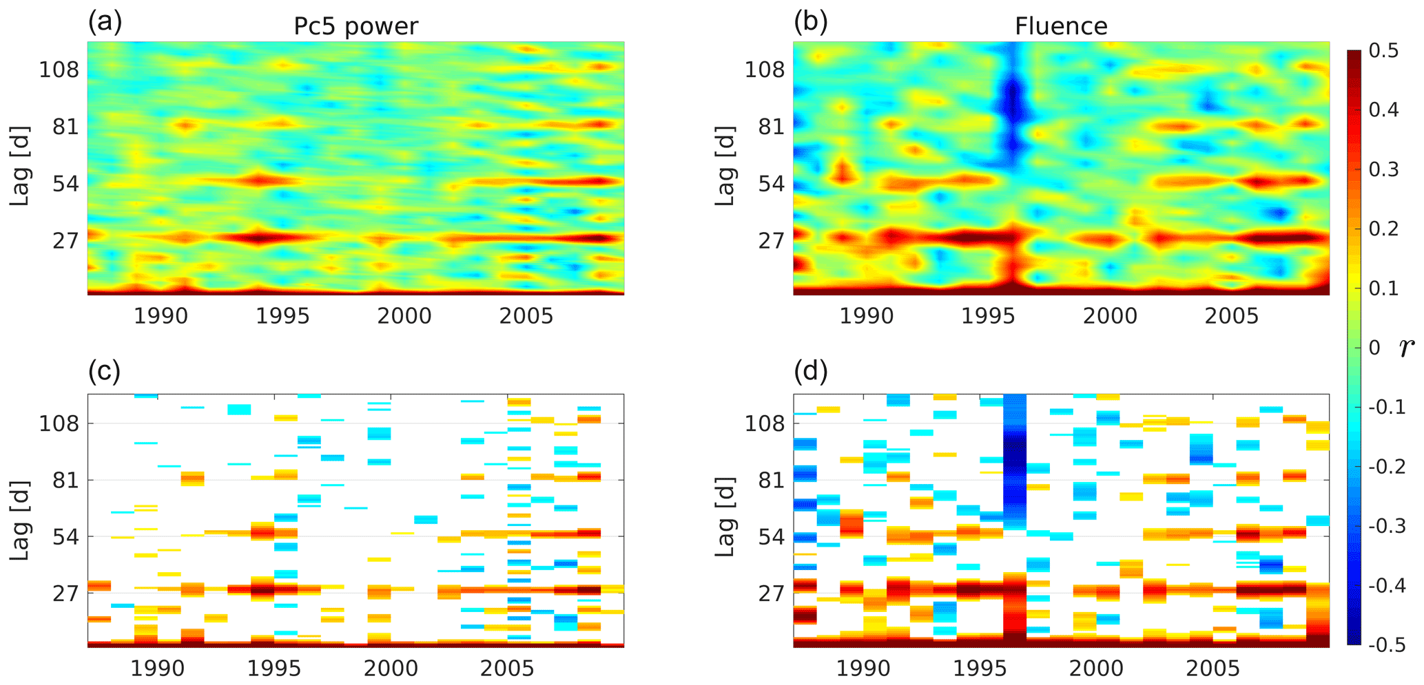
Figure 5 The 2D plots of ACFs of every year. In the horizontal axis is the year and in the vertical axis is the lag (between 0 and 120 d). Panels (a) and (b) show the Pc5 power and fluence ACFs, respectively, with the neighboring values interpolated. White bins in panels (c) and (d) belong to $\left|r\right|$ values that do not exceed $\left|\mathrm{CVC}\right|$.

From the almost continuous horizontal line of high correlation values centered at 27 d lag in all the panels, we can infer that the 27 d periodicity is the most prominent regular periodicity detected in Pc5 daily power as well as in fluence. In fact, all years, except 1988 (ascending phase), 1998 (ascending phase) and 2001 (maximum phase), have values above CVCs around the 27 d lag. The years of 1994, 1995, 2006, 2007 and 2008 exhibit the strongest 27 d recurrence pattern with the highest correlation values. All these years belong to the descending or late descending phase. The enhancements at multiples of 27 are also very clear. As Fig. 5c–d show, they are dominant in the descending phase and absent in the ascending and maximum phase for both parameters.

The present understanding of the effects of the 27 d variation that the solar rotation generates in the geospace environment can be used in the interpretation of our results. The regions known as corotating interaction regions (CIRs; Tsurutani et al., 2006) are particularly important since they produce recurrent disturbances in geomagnetic activity and in other geospace phenomena. CIRs are formed when solar wind high-speed streams emanating from coronal holes into the interplanetary space catch the slow-speed streams, creating regions of enhanced density and magnetic fields.

During the declining phase of the SC, CIRs are particularly prominent as a result of the expansion of coronal holes (CHs) to lower latitudes, generating a well-developed sector structure in the heliospheric magnetic field. In this SC phase, the ACFs of Pc5 power and fluence show the strongest values of correlation at a 27 d lag and the clearest 27 d periodicity that repeats for several solar rotations. However, the fact that the ACF peaks above CVCs occur not only during the descending phase but also during other phases suggests that the 27 d variation in Pc5 power and fluence could also be due to smaller irregularities, other than CHs, capable of persisting for more than a solar rotation in the corona.

The peaks with a 9 d period seen in 2008 for Pc5 power (shown clearly in Fig. 3) can also be seen in 2004 and 2005, as observed in Fig. 5d. All of these years belong to the declining and late declining phases of SC 23. On the contrary, only 2005 shows this periodicity clearly in fluence.

There are some previous reports of the 9 d recurrence in solar variables. For example, Ram et al. (2010) developed a comprehensive analysis of the solar rotation period and its subharmonics in the fractional area that CHs occupy at a fixed region of the Sun and also in the solar wind velocity. They found that both parameters exhibit subharmonics with a period of 9 d during the declining and minimum phase of SC 23. Also, Temmer et al. (2007) and Lei et al. (2008) studied the prominent 9 d periodicity in the solar wind velocity in 2005, probing that it was caused by a triad of CHs separated by $\sim \mathrm{120}{}^{\circ }$ in heliographic longitude that were active for several rotations. So the 9 d periodicity that we find in Pc5 power and fluence seems to be supported by prior investigations.

Finally, note that 1996 in fluence shows a different behavior to all the other years. This is evident when looking at this particular year in Figs. 2 and 4. The different behavior of the fluence values in 1996 is related to the distinct semiannual pattern of that year, as alluded to earlier in Fig. 2.

4 Semiannual variation (SAV)

In order to investigate the SAV in Pc5 power and electron fluence, we performed a superposed epoch analysis of the logarithmic daily values of both parameters using the entire suite of two solar cycles of data. The zero epoch was simply the first DOY, and we calculated the median for each DOY from DOY 1 to DOY 365 (the extra day corresponding to leap years was not used due to its negligible effect on the results). Owing to the length of the observations, there are ∼23 values (corresponding to about 23 years) for each DOY to use in the calculation of the median. The results can be seen in Fig. 6a–b, which show the superposed curve as black lines corresponding to Pc5 power and electron fluence, respectively. We chose the median over the mean for the superposition, since it is not skewed so much by extremely large or small values, and it may give a better approximation of the “typical” value for each DOY. The upper and lower limits of the gray band mark the quartiles.

The 30 d running average of the curves with the median is also added in Fig. 6a–b (green line for Pc5 power and red line for electron fluence, respectively) and will be referred to as Pc5_SAV and Fl_SAV, respectively. The 30 d moving average serves to diminish the strong 27 d variation since this is the most prevalent periodicity in both Pc5 power and fluence values, as shown in Sect. 3.1.

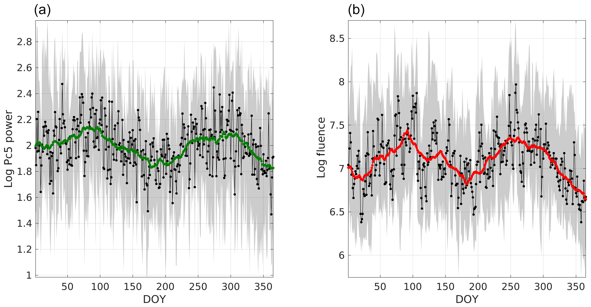
Figure 6 Superposed epoch analysis of the logarithmic values of Pc5 power (a) and fluence (b). The median and quartiles are illustrated as a black curve, lower limit and upper limit of the gray band, respectively. The zero epoch is the first day of year (DOY), and the green and red curve are the 30 d running average of the median curve (Pc5_SAV and Fl_SAV).

Pc5_SAV and Fl_SAV demonstrate a clear SAV, with maxima around the equinoxes and minima near the solstices. Although not as clear, the SAV pattern can also be seen in the curves associated with the median and quartiles. The peak-to-peak variation of Fl_SAV is of 1 order of magnitude, approximately, and of ∼0.5 orders of magnitude for Pc5_SAV. There are differences and similarities in the SAV of Pc5 power and fluence, and they will be discussed in Sect. 4.1 and 4.3 below. Those sections will explore, in more detail, the phases and profiles of the SAV in both parameters, but more importantly, they will be compared with the phases and profiles predicted by the three classical hypotheses (introduced in Sect. 1) so that the dominant mechanism can be ascertained.

4.1 Annual profiles

In this section we compared the profiles of the angles that govern each SAV mechanism (introduced in Sect. 1) with the profiles of Pc5_SAV and Fl_SAV. For the axial hypothesis, we considered the daily values of the Earth's heliographic latitude (ψ). For the equinoctial hypothesis, we used the daily mean values of the angle delimited by z^GSM and the Earth's dipolar axis denoted by ϕ that is equivalent to the magnetic solar declination (with the same annual variation). Finally, for the RM effect we took the daily mean values of the angle between the z^GSM and z^GSEq axes that is measured in the y–z plane of both coordinate systems (GSM and GSEq), referred to as θ. Figure 7 schematically shows these three angles in the Sun–Earth environment, where the gray plane is the solar equatorial plane.

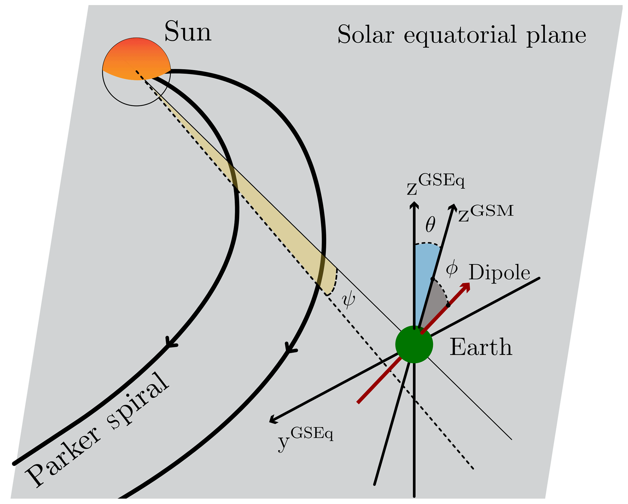
Figure 7 ϕ, θ and ψ in the Sun–Earth environment (see text for details). Parker spirals lie approximately in the solar equatorial plane that is shown in gray. GSEq and GSM are the geocentric solar equatorial and geocentric solar magnetospheric coordinate systems, respectively.

Figure 8 presents the annual profiles of $\left|\mathit{\theta }\right|$, $\left|\mathit{\psi }\right|$ and $\left|\mathit{\varphi }\right|$. The $\left|\mathit{\varphi }\right|$ scale is inverted in the figure in order to adequately identify the semiannual pattern in the three angles. As we are using daily mean values, the high-frequency oscillations due to diurnal variations of ϕ and θ vanish. The three curves present a different overall shape for the seasonal modulation. For example, the equinoctial mechanism anticipates sharper maxima and broader minima than the axial and RM hypotheses. The maxima and minima of the three angles fall on different dates and have different variation ranges, namely $\sim \mathrm{23}{}^{\circ }$ for $\left|\mathit{\varphi }\right|$, $\sim \mathrm{26}{}^{\circ }$ for $\left|\mathit{\theta }\right|$ and $\sim \mathrm{8}{}^{\circ }$ for $\left|\mathit{\psi }\right|$. Note that $\left|\mathit{\theta }\right|$ is defined considering the geocentric solar equatorial (GSEq) coordinate system and not the geocentric solar ecliptic (GSE) as in some works (Lockwood et al., 2016). This causes $\left|\mathit{\theta }\right|$ to reach slightly different values at the maxima. Considering GSEq over GSE also delays the location of the maxima for several days and is more consistent with the original definition of the RM effect reported in Russell and McPherron (1973, see, for example, Fig. 4 in that paper).

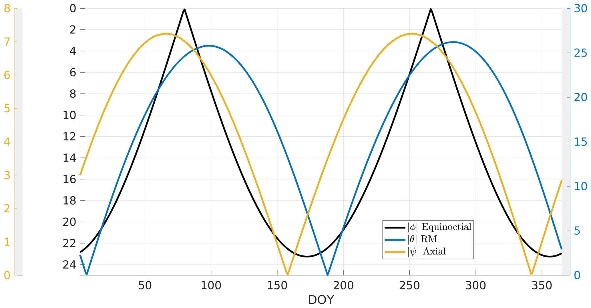
Figure 8 Absolute value of the angles that might control the SAV. ϕ, θ and ψ are associated to the equinoctial, RM and axial hypotheses, respectively.

To compare the shape of the angles with FL_SAV and Pc5_SAV, we applied a 30 d running average to the curves in Fig. 8. The results can be seen in Fig. 9, where FL_SAV and Pc5_SAV are also illustrated at 3 d intervals. Since five time series are plotted together in this figure, the 3 d interval helps to improve the visualization of all of them. It can be seen that FL_SAV and Pc5_SAV follow the semiannual pattern better between DOYs 180 and 365, approximately. In fact, between DOYs 200 and 250, Pc5_SAV almost overlaps the smoothed inverted $\left|\mathit{\varphi }\right|$ curve. On the contrary, between DOYs 1 and 179 the agreement between observed and predicted semiannual patterns diminishes. This is clearly seen between DOYs 1 and ∼60 where FL_SAV and Pc5_SAV reach higher values than the curves of the angles. There is, however, a good agreement between $\left|\mathit{\theta }\right|$ and the observed curves in the interval of DOYs given by ∼150–179. Also, on DOY 147, FL_SAV shows a peak that is lower than the maximum falling near the first equinox DOY. Note that, as can also be seen in Fig. 6, near this equinox FL_SAV shows a sharper maximum than Pc5_SAV.

Some authors have used these three angles (or similar ones) in the past to test SAVs detected on magnetic indices. For example, Roosen (1966) used the ap index from 1932 to 1966 and determined that the annual pattern of the smoothed index presents greater similarity with the smoothed equinoctial angle than with the smoothed axial angle. Cliver et al. (2002) extended that comparison utilizing the 30 d smoothed patterns of the three angles and the aa magnetic index from 1868 to 1998 to obtain high values of correlation with the smoothed $\left|\mathit{\theta }\right|$ – but especially with the smoothed inverted $\left|\mathit{\varphi }\right|$.

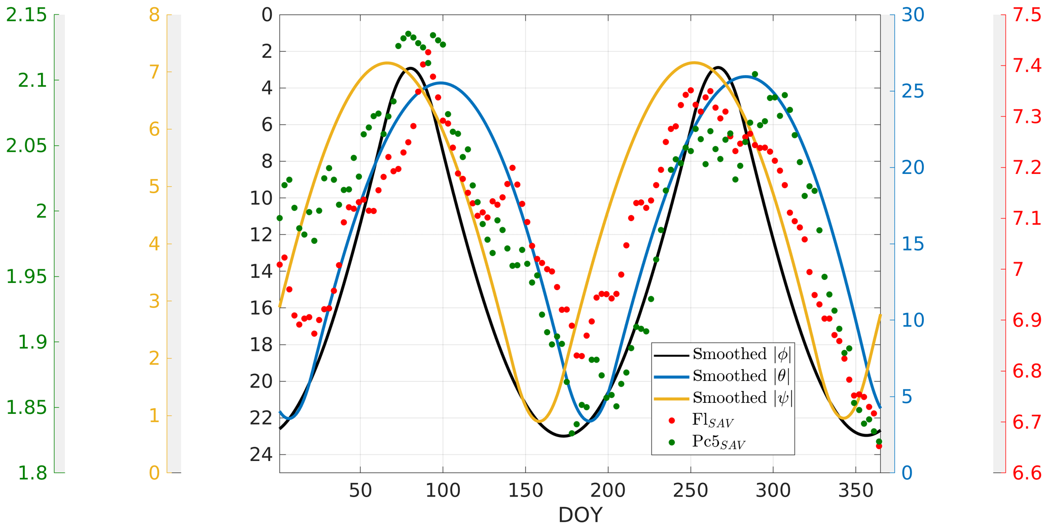
Figure 9 Smoothed absolute value of the angles that control the SAV. ϕ, θ and ψ are associated to the equinoctial, RM and axial hypotheses, respectively. FL_SAV and Pc5_SAV have also been added and plotted at 3 d intervals. The 3 d interval helps to improve the visualization of the five time series.

We calculated the correlation values between our observational curves (FL_SAV and Pc5_SAV) and the smoothed angles, and the results are summarized in Table 3. The equinoctial hypothesis seems to dominate the SAV in fluence since the correlation value between the smoothed $\left|\mathit{\varphi }\right|$ and FL_SAV profiles reaches the minimum value of −0.87, meaning that they anticorrelate very well. There is a lower fidelity of FL_SAV with the RM profile (r=0.82). As regards Pc5_SAV, the profiles of both hypotheses (equinoctial and RM) show comparable correlation (anticorrelation) values, suggesting that the two mechanisms could play equally important roles in the generation of the SAV in Pc5 power. The profile of the axial hypothesis presents the lowest agreement with both parameters (0.69 for FL_SAV and 0.64 for Pc5_SAV).

4.2 Functional dependencies of the angles

In principle, it should be possible to use the profiles of the three angles to determine which is the dominant mechanism, but a better approximation may be achieved by considering the functional dependencies of each angle. In this section, we evaluate the functions of ϕ or θ proposed by different authors (Svalgaard, 1977; Perreault and Akasofu, 1978) in the past for studying the SAV in geomagnetic activity.

Svalgaard (1977) pointed out that the am magnetic index can be fitted empirically using an expression for the magnetic field near a dipole, parameterized in terms of the controller angle of the equinoctial theory. The angular part of Svalgaard's function in terms of ϕ as defined in this work is $\mathrm{S}\left(\mathit{\varphi }\right)={\left(\mathrm{1}+\mathrm{3}{\cos }^{\mathrm{2}}(\mathrm{90}{}^{\circ }-\mathit{\varphi })\right)}^{-\mathrm{2}/\mathrm{3}}$.

The angle θ of the RM hypothesis is considered in the “Akasofu” parameter (Perreault and Akasofu, 1978) that is usually utilized to characterize the energy brought by the solar wind (SW) to the magnetosphere. In addition to the SW and interplanetary magnetic field quantities involved in this proxy, the angular dependence is of the form $\mathrm{Ak}\left(\mathit{\theta }\right)={\sin }^{\mathrm{4}}(\mathit{\theta }/\mathrm{2})$. Finch and Lockwood (2007) determined that functions with this angular dependence are very successful for quantifying terrestrial disturbance levels on timescales of ≳1 d.

We correlated S(ϕ) and Ak(θ) with FL_SAV and Pc5_SAV, and the results are shown in Table 4. The correlation values of S(ϕ) are slightly better than just using $\left|\mathit{\varphi }\right|$, and the opposite occurs for Ak(θ) (see Table 3). However, all the correlation values are very similar to the ones obtained in Sect. 4.1, so no additional conclusions can be drawn.

Table 3 Correlation coefficients between the smoothed angles of the main semiannual hypotheses ($\left|\mathit{\varphi }\right|$, $\left|\mathit{\theta }\right|$ and $\left|\mathit{\psi }\right|$) and the observational curves (Pc5_SAV and FL_SAV).

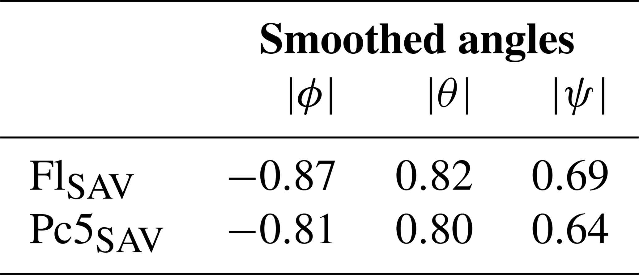
Table 4 Correlation coefficients between functional dependencies of the angles (S(ϕ) and Ak(θ); see text for details) and observational curves (Pc5_SAV and FL_SAV).

4.3 Dates of maxima and minima

To continue the comparison with the three classical hypotheses, we determined the dates of maxima and minima of the SAV in fluence and Pc5 power and compared them with the corresponding dates of maxima and minima predicted by the three hypotheses.

First, we applied a nonlinear least-square fit with five parameters to the superposed median curves (black curves) of Fig. 6. The following function was used:

$$\begin{array}{}\text{(2)}& \begin{array}{rl}f\left(t\right)& =A^{\mathrm{0}}+A^{\mathrm{a}}\sin \left({\displaystyle \frac{\mathrm{2}\mathit{\pi }}{\mathrm{365}}}t+{\mathit{\alpha }}^{\mathrm{a}}\right)\\ & +A^{\mathrm{sa}}\sin \left({\displaystyle \frac{\mathrm{4}\mathit{\pi }}{\mathrm{365}}}t+{\mathit{\alpha }}^{\mathrm{sa}}\right),\end{array}\end{array}$$

with fixed annual and semiannual periodicities and the fitted parameters A⁰, A^a, α^a, A^sa and α^sa. f(t) is plotted in Fig. 10 as a green or red curve in Fig. 10a–b that corresponds to the Pc5 power or fluence fit. The other curves of Fig. 10 are the median and quartiles, as were presented in Fig. 6.

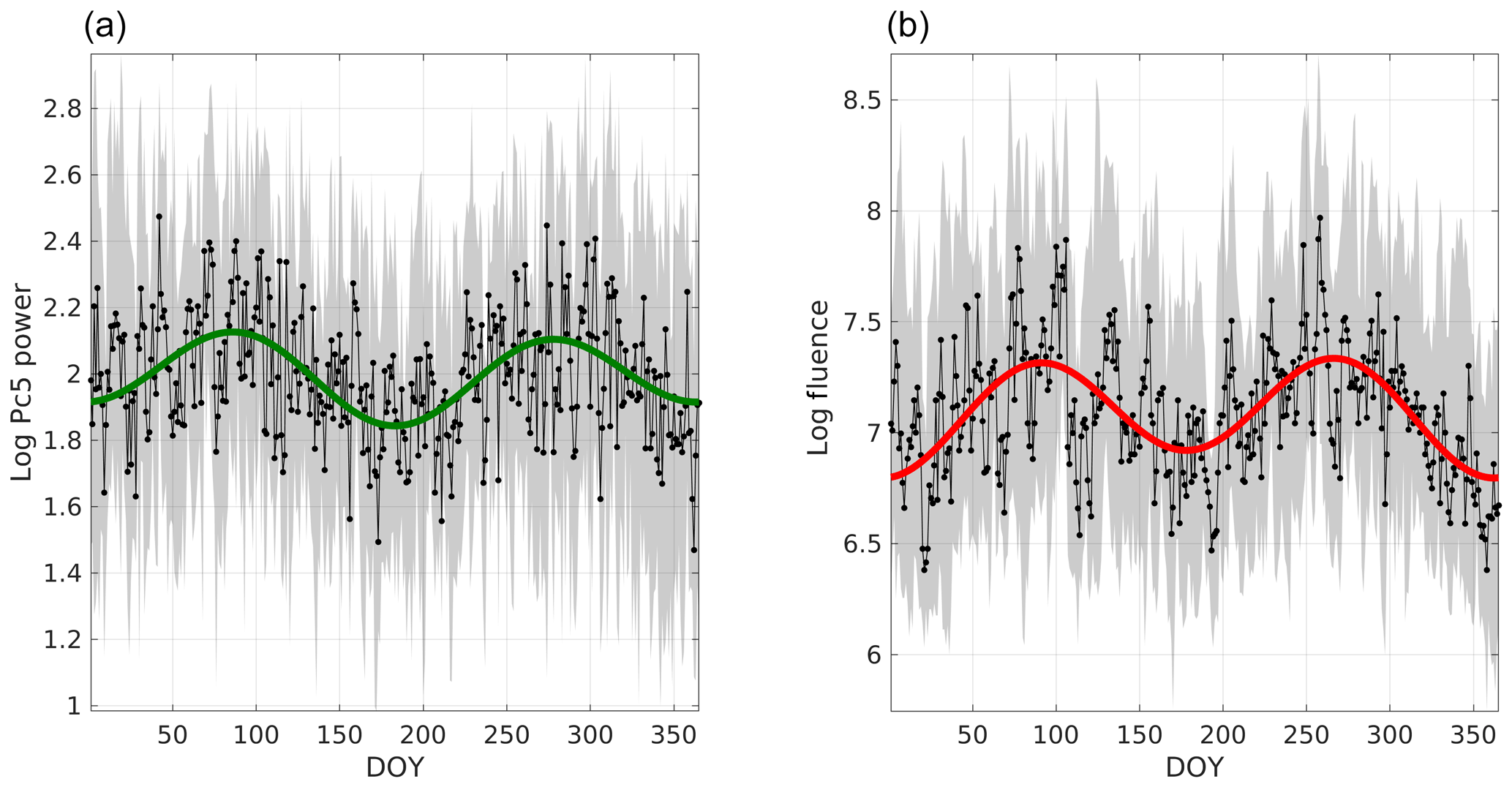
Figure 10 Superposed epoch analysis of the logarithmic daily values of Pc5 power (a) and fluence (b). The median and quartiles are illustrated as a black curve, lower limit and upper limit of the gray band, respectively. The zero epoch is the first DOY. The green and red curves are fits of the median curve, using f(t) as in Eq. (2). The parameters for the fit on the fluence curve are $(A^{\mathrm{0}},A^{\mathrm{a}},{\mathit{\alpha }}^{\mathrm{a}},A^{\mathrm{sa}},{\mathit{\alpha }}^{\mathrm{sa}})=(\mathrm{7.09},-\mathrm{0.06},\mathrm{1.48},-\mathrm{0.23},\mathrm{1.72})$ and for the Pc5 power fit $(A^{\mathrm{0}},A^{\mathrm{a}},{\mathit{\alpha }}^{\mathrm{a}},A^{\mathrm{sa}},{\mathit{\alpha }}^{\mathrm{sa}})=(\mathrm{2},\mathrm{0.04},\mathrm{1.28},-\mathrm{0.12},\mathrm{1.61})$.

Both fits follow the semiannual trend of the superposed median curves very well. In fact, the coefficient that modulates the amplitude of the annual variation is very low for both cases, being $A^{\mathrm{a}}=-\mathrm{0.06}$ for the fluence fit and A^a=0.04 for the Pc5 power fit. But in the semiannual term they are higher, namely $A^{\mathrm{sa}}=-\mathrm{0.23}$ and $A^{\mathrm{sa}}=-\mathrm{0.12}$ for fluence and Pc5 power, respectively. An interesting characteristic that f(t) reveals is that the minima in June and/or July and in December and/or January are not symmetric in both fits. The minimum of f(t) in June and/or July is lower than the minimum in December and/or January for Pc5 power, and the opposite occurs with the fluence fit. On the contrary, f(t) does not present this asymmetry for the maxima in both cases.

Once f(t) was defined, we looked for the t values that obey $\mathrm{d}f\left(t\right)/\mathrm{d}t=f^{\prime }\left(t\right)=\mathrm{0}$, i.e., the times of maxima or minima of f(t) referred to as t_max,min, which will be used as the times of the maxima–minima of the SAV in fluence and Pc5 power. We applied the so-called “Newton–Raphson” method (Ypma, 1995), which is a classic method implemented to find zeros of a function.

We have $f^{\prime }\left(t\right)=\frac{\mathrm{2}\mathit{\pi }}{\mathrm{365}}\left(A^{\mathrm{a}}\cos \left(\frac{\mathrm{2}\mathit{\pi }}{\mathrm{365}}t+{\mathit{\alpha }}^{\mathrm{a}}\right)\right.$ + $\left.\mathrm{2}{A}^{\mathrm{sa}}\cos \left(\frac{\mathrm{4}\mathit{\pi }}{\mathrm{365}}t+{\mathit{\alpha }}^{\mathrm{sa}}\right)\right)$. Expanding f^′(t) up to the linear term around an arbitrary value $\stackrel{\mathrm{̃}}{t}$ near t_max,min and setting $f^{\prime }\left(\stackrel{\mathrm{̃}}{t}\right)\simeq \mathrm{0}$, we find the following:

$$\begin{array}{}\text{(3)}& t\simeq \stackrel{\mathrm{̃}}{t}+{\displaystyle \frac{A^{\mathrm{a}}\cos \left(\frac{\mathrm{2}\mathit{\pi }}{\mathrm{365}}\stackrel{\mathrm{̃}}{t}+{\mathit{\alpha }}^{\mathrm{a}}\right)+\mathrm{2}{A}^{\mathrm{sa}}\cos \left(\frac{\mathrm{4}\mathit{\pi }}{\mathrm{365}}\stackrel{\mathrm{̃}}{t}+{\mathit{\alpha }}^{\mathrm{sa}}\right)}{\frac{\mathrm{2}\mathit{\pi }}{\mathrm{365}}\left(A^{\mathrm{a}}\sin \left(\frac{\mathrm{2}\mathit{\pi }}{\mathrm{365}}\stackrel{\mathrm{̃}}{t}+{\mathit{\alpha }}^{\mathrm{a}}\right)+\mathrm{4}{A}^{\mathrm{sa}}\sin \left(\frac{\mathrm{4}\mathit{\pi }}{\mathrm{365}}\stackrel{\mathrm{̃}}{t}+{\mathit{\alpha }}^{\mathrm{sa}}\right)\right)}}.\end{array}$$

Calling $t=t_{n+\mathrm{1}}$ and $\stackrel{\mathrm{̃}}{t}=t_n$, we iterated Eq. (3) until $|t_n-t_{n+\mathrm{1}}|<{\mathrm{10}}^{-\mathrm{14}}$ d (a cut-off condition for the iteration process), when t_n becomes t_max,min. The dates of the nominal equinoxes and solstices were utilized to initialize the iteration process.

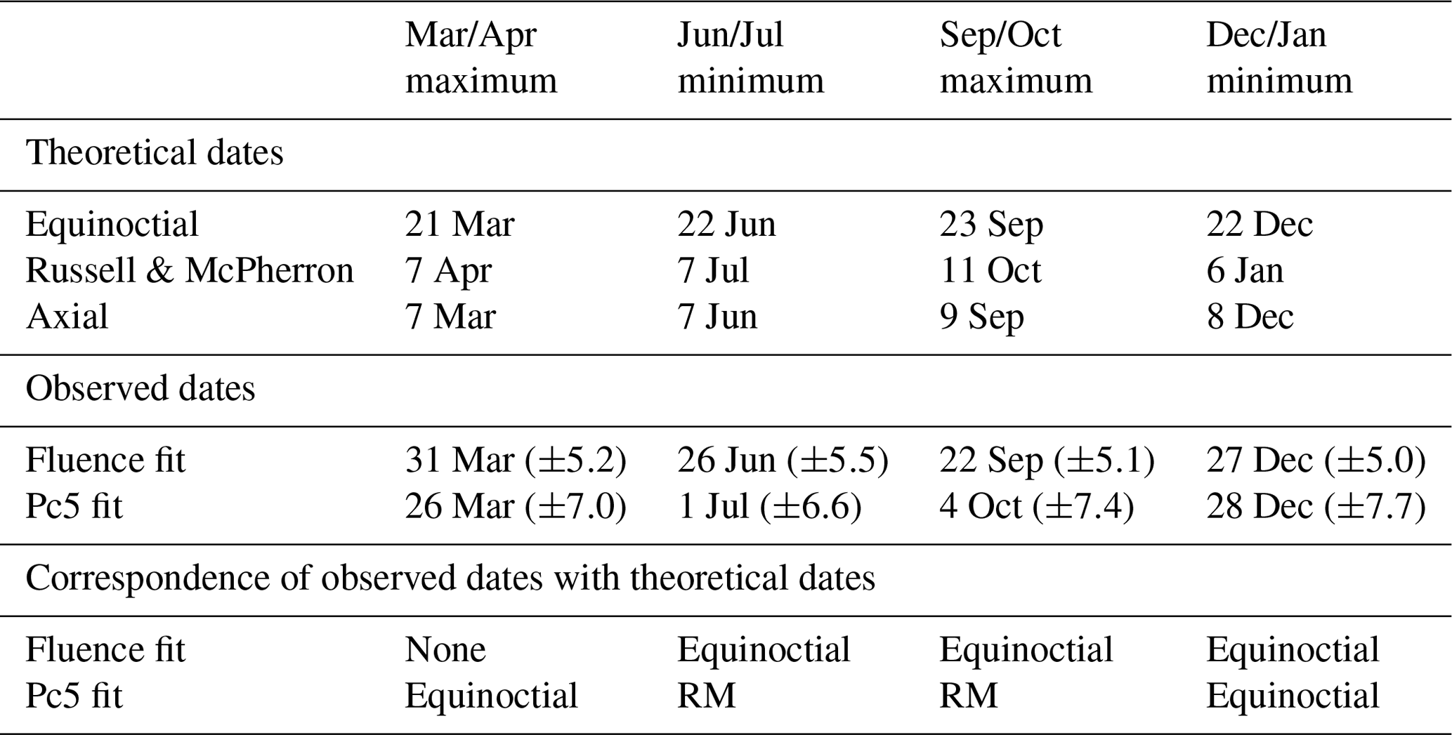
The advantage of calculating t_max,min with this procedure is that Eq. (3) also serves to estimate the errors in the determination of t_max,min because, once t_max,min is determined, we can interpret Eq. (3) as having t expressed as a function of the parameters for values near t_max,min, i.e., $t=F\left(A^{\mathrm{0}},A^{\mathrm{a}},{\mathit{\alpha }}^{\mathrm{a}},A^{\mathrm{sa}},{\mathit{\alpha }}^{\mathrm{sa}}\right)$. Then, error propagation can be used in the determination of t with F. The maxima and minima dates (t_max,min), with their uncertainty interval 2σ_t, are shown in Table 5. The table also shows the dates of maxima and minima predicted by the three mechanisms and which one of them falls into the uncertainty interval.

The best prediction of the SAV minima in fluence is given by the equinoctial hypothesis. This mechanism is also the best one for estimating the September maximum with just 1 d of difference between the observed and predicted date. However, the three mechanisms fail to predict the March maximum in fluence that falls between the equinoctial and RM predictions. Note that if the peak and valley times expected for the equinoctial mechanism are shifted forward 4 d, as in Kanekal et al. (2010), the fluence times of maxima and/or minima fall into the equinoctial uncertainty interval. This time shift was attributed by Li et al. (2001) and Kanekal et al. (2010) to finite solar wind speed (∼440 km s⁻¹).

For the SAV in Pc5 power, it is not possible to find a dominant effect since the RM and the equinoctial theory give the best predictions for one maximum and one minimum but not both.

The results of this section agree with the results found in the profiles analysis of Sect. 4.1. The equinoctial effect seems to be dominant in the generation of the SAV in fluence, and both equinoctial and RM effects might be equally important for the SAV of Pc5 power.

Table 5 Dates of maxima and minima for $\left|\mathit{\varphi }\right|$, $\left|\mathit{\theta }\right|$ and $\left|\mathit{\psi }\right|$ and for the fits (f(t)) of the superposed median curve of Pc5 power and fluence.

5 Discussion

The previous sections have demonstrated a clear SAV in both parameters analyzed in this work. As a result of the length of the observations (two complete SCs of daily values), we were able to recover the background semiannual intensity variation in electron fluence and in Pc5 power. In the first case, this variation can be seen clearly in the red curve of Fig. 6b (Fl_SAV). Fl_SAV reaches ∼7.5 near equinoxes and ∼6.5 near solstices that is equivalent to a difference of 1 order of magnitude, approximately. This means that there is a higher probability of internal charging on satellites near equinoxes, making it more plausible for them to suffer operational anomalies. It also illustrates the way that the SAV influences space-based technologies.

In the study of the dominant effects, we found that the equinoctial mechanism is dominant in the SAV of fluence, and both the equinoctial mechanism and the RM effect play equally relevant roles in the SAV of Pc5 powers. These conclusions are reached by all the correlation values calculated in Sect. 4.1, 4.2 and 4.3 in which the angle profiles of the three mechanisms, functional dependencies of the angles and also the location of maxima and minima dates that the mechanisms predict were analyzed.

These results differ from previous ones reported in Kanekal et al. (2010). Analyzing SAMPEX electron flux data, they found a more prominent role for the RM effect. However, they considered fluxes in the heart of the outer radiation belt (L≃4) to evaluate the leading mechanism and not at the geostationary orbit (GEO). So, it is possible that different mechanisms may control the SAV in relativistic electrons in different regions of the magnetosphere. Another reason why we obtain different results could be that in Kanekal et al. (2010) they used 10 years of daily values (from 1993 to 2002), which are less than half of the measurements processed in this work. Longer time spans of the data make the statistics more representative. In the case of the SAV of Pc5 powers, we were not able to find prior reports studying the controller mechanism to compare with our findings.

The potential of Pc5 power to predict relativistic electron enhancements, combining a set of individual enhancements (Lam, 2017; Georgiou et al., 2018), has been demonstrated before. These events may take place during geomagnetic storms, but they are not exclusively restricted to storm periods, as pointed out in Reeves et al. (2003). In addition to individual enhancements, we have shown that Pc5 power intensity is modulated with a semiannual pattern. This suggests that the SAV in Pc5 pulsations could be the origin of the SAV in relativistic electrons. Nevertheless, additional comprehensive analyses have to be done to confirm this hypothesis. Current works of the authors are being carried out in this direction.

High solar wind speed has been found to correlate well with relativistic electron fluxes enhancements (Paulikas and Blake, 2013). In fact, solar wind speed is used as an input to predict relativistic electron enhancements by means of a linear model (Baker et al., 1990, see https://www.swpc.noaa.gov/products/relativistic-electron-forecast-model, last access: 1 September 2020). However, Reeves et al. (2011) showed that the relationship between the two quantities is more complicated than a linear dependence and established a triangle distribution between them.

An interesting point is that solar wind speed does not show a semiannual pattern. This statement can be probed by calculating an annual superposed curve of solar wind speed, as it is shown in Fig. 4 of McPherron et al. (2009). The superposed solar wind speed curve does not show any regular pattern. This is a strong argument for discarding the axial hypothesis because this hypothesis is based on the variability of solar wind speed throughout the year. Moreover, the lack of a SAV in solar wind speed may be the reason why we obtain the lowest correlation coefficients between the observed curves of this work and the axial hypothesis profile and phases.

Finally, other regular variations have also been studied in this work by means of the ACF calculation. The main periodicities displayed by Pc5 power and fluence were tracked year by year along two complete 11-year SCs, demonstrating that the 27 d period can be observed in every phase of the SC. And this period is most prominent during the declining phase when high correlations at multiples of 27 were also observed. On the contrary, the 27 d period is less recognizable in the ascending and maximum phase.

6 Conclusions

To summarize, this study demonstrates that Pc5 ULF waves and relativistic electrons both vary, with multiple timescales, due to the intrinsic periods of the Sun's dynamics and also those periodicities that result from considering the Sun–Earth system as a whole.

The 11-year solar cycle variation and the 27 d periodicity are associated with the intrinsic periods of the Sun. Enhanced electron levels were found during the declining phase of a solar cycle, as previously reported in other studies. The 27 d periodicity of electrons presented in this study is related to the recurrence of high-speed solar wind streams due to solar rotation.

The semiannual period results from the combination of the periodic dynamic of the Sun and the Earth throughout the year. We have determined the most plausible SAV mechanisms to account for the observations. Similar SAV mechanisms and similar periodicities in both Pc5 power and electrons indicate that Pc5 ULF waves play an important role in energizing electrons, as attested to by other studies.