Lower-thermosphere response to solar activity: an empirical-mode-decomposition analysis of GOCE 2009–2012 data

Forecasting the thermosphere (the atmosphere's uppermost layer, from about 90 to 800 km altitude) is crucial to space-related applications, from space mission design to re-entry operations, space surveillance and more. Thermospheric dynamics is directly linked to the solar dynamics through the solar UV (ultraviolet) input, which is highly variable, and through the solar wind and plasma fluxes impacting Earth's magnetosphere. The solar input is non-periodic and non-stationary, with long-term modulations from the solar rotation and the solar cycle and impulsive components, due to magnetic storms. Proxies of the solar input exist and may be used to forecast the thermosphere, such as the F10.7 radio flux and the Mg II EUV (extreme-ultraviolet) flux. They relate to physical processes of the solar atmosphere. Other indices, such as the Ap geomagnetic index, connect with Earth's geomagnetic environment.

We analyse the proxies' time series comparing them with in situ density data from the ESA (European Space Agency) GOCE (Gravity Field and Steady-State Ocean Circulation Explorer) gravity mission, operational from March 2009 to November 2013, therefore covering the full rising phase of solar cycle 24, exposing the entire dynamic range of the solar input. We use empirical mode decomposition (EMD), an analysis technique appropriate to non-periodic, multi-scale signals. Data are taken at an altitude of 260 km, exceptionally low for a low-Earth-orbit (LEO) satellite, where density variations are the single most important perturbation to satellite dynamics.

We show that the synthesized signal from optimally selected combinations of proxy basis functions, notably Mg II for the solar flux and Ap for the plasma component, shows a very good agreement with thermospheric data obtained by GOCE, during periods of low and medium solar activity. In periods of maximum solar activity, density enhancements are also well represented. The Mg II index proves to be, in general, a better proxy than the F10.7 index for modelling the solar flux because of its specific response to the UV spectrum, whose variations have the largest impact over thermospheric density.

1 Introduction

Forecasting the thermosphere is crucial to space mission design, re-entry operations and space surveillance applications. Most low-Earth-orbit (LEO) operational satellites fly in a narrow zone between 400 and 800 km within this layer. The orbital decay rate of satellites depends on atmospheric drag, which is directly affected by the variable solar activity (Masutti et al., 2016). An orbital decay rate at 250 km of altitude is very significant, causing re-entry of a satellite in about 2 weeks. Large uncertainties in the determination of the satellite impact location during re-entry result from uncertainty of the thermospheric density. During the de-orbiting phase of GOCE (Gravity Field and Steady-State Ocean Circulation Explorer), for instance, 2 h before re-entry, the most probable ground impact area was still extending over the entire descending orbit, across the Pacific and Indian oceans (GOCE Flight Control Team, HSO-OEG, 2014). An impact over Europe could be ruled out just 12 h before satellite disruption.

Various indices and proxies of the solar input are available and used in monitoring and predicting the status of the thermosphere. Most models of atmospheric density have adopted the solar radio flux at 10.7 cm wavelength (the F10.7 index) as a solar flux proxy (Floyd et al., 2005), and the Ap and Kp indices are used for geomagnetic activity (Omniweb, 2018). F10.7 has been measured daily since 1947 at Penticton, Canada, at 17:00, 20:00 and 23:00 UTC. The Ap index instead provides 3-hourly averages of geomagnetic data. Other proxies and indices have been defined over time, some of which are based on direct in situ measurements from satellites and others of which are derived from Earth-based observatories. The Mg II core-to-wing ratio (cwr) has been provided daily since 1978 and is available through the NOAA Space Environment Center or the Institut für Umweltphysik of the Universität Bremen (SORCE, 2018; UVSAT, 2018). The Mg II cwr has proved to be an excellent proxy for the solar mid-ultraviolet (UV) radiation. It originates from a chromospheric line emission near 280 nm. In particular, the chromospheric Mg II H and K lines at 279.56 and 280.27 nm and the weakly varying photospheric wings continuum of the core line emission are observed by a number of on-board satellite instruments. Current semi-empirical models of the thermosphere, such as NRLMSISE-00 (Picone et al., 2002) and JB2008 (Bowman et al., 2008), include satellite drag data, mostly available between 400 and 600 km height, and solar proxies. The NRLMSISE-00 model includes, for instance, the F10.7 solar flux (present and averaged over the previous 81 d) and the Ap index for the previous 57 h. These models, though, may prove inaccurate in predicting neutral thermospheric density, depending on the level of solar activity (see e.g. Lathuillère and Menvielle (2010); Masutti et al. (2016)). During times of high magnetic activity, modelled density may underestimate by a factor of 2 the measured one (Sutton et al., 2005). Moreover, some authors (Pardini et al., 2012) found that below 500 km, many atmospheric models overestimated the average atmospheric density by 7 % to 20 % because of the assumption of a fixed drag coefficient, independent of altitude. An example of how incorrect calculations from empirical models may dramatically affect satellite control is again the case of the GOCE satellite which, soon after launch, went to safe mode because of what proved to be a wrong assumption on density levels. Because of the overestimated drag from model, the satellite attitude was bound to rapidly evolve to a critical tumbling condition, with high risk of loss. Different solar indices may prove more apt than others to reproduce thermospheric density, depending on the status of the solar activity. For instance, the comparison of EUV (extreme-ultraviolet) proxies in thermospheric-density reconstruction at 800 km altitude, from 1997 to 2010 (Dudok de Wit and Bruinsma, 2011), indicated SOHO (Solar and Heliospheric Observatory) EUV data as the most suitable to reproduce thermospheric densities at 800 km, during the analysed period. The Mg II index was also compared to this proxy, showing good, although not optimal, performance, at that altitude.

In our analysis paper, we shall analyse Mg II data available for the 2009–2012 period, thus partly overlapping to that dataset, although at a very different height. We shall use the low-altitude GOCE data which have become available since that cited analysis (Bruinsma et al., 2014).

2 The solar input and thermospheric response

The structure and dynamics of Earth's thermosphere is controlled by the solar input mainly through the highly variable solar EUV radiation, on the day side. Joule dissipation of induced ionospheric currents and kinetic-energy deposition from low-energy particles in the auroral zones (Sarris, 2019; Knipp et al., 2004; Qian and Solomon, 2012) also contribute. Geomagnetic activity, that is particle deposition and ionospheric and magnetospheric effects, is triggered by the interaction with Earth's magnetosphere. The solar wind itself is composed of two components, fast and slow, which may interact with each other during their travel in the interplanetary space, originating shocks impacting Earth's magnetosphere. The EUV flux accounts on average for about 80 % of this energy input, while the geomagnetic input accounts for the remaining 20 %. However, during intense geomagnetic activity, geomagnetic contribution may rise up to about 70 % of the energy input (Immel et al., 2004; Lu et al., 1998). The EUV flux has itself a large (up to a factor of 2) spectrum of variability around its base value (Del Zanna and Andretta, 2011). Thus geomagnetic activity is a variable source of energy and has an impulsive component varying on short timescales of hours, during geomagnetic storms, and a more stable background, away from storms. These fast variations in time, may cause local variation of density of a factor of 2 or 3 with respect to the pre-event average value (see Fig. 4 below). Radiative input from the Sun, instead, has a more continuous character. The 27 d solar rotation period induces changes in the solar emission correlated with the motion of active regions across the Earth-facing solar disk. During the course of the 11-year solar cycle, density is seen to vary by a factor of about 6 at low altitudes (250 km). Seasonal and semi-annual variations are induced by the movement of the sub-solar point and the uneven heating of the two hemispheres at solstices. Diurnal variations are also present, which produce an asymmetry in density between the Sun-lit and the dark hemispheres. Thermosphere thus responds to this composite input on many different timescales.

3 Data sets: GOCE thermospheric-density and solar and geomagnetic indices

GOCE, the Gravity Field and Steady-State Ocean Circulation Explorer (Drinkwater et al., 2003), was launched by ESA (European Space Agency) on 17 March 2009 to map Earth's gravity field. It has had a 5-year lifetime, flying at the exceptionally low altitude of between 260 and 230 km. No other civilian satellite has ever flown this low within the thermosphere for such an extended time. GOCE was kept in a drag-free orbit in a dawn–dusk 96.7^∘ Sun-synchronous orbit. The mission profile is shown in Fig. 1. As apparent from the figure, soon after commissioning, GOCE was brought to a mean altitude of 260 km. Nominal operations then started in September 2009, going on through the end of July 2012. On 1 August 2012, after 3 years flying at its nominal altitude, a low-orbit campaign was started for GOCE, steadily bringing its orbit down to 229 km. De-orbiting then started on 20 October 2013, and the satellite was lost few days later. Figure 2 shows the full span of the GOCE thermospheric-density dataset in the context of solar cycle 24. The red boxes show how the GOCE mission covers the full rising phase from the solar minimum to the solar maximum. Within the GOCE mission time, three sub-periods have been identified and selected for subsequent analysis: a phase of low solar activity, from mission start to the end of September 2010; a rising phase, until July 2012, where activity rises from its minimum to maximum level; and a phase of steady, high activity until the end of the mission in November 2013, where activity is almost stationary and close to solar-maximum levels. Compared with the mission profile timeline, the period of high activity coincides with GOCE's low-orbit campaign. The average value of density is therefore expected to be monotonously rising with time, in this period, due to altitude lowering. The level of solar activity is, instead, stationary at the highest levels. Decoupling of the trend due to orbit lowering is therefore possible in density data from this last period.

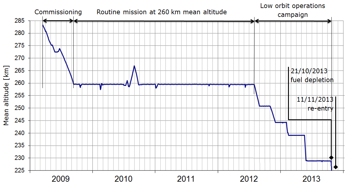
Figure 1 GOCE mission profile (GOCE Flight Control Team, HSO-OEG, 2014). Low-orbit campaign (260–230 km height) starts on 1 August 2012 and goes through until the end of the mission on 20 October 2013.

To keep the satellite in the drag-free mode, extremely sensitive accelerometers were coupled to an ion thruster. Data from the accelerometers have been processed to a thermospheric-density dataset (Bruinsma et al., 2014) which has been made available by ESA through the GOCE Virtual Archive (ESA, 2016). Data are organized in monthly data files starting on 1 November 2009 00:00:00 and ending on 20 October 2013 04:07:10. The sampling rate is 10 s. We use release 1.5 of the dataset. Data for the geomagnetic Ap index and solar index F10.7 have been retrieved from the NASA Goddard Space Flight Center OMNIWeb interface (Omniweb, 2018). The composite Mg II index v5 dataset was retrieved from UVSAT (Ultraviolet Satellite Data and Science Group) of the Institut für Umweltphysik of the Universität Bremen (UVSAT, 2018). The sunspot number was retrieved from SILSO (Sunspot Index and Long-term Solar Observations) data and the image portal of the Royal Observatory of Belgium, Brussels.

In the subsequent analysis, solar proxies are tested with their capability to reproduce thermospheric density, within these three different dynamical regimes.

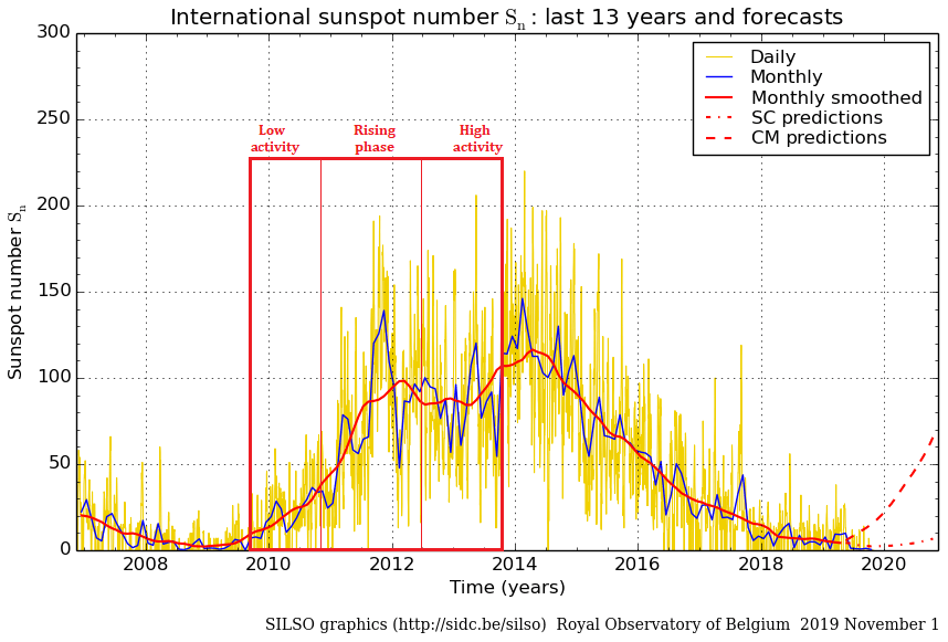
Figure 2 GOCE dataset in the context of solar cycle 24. The inset shows the data span, further divided into low activity (from mission start), medium activity (rising phase of solar cycle 24, from 24 September 2010) and high activity (solar cycle 24 stationary phase of high activity, from 4 July 2012), which mostly coincides with the altitude-lowering phase of the mission, starting 1 August 2012.

In Fig. 3, the whole-mission thermospheric-density dataset is shown. The density signal is sampled at 10 s and has a periodic, high-frequency component due to the satellite orbit, lasting 90 min. We remove this high-frequency component, shown in the inset of Fig. 3, by averaging the signal over 1 d, that is approximately 16 orbits. Due to in-flight anomalies, the density dataset is affected by gaps, ranging from tens of seconds to days. The most significant gap starts on 8 July 2010 and lasts 67 d. Also to be noted is the expected steady increase in average density due to the orbit lowering after July 2012. The signals from solar and geomagnetic proxies, F10.7, Mg II and Ap, have been pre-treated for outlier identification and removal. Spline interpolation has been used to fill in missing or removed data. The Ap signal, which is available on a 3 h interval, has been averaged over 24 h. The Ap index has also been shifted by a fixed 9 h amount. The thermosphere, in fact, reacts to the impulsive geomagnetic forcing with a delay. We have determined this delay by maximizing the correlation between Ap and ρ signals during geomagnetic events, resulting in a fixed 9 h delay, which has been applied to the Ap signal. Geomagnetic storms represent the impulsive component of the solar input, lasting from hours to days. They originate from solar plasma ejected during CME (coronal-mass-ejection) events which impacting Earth's magnetosphere or from shocks forming at the interfaces between fast and slow solar wind. Figure 4 shows four examples of atmospheric response to geomagnetic storms, which occurred during mission lifetime and are captured by GOCE. Reconfiguration of the geomagnetic field induces currents in the ionosphere. Remembering that the sample period for Ap is 3 h, thermospheric response to geomagnetic forcing may indeed be between 6 and 12 h. Figure 4 also shows (see e.g. top left panel) how thermospheric response is not only delayed but relaxes to the quiet state with a finite characteristic time of the order of 1 d. Thus, a second event happening during relaxation (see e.g. bottom left panel) will add to the first one, not yet relaxed, resulting in an enhanced value of the thermospheric density (see e.g. panel b). This memory effect is not included in our model, which only considers a mean time lag between storms and thermospheric-density enhancement. A dynamical model may be constructed, also accounting for relaxation (see e.g. Dudok de Wit and Bruinsma, 2011), which may better fit multiple impulsive events, thus being more characteristic of phases of high solar activity, close to the solar maximum.

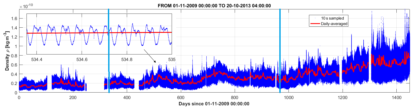
Figure 3 Thermospheric density from GOCE data. Density profile, provided at a 10 s sampling rate (blue line), is averaged over 1 d (red line). In the inset sub-plot, a time span of only 10 orbits is plotted. The periodic, high-frequency fluctuations of density are due to satellite orbit, lasting around 90 min. In the main plot, day 0 is the start of operations (1 November 2009). Blue vertical lines at day 327 (24 September 2010) and 976 (4 July 2012) indicate the limits of the three sub-datasets of low, rising and high solar activity (see also Fig. 2). Low-orbit campaign starts on day 1004 (1 August 2012), almost completely overlapping with the low-orbit campaign. The RSS (root sum of squares) error in density (not shown) is also provided in the dataset, setting a level 2 orders of magnitudes lower than the average density.

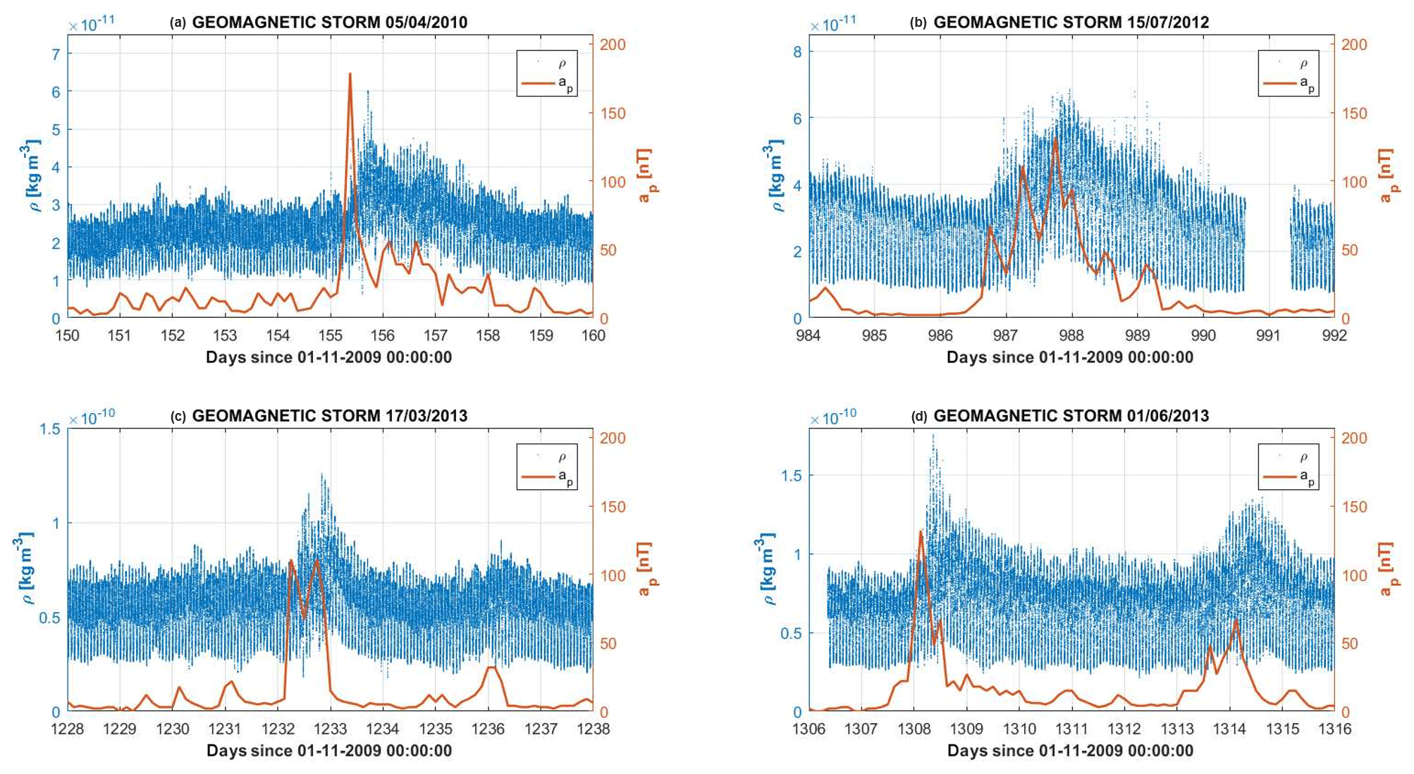
Figure 4 Thermospheric-density ρ (blue line) and Ap index (red line) during four geomagnetic storms occurred over the course of the GOCE mission: (a) 5 April 2010 (day 155), (b) 14 July 2012 (day 986), (c) 13 March 2013 (day 1232), and (d) 1 and 7 June 2013 (days 1308 and 1314).

Figure 5 shows the evolution of whole-mission thermospheric density, together with that of solar indices Ap, F10.7 and Mg II. It is apparent from the figure that the geomagnetic index Ap does not capture the overall trend due to the rising solar cycle, describing only impulsive events. Mg II and F10.7 better follow the long-term trend of thermospheric density. Both F10.7 and Mg II over-represent modulations due to solar rotation (see e.g. the main modulation during days 800 to 1000) than thermospheric density. Correlation, though, is apparent. As expected, a very poor average correlation is shown by ρ and Ap, due to the intermittent nature of the geomagnetic input. Correlation between ρ and solar fluxes is instead clear, being higher in times of low solar activity, which is for low values of F10.7 and Mg II. In times of high solar activity (high values of F10.7 and Mg II), the correlation with solar fluxes gets worse. Mg II tends to be better correlated than F10.7 at average values of thermospheric density, confirming the role of UV flux in coupling with the thermosphere. A correlation coefficient of

$$\begin{array}{}\text{(1)}& R_{xy}={\displaystyle \frac{{\mathit{\sigma }}_{xy}}{{\mathit{\sigma }}_x{\mathit{\sigma }}_y}}\end{array}$$

may be calculated between the variables ρ, F10.7 and Mg II, resulting in values of $R_{\mathit{\rho },\mathrm{F}\mathrm{10.7}}=\mathrm{0.57}$ and $R_{\mathit{\rho },\mathrm{Mg}\mathrm{II}}=\mathrm{0.67}$, respectively, indicating a better overall correlation between the thermospheric-density and Mg II index, with respect to F10.7. EMD (empirical-mode-decomposition) analysis below will further clarify the interplay of the various indices to reproduce the density fluctuations.

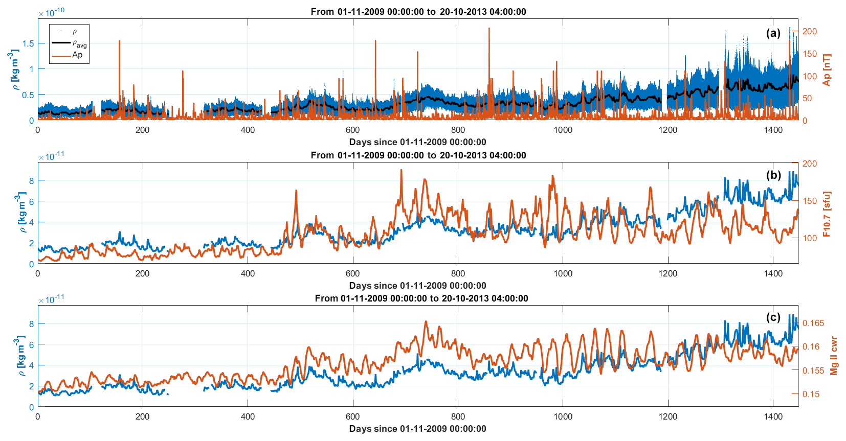
Figure 5 Comparison of time series for whole-mission thermospheric-density and solar indices Ap, F10.7 and Mg II. (a) Density (full dataset, blue line; daily averaged, black line) with the Ap index (red line). (b, c) Daily averaged density (blue) and F10.7 and Mg II indices (red), respectively. Solar flux unit: sfu.

4 Data analysis and density synthesis from proxies

Time series from the solar proxies result from non-stationary and non-linear problems. Standard signal-processing analysis tools such as harmonic decomposition or wavelet analysis are not suited to extract relevant features from Sun-related time series (Lovric et al., 2017). Empirical mode decomposition (EMD) (Huang et al., 1998) will be used for analysing all time series in this paper. EMD decomposes a signal as the sum of a finite number of basis functions called intrinsic mode functions (IMFs). These are generated iteratively by constructing successive envelopes of the signal and then removing this envelope and iterating. This process returns global modes (as opposed to wavelets which are local modes) which are non-periodic (as opposed to Fourier base functions) and with almost zero mean value. IMFs are representative of trends embedded in the signal with a time-variable amplitude and frequency yet still characterized by a typical scale length. The lowest modes are associated with the highest temporal variability. The highest mode is the global trend. IMFs are given in the time domain and are defined in the full time domain as the original dataset. The algorithm defining the IMF technically consists in a series of steps (called sifting), whereby all local extrema (minima and maxima) of a signal x(t) are identified; local minima are then interpolated by cubic spline to get a lower envelope e_min(t). A similar procedure on maxima defines an upper envelope e_max(t). A mean envelope $m\left(t\right)=\left[e_{min}\right(t)+e_{max}(t\left)\right]/\mathrm{2}$ is then calculated, returning the low-frequency part of the original signal x(t). This process is iterated, starting from a new signal obtained by removing the mean envelope m(t) from the original signal $h\left(t\right)=x\left(t\right)-m\left(t\right)$. In this way, a set of IMFs containing the highest-frequency features is obtained first. Iteration is than carried out, defining more IMFs, until the residual between signal and the IMF become a monotonic function from which no further IMF can be extracted. Figures 7–9 show the full set of IMFs in the EMD decomposition for solar proxies' time series.

5 Results

Solar proxies are analysed, and the resulting set of IMFs are reported in Figs. 7–9. The lowest-order IMFs are associated with the most rapidly varying components of the signal, while the residual captures the overall trend. The number of IMFs is not fixed a priori and depends on the convergence criterion chosen for stopping the EMD algorithm.

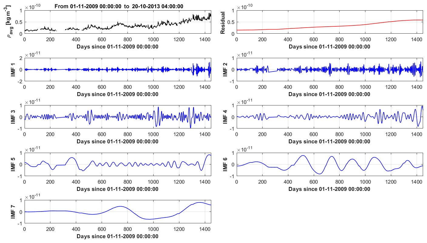
Figure 6 EMD decomposition for the thermospheric-density signal from the GOCE data, 2009–2013. Top row: original signal and trend. From first row: successive orders of basis functions (IMFs).

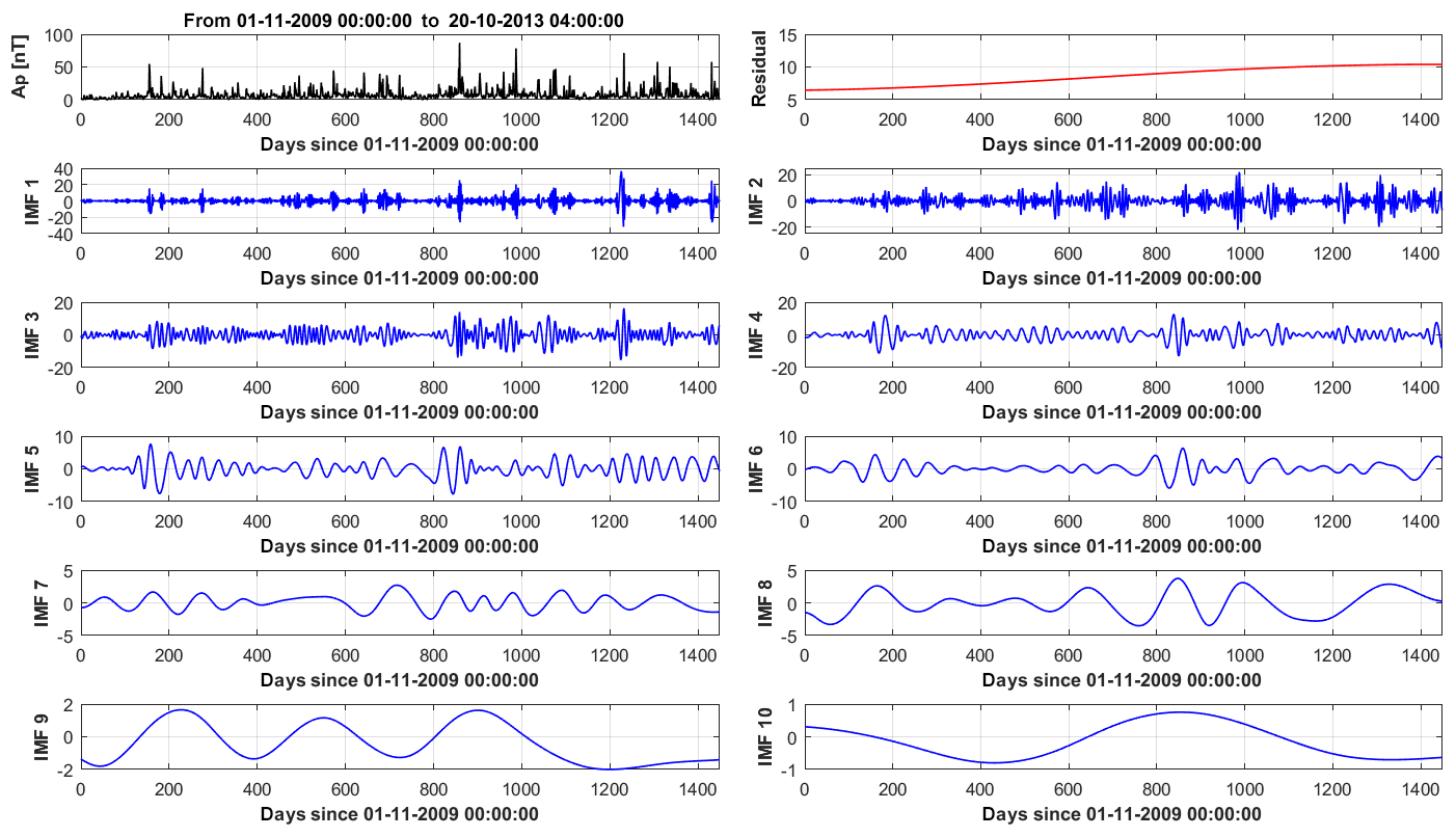
Figure 7 EMD decomposition for the geomagnetic index Ap. Top row: original signal and trend. From first row: successive orders of basis functions (IMFs).

Figure 8 EMD decomposition for the F10.7 solar radio flux. Top row: original signal and trend. From first row: successive orders of basis functions (IMFs). Solar flux unit: sfu.

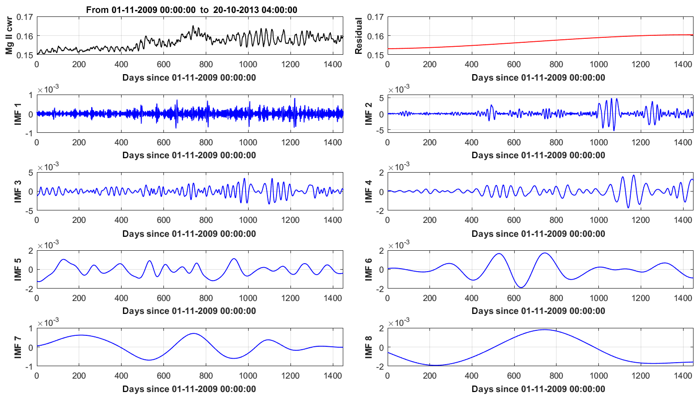
Figure 9 EMD decomposition for the Mg II solar UV flux proxy. Top row: original signal and trend. From first row: successive orders of basis functions (IMFs).

The thermospheric-density signal is then reconstructed from a linear superposition of the set of IMFs from the solar proxies:

$$\begin{array}{}\text{(2)}& \begin{array}{rl}\overline{\mathit{\rho }}& =N[A^{\mathrm{Ap}}\cdot \sum _i{c}_i^{\mathrm{Ap}}{\mathrm{IMF}}_i^{\mathrm{Ap}}+A^{F_{\mathrm{1}}\mathrm{0.7}}\cdot \sum _i{c}_i^{F\mathrm{10.7}}{\mathrm{IMF}}_i^{F_{\mathrm{1}}\mathrm{0.7}}\\ & +A^{\mathrm{Mg}\mathrm{II}}\cdot \sum _i{c}_i^{\mathrm{Mg}\mathrm{II}}{\mathrm{IMF}}_i^{\mathrm{Mg}\mathrm{II}}],\end{array}\end{array}$$

where the coefficients c_i may be zero or one, thereby selecting only a subset of the IMF component functions resulting from the signal analysis. We have determined the optimal combination of IMFs, capable of reproducing the signal, based on the minimization of the RMSE (root mean square error):

$${\mathit{\sigma }}_{\mathrm{RMS}}=\sqrt{{\displaystyle \frac{\mathrm{1}}{N}}\sum _{i=\mathrm{1}}^N(\mathit{\rho }-\overline{\mathit{\rho }}}{)}^{\mathrm{2}}.$$

Figure 10 shows the best synthesized signal from a combination of the whole-mission IMF modes from Ap, Mg II and F10.7. Figure 11 shows instead the best synthesized signals from the different sets of IMFs determined for the three separate subsets, during the phase of low solar activity, rising phase and the phase of high solar activity. Table 1 shows, for all cases, the individual components of the optimal synthesized signal. Table 2 compares the optimal solution with two cases where either F10.7 or Mg II is selected as the solar UV proxy. A number of considerations may be drawn from the analysis. Firstly, all syntheses require the Ap signal to be taken into account, although during low solar activity its amplitude and therefore its relative contribution to the overall signal is small. This confirms the relevance of the state of the interplanetary medium on the short-term dynamics of the thermosphere. The Ap signal is intermittent, and all IMF components are always needed to reconstruct the signal. This is not the case for the solar flux proxies F10.7 and Mg II, whose long-wavelength components appear most in the decomposition for all periods. The solar input is therefore basically captured on the short timescale by the variations of the geomagnetic input captured by Ap and on the longer timescales by the proxies of the solar radiative flux F10.7 and Mg II. During the rising phase of the solar cycle and during the period of high solar activity, the contribution of the geomagnetic proxy Ap has a much higher amplitude than during low activity, and the contribution to the density of changes in the interplanetary medium is therefore dynamically relevant. Another conclusion which can be drawn is that the Mg II index performs better than the F10.7 index. In fact, the sole combination of Ap and Mg II performs very similarly to the full combination of the three indices. The only exception is for periods of low solar activity, where inclusion of F10.7 somewhat improves signal reconstruction.

We have seen earlier how low-orbit operations overlap with the period of high solar activity. A rising trend in average density is therefore apparent in Fig. 10, due to density increase because of orbit lowering. This rising trend could not be captured by the solar indices in the same figure. However, if de-trended, in the third period data are shown as in Fig. 12, where the rising trend is no more seen and an agreement of the two curves is on the same level as in the previous period of rising solar activity. Table 1 reports the values of the RMSE in the period of high activity for the original and the de-trended density signal, showing a decrease from 14 % to 11 % when accounting for a density increase due to orbit lowering.

Table 1 Components of optimal synthesized signal for the whole mission and low, rising and high solar activity during solar cycle 24. RMSE σ_RMS (normalized to the mean value) and component amplitudes A.

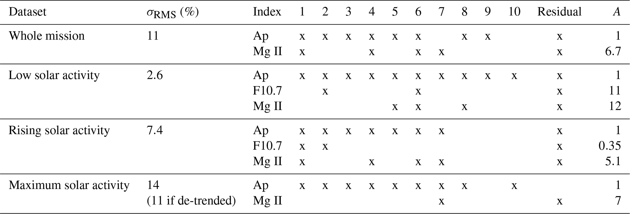
Table 2 Comparison of normalized RMSE values (in %) for different optimal combinations of proxies.

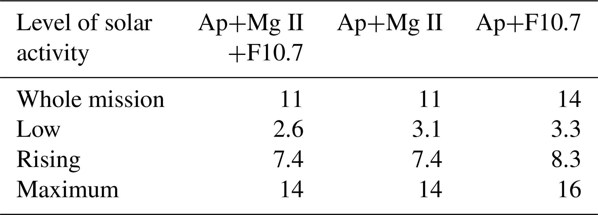
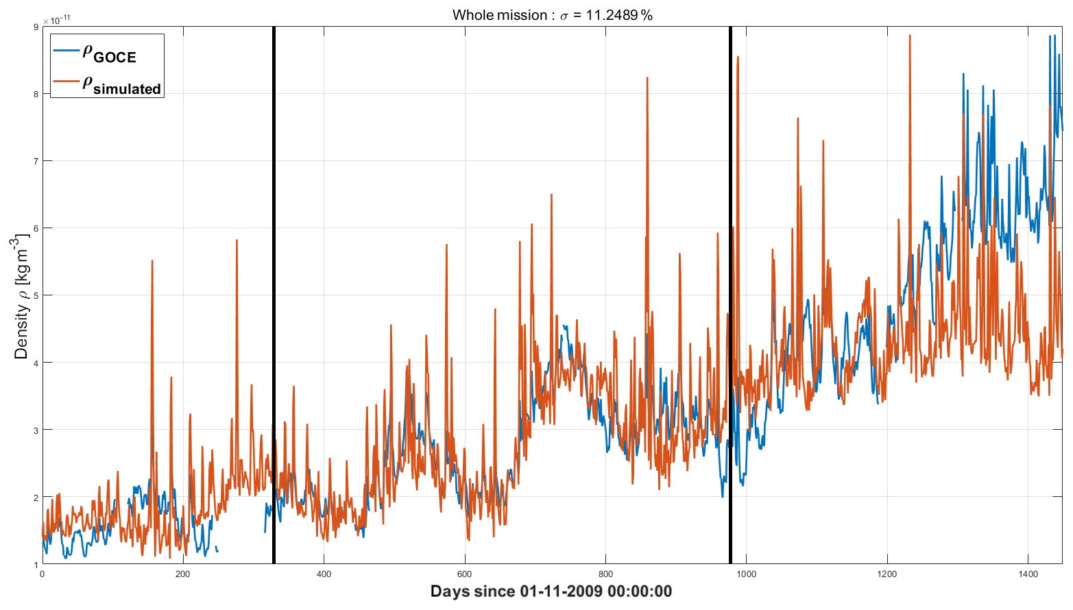
Figure 10 Thermospheric density synthesized (red line) from the optimal combination of Ap, Mg II and F10.7. Whole mission. Blue line shows thermospheric-density data. The rising trend in density in the last third of the mission is due to orbit lowering and is therefore not shown in the reconstructed signal.

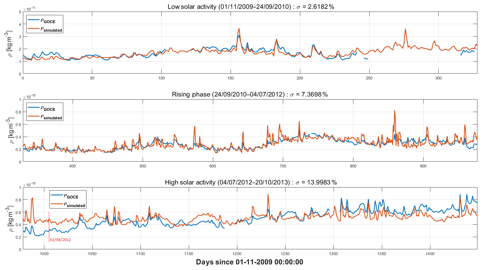
Figure 11 Optimal synthesized thermospheric density from Ap, Mg II and F10.7. Three different EMD sets for the extent of the whole mission, each covering one of the three selected dynamical activity regimes for solar cycle 24, low, rising and high. The trend in density apparent in the phase of high solar activity is due to orbit lowering and is therefore not shown in the reconstructed signal.

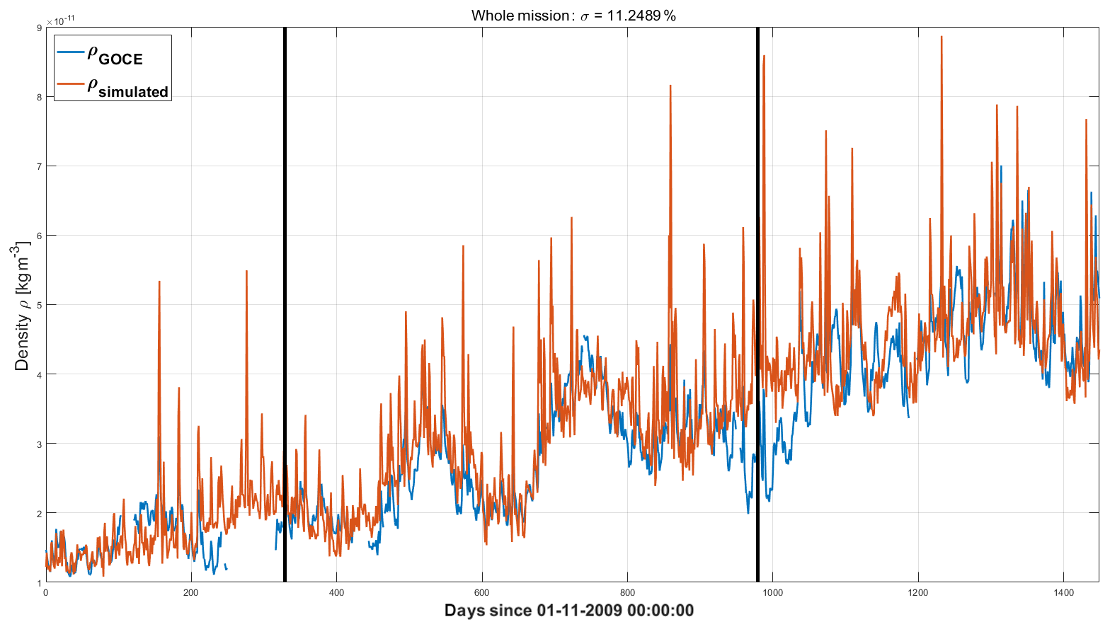
Figure 12 Effect of orbit lowering on the third period of high solar activity, from 1 August 2012. Density data (blue line), as shown in Fig. 10, have been de-trended to subtract the contribution due to orbit lowering. Red line shows synthesized thermospheric-density values from the optimal combination of Ap, Mg II and F10.7. Whole mission.

6 Conclusions

We have performed an analysis of three of the most commonly used solar flux and geomagnetic proxies, F10.7, Mg II and Ap in relation to the time evolution of thermospheric density measured in situ from 260 to 230 km altitude, using the GOCE thermospheric-density dataset, which spans most of the rising phase of solar cycle 24, from minimum to maximum, covering the full dynamical spectrum of the solar input of the thermosphere. The thermospheric-density signal, for the whole mission and from three sub-intervals of low, rising and high solar activity, has been analysed through empirical mode decomposition. Once the basis functions have been determined, they have been optimally recombined to reconstruct the density signal. Analysis shows how the geomagnetic proxy Ap is always needed to capture the impulsive short-term features of the density signal connected with the evolution of the interplanetary medium. However, during low solar activity, Ap contribution has a much lower amplitude than the other signals. The thermospheric density in this period is therefore driven by the low-frequency variations of the radiative input, captured by the solar flux proxies F10.7 and Mg II. A lesser contribution comes from the drive of the interplanetary medium impacting Earth. During the rising phase of the solar cycle and during the period of high solar activity, the contribution of the geomagnetic proxy Ap has a much higher amplitude than during the period of low activity, and the contribution to density of changes in the interplanetary medium is therefore dynamically relevant. During low and medium solar activity, the thermospheric signal can be reconstructed with RMSE values of about 2.6 % and 7.4 %, respectively. Semi-empirical atmospheric models (NRLMSISE-00 and Jacchia family models above all) are usually credited to fall in the 10 % error range. During high solar activity, error increases to 14 %, but this figure is worsened by the steady rising trend in mean density due to orbit lowering, not present in the solar input, and is therefore over-estimated. If de-trended, the signal shows an root mean square value, in the third period, of 11 %. The selection of the optimal combinations, which we have presented in this paper, is instead independent on the absolute value of Mg II, which proves to be a better proxy than F10.7 in capturing the long-term trends of the solar input during the solar cycle and is therefore to be preferred if only the long-term trend is of interest. Combining Ap (shifted by 6 h to take into account the thermosphere's dynamical response to the solar input) and the slowest-varying EMD modes from Mg II returns a good representation of the thermospheric-density signal at low thermospheric altitudes. A final comment should be addressed to the forecasting capability of the reconstruction of density from solar proxies for different altitudes. The thermospheric-density changes by orders of magnitude between 250 and 800 km, that is the portion of our thermosphere where most LEO satellites fly. In this paper we have followed the long-term evolution of density at 260 km, rising by almost 1 order of magnitude through the solar cycle. Extrapolating our results to 800 km altitude would need a self-consistent thermospheric model at different altitudes which is not yet established. On the other hand, constraining current models with datasets at different heights seems to be necessary step, and the GOCE dataset may be instrumental in such a programme.