Performance of the IRI-2016 over Santa Maria, a Brazilian low-latitude station located in the central region of the South American Magnetic Anomaly (SAMA)

In this work we analyze the ionograms obtained by the recent digisonde installed in Santa Maria (29.7^∘ S, 53.7^∘ W, dip angle = −37^∘), Brazil, to calculate the monthly averages of the F2 layer critical frequency (foF2), its peak height (hmF2), and the E-region critical frequency (foE) acquired during geomagnetically quiet days from September 2017 to August 2018. The monthly averages are compared to the 2016 version of the International Reference Ionosphere (IRI) model predictions in order to study its performance close to the center of the South America Magnetic Anomaly (SAMA), which is a region particularly important for high-frequency (HF) ground-to-satellite navigation signals. The foF2 estimated with the Consultative Committee International Radio (CCIR) and International Union of Radio Science (URSI) options makes good predictions throughout the year, whereas, for hmF2, it is recommended to use the SHU-2015 option instead of the other available options (AMTB2013 and BSE-1979). The IRI-2016 model outputs for foE and the observations presented very good agreement.

1 Introduction

The growing importance of space technologies through satellites for a large variety of applications such as science, Earth observation, meteorology, communications, security, and defense puts forward the need to improve our ability of ionospheric modeling. For instance, the drag force on satellites in low-Earth orbit (LEO, generally defined as an orbit below an altitude of approximately 2000 km) increases when the solar activity is at its greatest over the 11-year solar cycle, which may cause uncontrolled re-entry and degrade the predictions of satellite positions (Horne et al., 2013). During space weather conditions as defined by Denardini et al. (2016), elevated flux levels of high energetic particles may precipitate in the ionosphere in regions of anomalously weak geomagnetic field strength such as the South America Magnetic Anomaly (SAMA). Besides enhancing the ionization distribution and conductivities (Moro et al., 2012, 2013), the energetic particles create high background counts which render satellite sensors unusable in this region (Schuch et al., 2019; Heirtzler, 2002). Operators who control satellites in LEO may need to know with a high degree of accuracy when and where to turn satellites on and off to minimize the risk of detector saturation (Jones et al., 2017). Ionospheric modeling is also important for ground assets since it is essential to predict the ionospheric behavior for successful radio communication. Since drastic ionospheric variations can affect the performance of radio-based systems, such prediction may identify the periods, the path regions, and the sections of high-frequency bands that will allow or disrupt the use of the radio transmissions (Ezquer et al., 2008).

One of the most widely used ionospheric models is the International Reference Ionosphere (IRI), which became the official International Standardization Organization (ISO) standard for the ionosphere in April 2014 (Bilitza et al., 2017). IRI is a joint project of the Committee on Space Research (COSPAR) and International Union of Space Science (URSI). It is derived from ionospheric observations collected by ground and in situ measurements such as the worldwide network of ionosondes, incoherent scatter radars, several compilations of rocket measurements, and satellite data. The model describes monthly averages of the electron density, electron and ion temperature, total electron content (TEC), and ion composition as a function of height, location, and local time. Several major milestone editions of IRI have been released by the IRI Working Group since the 1970s in order to constantly revise the model to keep it as up to date and accurate as possible (Rawer et al., 1978a, b, 1981; Bilitza, 1990, 2001; Bilitza and Rawer, 1996; Bilitza and Reinisch, 2008; Bilitza et al., 2014, 2017). The latest version is known as IRI-2016 and has important improvements over the 2012 and 2007 versions (IRI-2012 and IRI-2007, respectively). The most important update is the inclusion of two new model options for the F2 layer peak height, hmF2. These two options allow the users to model the hmF2 directly and no longer depend on the propagation factor M3000F2 described by Bilitza et al. (1979). Besides, IRI-2016 has a better representation of topside ion densities during very low and high solar activities. The details about the IRI model are available on the following home page: http://irimodel.org/ (last access: 12 August 2019).

Among several parameters, IRI can predict the F2 layer critical frequency (foF2), hmF2, and the E-region critical frequency (foE) for a given time and location. The correct understanding of these parameters is particularly important for space technologies. The critical frequencies are two key parameters when calculating the electron densities of the ionosphere at F2 (NmF2) and E-region heights. Moreover, foF2 is related to the maximum usable frequency for the radio waves reflection and TEC that is significant for the phase delay of high-frequency (HF) ground-to-satellite navigation signals (Fuller-Rowell et al., 2000). On the other hand, hmF2 receives much of the attention since it gives the highest stratification of the upper ionosphere.

In the literature, several papers have reported many comparative studies around the globe between the ionospheric parameters measured by ionosondes and different versions of the IRI to study its performance. In South America, Ezquer et al. (2008) analyzed NmF2 over Tucumán (26.9^∘ S, 66.4^∘ W, dip angle = −26^∘), Argentina, during the low and high solar activity years 1965 and 1970, respectively, and the moderate solar activity years 1967 and 1972. Bertoni et al. (2006) used foF2 and hmF2 measured by two digital ionosondes installed at two Brazilian low-latitude stations in July 2003, October 2003, January 2004, and April 2004. They compared the data collected in Palmas (10.1^∘ S, 48.2^∘ W, dip angle = −12^∘) and São José dos Campos (23.2^∘ S, 45.8^∘ W, dip angle = −33^∘) with the IRI-2001 predictions. Batista and Abdu (2004) compared the parameters foF2, hmF2, and B₀ measured by two digital ionosondes over São Luís (2.6^∘ S, 44.2^∘ W, dip angle = −4.3^∘, magnetic equator) and Cachoeira Paulista (22.7^∘ S, 45^∘ W, dip angle = −33.5^∘, close to the southern crest of the equatorial ionization anomaly – EIA) with the IRI-2007 for high and low solar activity periods. Moro et al. (2016) tested the influence of IRI-2007 in deriving the conductivity profiles and electric files in the Brazilian equatorial region. In Africa, Oyekola and Fagundes (2012) compared foF2, hmF2, and propagation factor (M3000F2) recorded near the dip-equator in Ouagadougou, Burkina Faso (12^∘ N, 1.8^∘ W; dip angle = 2.9^∘) with IRI-2007 during low (1987) and high (1990) solar activity, and undisturbed conditions for four different seasons. In Europe, Maltseva and Poltavsky (2009) investigated several aspects of the IRI accuracy and efficiency for long-term prediction of the foF2 and the maximum usable frequencies (MUF) using the storm-time correction option, TEC, and the maximum observable frequency (MOF) for the year 2005. In China, Zhao et al. (2017) used hmF2 data derived by ionosondes at Mohe, Beijing, Wuhan, and Sanya from 2007 to 2016 to assess the performance of the three options for the IRI hmF2, while Liu et al. (2019) used foF2 measured over four stations in China (covering from 49.4 to 23.2^∘ N) from January 2008 to October 2016 to test IRI foF2. The aforementioned studies show that the ionospheric parameters predicted by the IRI model differed from the ionosonde data at a different location. Generally, IRI overestimates the ionospheric parameters at the magnetic equator and underestimates at EIA crests.

The aim of this work is to use the critical frequencies foF2 and foE and the height hmF2 measured by a recent 4D digisonde portable sounder (DPS-4D) installed in Santa Maria (29^∘ S, 54^∘ W, dip angle = −37^∘), Brazil, to test the performance of the IRI-2016 in the low-latitude ionosphere situated close to the center of the SAMA. The Santa Maria digisonde (SMK29) is supported by the Space Weather Monitoring Meridian Project of China (Wang, 2010), the Brazilian Study and Monitoring of Space Weather (Embrace) Program from the Brazilian National Institute for Space Research (INPE/MCTIC), and the Federal University of Santa Maria (UFSM). Notice that there are very few ionospheric sounders operating in real-time in the low- and mid-latitudes in South America, and SMK29 fills a gap of ionospheric sounding between Cachoeira Paulista station and Port Stanley station (51.6^∘ S, 57.9^∘ W, dip angle = −49.8^∘), Argentina. Therefore, validating the IRI-2016 in a region under the influence of the SAMA is particularly important for HF communication and radio-based space systems as described before, as is the contribution of the IRI Working Group in evaluating the efficacy of the model in the low-latitude Brazilian region.

2 Observed data, modeling, and method of analysis

The SMK29 is set to transmit radio waves continuously into the ionosphere from 1 MHz and increases the frequency up to 20 MHz with the sweep rate of 25 kHz for each round. The train of echoes to form an ionogram is transmitted and received with a 5 min temporal resolution. All recorded ionograms are initially auto-scaled by the Automatic Real-Time Ionogram Scaler with True Height (ARTIST). Then, the observed foF2, foE, and hmF2 parameters are deduced from manually scaled ionograms with help of the digisonde ionogram data visualization and editing tool SAO-Explorer, developed by the Center for Atmospheric Research, University of Lowell Massachusetts.

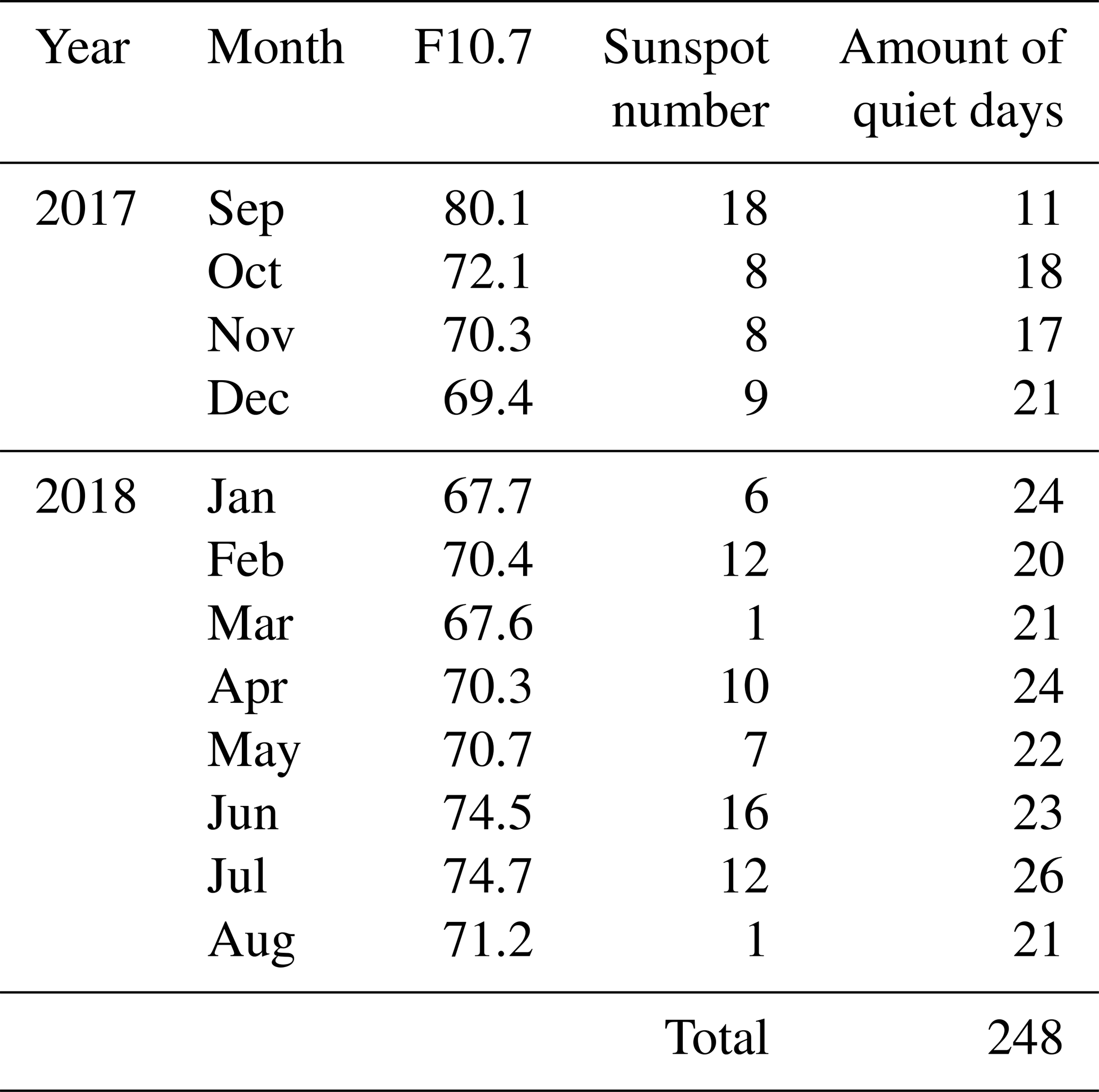
Data used in this work were collected on geomagnetically quiet days (∑ Kp ≤ 24, where ∑ Kp is the sum of the eight 3 h Kp indices for the day) from September 2017 to August 2018. The period is characterized by a very low level of solar and magnetic activity. The 27 d averaged values of the F10.7, the sunspot numbers, and the numbers of monthly quiet data used in this work are shown in Table 1. The average of the solar emission at a wavelength of 10.7 cm from September 2017 to August 2018 is only (71.6±3.5) $\times {\mathrm{10}}^{-\mathrm{22}}$ Wm⁻² Hz⁻¹, and the sunspot numbers range from 1 to 18, characterizing the period of low solar activity.

Table 1 The 27 d averaged values of F10.7, sunspot number, and the number of quiet-days from September 2017 to August 2018 considered in this work.

Monthly average values of the observed foF2, foE, and hmF2 parameters are calculated from the daily hourly values. The IRI-2016 predictions of foF2, foE, and hmF2 are computed for the same geophysical conditions to compare with the observational data and to evaluate the discrepancies and goodness of the model. The relative deviation (R_D) of the predicted values concerning the observed values for modeling the foF2 using the Consultative Committee on International Radio (CCIR) coefficient (CCIR, 1967) were computed through Eq. (1).

$$\begin{array}{}\text{(1)}& \mathit{\text{fo}}\mathrm{F}{\mathrm{2}}_{\text{CCIR-RD}}=\left({\displaystyle \frac{\mathit{\text{fo}}\mathrm{F}{\mathrm{2}}_{\mathrm{CCIR}}-\mathit{\text{fo}}\mathrm{F}{\mathrm{2}}_{\mathrm{Observed}}}{\mathit{\text{fo}}\mathrm{F}{\mathrm{2}}_{\mathrm{Observed}}}}\right)\times \mathrm{100}\mathit{\%}\end{array}$$

The term foF2_CCIR stands for the monthly average of the foF2 modeled by the CCIR sub-routine, while the term foF2_Observed is the monthly average of foF2 measured by the SMK29. Besides the comparison between the observed foF2 with CCIR, the sub-routine URSI (Rush et al., 1989) is also tested and, therefore, Eq. (1) is also used considering foF2_URSI instead of foF2_CCIR. The foF2 storm model (Araujo-Pradere et al., 2002) was turned off in the IRI-2016 options since we are interested in the quiet-time conditions. The R_D is also evaluated for hmF2 and foE using Eq. (1). For hmF2, the comparison is made using the three currently available options for determining IRI hmF2: AMTB2013 (Altadill et al., 2013), SHU-2015 (Shubin, 2015), and BSE-1979 (Bilitza et al., 1979), called AMTB, SHU, and BSE, respectively, hereafter. The AMTB model is based on ionospheric data deduced from ionograms recorded by 26 digisondes embracing latitudes from 65^∘ N to 52^∘ S and the longitude sector from 120^∘ W to 170^∘ E. The data cover different levels of solar activity from 1998 to 2006. The spherical harmonic technique was applied in AMTB to model the quiet pattern of the hmF2 at a global scale. The SHU model is based on the ionospheric radio-occultation data collected by CHAMP (from 2001 to 2008), GRACE (from 2007 to 2011), and COSMIC (from 2006 to 2012) satellite missions and ionospheric sounding data collected by 62 digisondes from 1987 to 2012. SHU uses the spherical harmonics decomposition to model hmF2. Finally, the older BSE uses the correlation between hmF2 and propagation factor M3000F2, which in turn is defined by the ratio between the highest frequency that, refracted by the ionosphere, can be detected at a distance of 3000 km (M3000) and foF2. At last, the foE comparison is made using IRI foE developed by Kouris and Muggleton (1973a, b) for CCIR (1973) with a modified zenith angle introduced by Rawer and Bilitza (1990) to improve the nighttime variations. Finally, to evaluate the performance of IRI-2016, a correlation analysis is performed between the modeled parameters and the observational data.

In some cases, the results are discussed considering the seasonal differences between the observed and modeled parameters. Each season is composed of three months as follows: December solstice (November, December, and January), March equinox (February, March, and April), June solstice (May, June, and July), and September equinox (August, September, and October). The local time (LT) in Santa Maria is defined as the universal time (UT) less three hours (LT = UT−3 h). Finally, since the focus of this work is to analyze the IRI-2016 predictions, the reader can find the complete study about the variabilities of the F2 and E layer parameters over Santa Maria during the period analyzed in the recent work by Moro et al. (2019).

3 Results

3.1 Performance of IRI in the F-region parameters

The contour plots of the monthly averaged foF2 (in MHz) observed and modeled by CCIR and URSI sub-routines, and the R_D (in percent) versus universal time (UT, vertical axis) and months (from September 2017 to August 2018, horizontal axis) are shown in Fig. 1. The foF2 values are represented by the color-coded bar on the right-hand side of panels a–c and vary from 1 to 12 MHz. The R_D in panels d–e ranges by ±50 %.

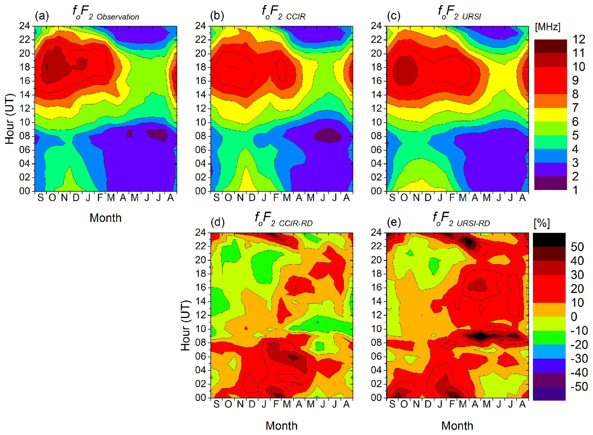
Figure 1 Contour plot of the monthly averaged foF2 (a) measured by the Santa Maria digisonde (SMK29), provided by (b) CCIR and (c) URSI coefficients. The respective relative deviation (R_D) in percent is placed in the lower panels for (d) CCIR and (e) URSI.

During the whole year analyzed the sunrise time varied from 09:15 to 10:30 UT, while the sunset took place between 20:43 and 23:30 UT over Santa Maria. The observed averaged foF2 values depicted in Fig. 1a show a diurnal variation pattern, with the highest values occurring during daytime hours (13:00–22:00 UT) and the lowest values occurring during pre-sunrise hours (around 08:00 UT). We attribute these values to the daytime dynamics over Santa Maria, e.g., photoionization and neutral atmospheric dynamics (Moro et al., 2019; Abdu and Brum, 2009). The highest values of around 11 MHz are observed between 17:00 and 20:00 UT from September to March, evidencing the seasonal trends. The lowest values of around 1.5 MHz occur between 07:00 and 09:00 UT during the June solstice months. Regarding the CCIR prediction shown in Fig. 1b and URSI predictions in Fig. 1c, foF2_CCIR and foF2_URSI, respectively, very similar diurnal and seasonal variation patterns to those seen in the observed values are observed. However, a first look at the foF2_CCIR-RD in Fig. 1d and foF2_URSI-RD in Fig. 1e reveals that the coefficient outputs grossly underestimate or overestimate the foF2 in some hours and months, as indicated below.

The foF2_CCIR-RD in Fig. 1d ranges from −20 % (underestimation) to 50 % (overestimation). The higher underestimations are observed in September and October from 09:00 to 16:00 UT, and later from November to February between 20:00 and 22:30 UT. There is also an underestimation of 20 % from April to August at around 10:00 UT. On the other hand, the overestimations are most significant during nighttime hours in almost all months from 23:00 to 08:00 UT. The foF2_URSI-RD varies from −15 % to more than 50 %. The most negative deviations are observed only in two small portions of the contour plot in Fig. 1e, which is around 21:00 UT in October, and from 18:00 to 22:00 UT in December. However, significant positive deviations higher than 50 % are seen around 09:00 UT from March to July, and in the nighttime hours around 23:00 UT from February to April. From these results, it seems that the URSI (CCIR) sub-routine overestimates (underestimates) foF2 more than the CCIR (URSI).

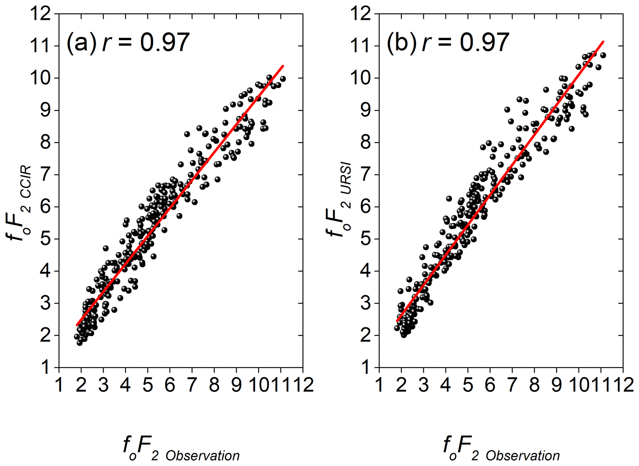
Figure 2 Scatter plots depicting the comparison between (a) foF2_CCIR and (b) foF2_URSI versus foF2_Observation.

A more detailed analysis has to be performed to further investigate the level of reliability of each IRI sub-routine. Since the data are not significantly drawn from a normally distributed population at the 0.05 % level, the quantitative estimate can be achieved by analyzing the statistical relationship between IRI foF2 and observed values using the Spearman correlation coefficient (r). The significance of the calculated r value is examined with a confidence level of 95 % between the hourly values modeled and observed data. The scatter plots of modeled IRI foF2 using CCIR and URSI coefficients versus the observational data are shown in Fig. 2. The results of the calculated r are 0.97 for both IRI coefficients. An almost perfect positive correlation is shown.

The contour plots of the monthly averaged hmF2 (in km) observed by the SMK29 and modeled by AMTB, SHU, and BSE sub-routines and the R_D (in percent) versus universal time (UT, vertical axis) and month (from September 2017 to August 2018, horizontal axis) are shown in Fig. 3. The color-coded bar on the right-hand side of panels a–d represent hmF2 ranging from 180 to 360 km. In panels e–g, the color-coded bar refers to the R_D and ranges ±50 % for the three plots. The observed hmF2 values in Fig. 3a show that the F2-layer is higher during nighttime hours, achieving 340 km from September to December from 01:00 UT to around 03:00 UT. There is also more intense hmF2 values between 300 and 320 km during the September equinox and December solstice months from 12:00 to 18:00 UT. The daytime average values in the March equinox and June solstice months are usually below 240 km. The more intense values during nighttime in all months and in the daytime during the September equinox and December solstice months are quite well represented by the AMTB in Fig. 3b, SHU in Fig. 3c, and BSE in Fig. 3d as well as the low values during the daytime from the March equinox and June solstice months. Although there are similarities, IRI-2016 predictions have some different aspects, as shown by the hmF2_AMTB-RD in Fig. 3e, hmF2_SHU-RD in Fig. 3f, and hmF2_BSE-RD in Fig. 3g. A visual comparative analysis shows that the SHU agrees better with the observations since the RD encompasses, in general, ±10 % most of the time. The same is not true for AMTB and BSE predictions.

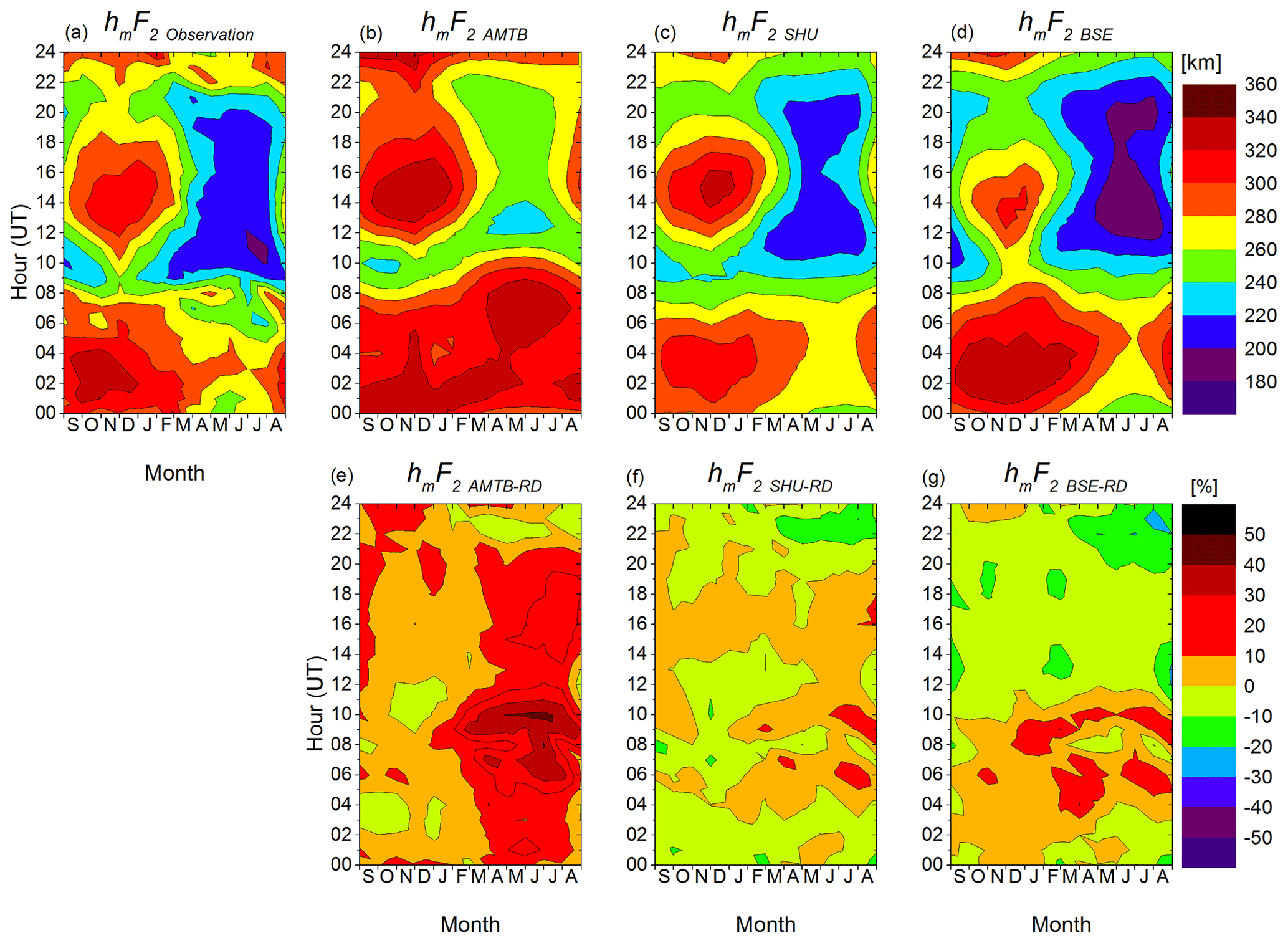
Figure 3 Contour plot of the monthly averaged hmF2 (a) measured by the Santa Maria digisonde (SMK29), provided by (b) AMTB, (c) SHU, and (d) BSE coefficients. The respective relative deviation (R_D) in percent is placed in the lower panels for (e) AMTB, (f) SHU, and (g) BSE.

The hmF2_AMTB-RD ranges from −10 % to 43 %. The main differences are related to the overestimation of hmF2 most of the time in September and October and from March to August as represented by the hottest color of the palette. It differs in particular near the sunrise period from 07:00 to 11:00 UT in the June equinox. The hmF2_SHU-RD varies from −20 % to 20 %. In general, the SHU outputs differ only ±10 % from the observation results, revealing very good agreement with the observations. Regarding hmF2_BSE-RD, it ranges from −24 % to 20 %. There are some small periods near sunrise (sunset) in which hmF2 is overestimated (underestimated), but in general, BSE also represents the observations well. As shown by the results presented in Fig. 3, SHU and BSE perform better than AMTB in modeling hmF2. This result is also confirmed by the statistical relationship shown by the Spearman r values shown in Fig. 4. Modeling the hmF2 with the SHU coefficients presents the best scenario with the r=0.86, as shown in Fig. 4b. Despite the AMTB in Fig. 4a presenting the lower correlation (r=0.72), it is important to note that it is still significant.

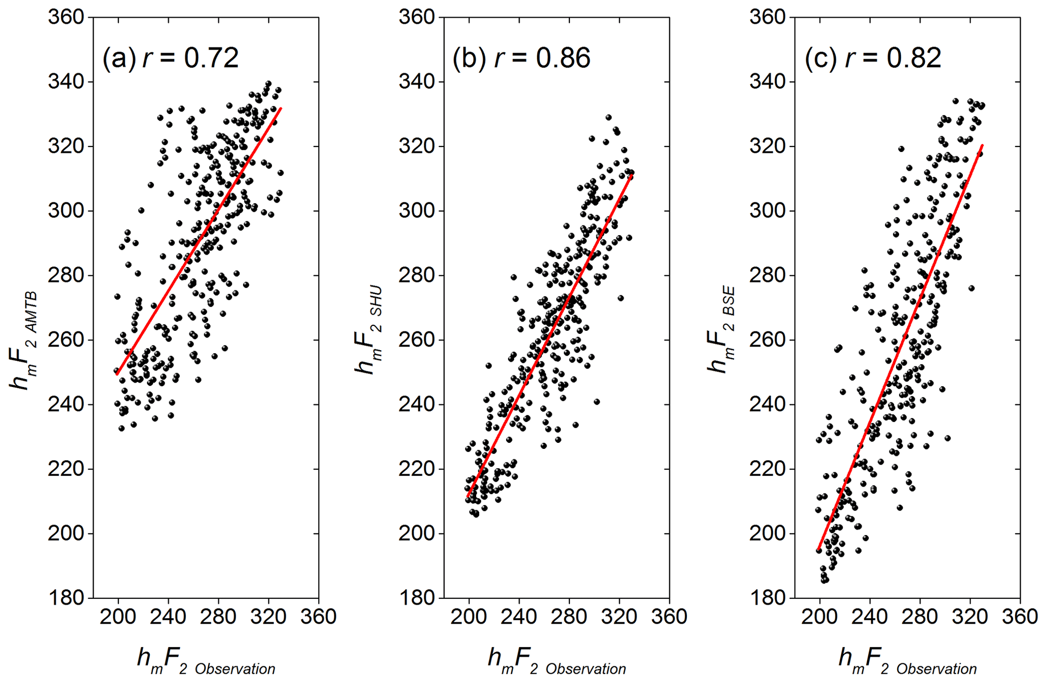
Figure 4 Scatter plots depicting the comparison between (a)  hmF2_AMTB, (b)  hmF2_SHU, and (c)  hmF2_BSE versus hmF2_Observation.

3.2 Performance of IRI foE

The contour plots of the monthly averaged foE (in MHz) observed by the SMK29 and modeled by IRI-2016 and the estimated R_D (in percent) versus universal time (UT, vertical axis) and month (from September 2017 to August 2018, horizontal axis) are shown in Fig. 5. The foE values are represented by the color-coded bar on the right-hand side, ranging from 1 to 3.5 MHz for the critical frequency in panels a–b, and ±20 % for the R_D in panel c.

Figure 5 Contour plot of the monthly averaged foE (a) measured by the Santa Maria digisonde (SMK29), provided by (b) IRI, and (c) the relative deviation (R_D) in percent.

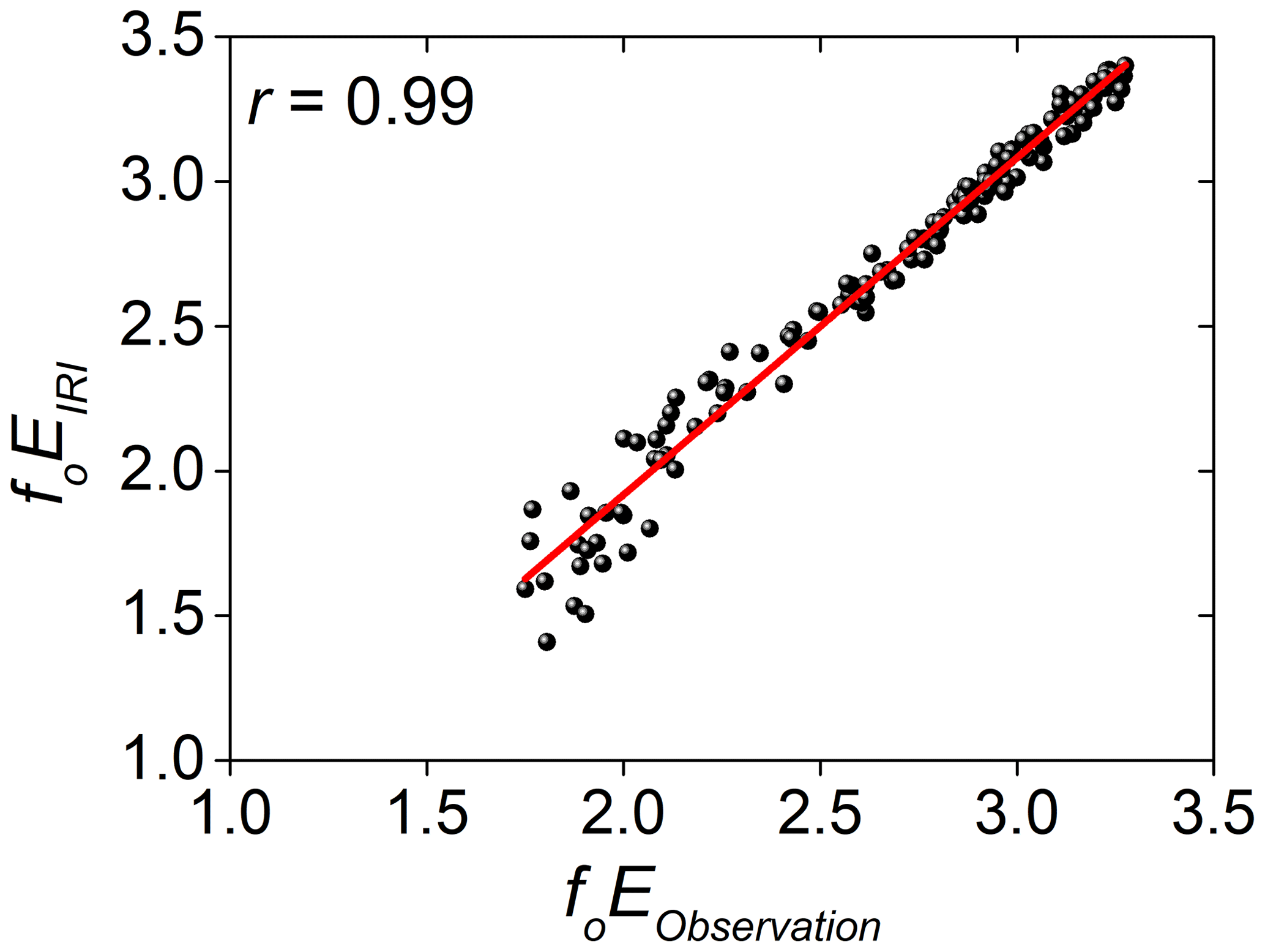
The observed foE in Fig. 5a shows a regular diurnal variation, increasing from sunrise to a peak in the afternoon to around 3.5 MHz, and falling until sunset. The low electron density at night makes it difficult to detect the E region by the digisonde. The most intense values of around 3.5 MHz are seen during the September equinox and December solstice months. The agreement between IRI foE and observations is very good, as shown in Fig. 5b. The maxima values seen in IRI occur for longer than in the observations, however. They are shifted two months (April and May) and start earlier (July). The foE_IRI-RD in Fig. 5c are positive (overestimation) up to 5 % only, confirming the good IRI-2016 performance in modeling foE almost all the time over Santa Maria. There are some considerable differences in a short time in the sunrise and sunset hours. These are critical periods which may be caused by distortions in the E-region traces due to horizontal gradients in the ionosphere, making it difficult to model with IRI, as can be expected by the users. The r value obtained between the modeled and observed values is the highest in this work, showing a very strong positive correlation, as shown in Fig. 6.

Figure 6 Scatter plot depicting the comparison between foE_IRI versus foE_Observation.

4 Discussion

The focus of this work is to use the foF2, foE, and hmF2 measured by the recent digisonde installed in Santa Maria, Brazil, to test the performance of the IRI-2016 in the low-latitude ionosphere situated close to the center of the SAMA during the geomagnetically quiet days from September 2017 to August 2018. The results presented in Figs. 1 and 2 show that the foF2 predictions obtained with CCIR and URSI coefficients are very similar in a month-by-month analysis. However, CCIR (URSI) underestimates (overestimates) foF2 during specific nighttime hours. When the whole period of data is considered, both coefficients gave r equal to 0.97. The correlation is an indication that the model accurately predicts the diurnal and seasonal trends of foF2 over Santa Maria. In general, the IRI user may choose any sub-routine to model foF2.

The results obtained in this work closely follow the earlier work of Ezquer et al. (2008), who had compared the CCIR and URSI coefficients with the ionosonde data in Tucumán. They report that, in general, both coefficients give comparable values. However, they also report disagreements among predictions and measurements reaching values of R_D close to 50 %. In the Brazilian sector, Batista and Abdu (2004) in a similar comparative study pointed out that the agreements between the URSI values and the observed foF2 in São Luís were always better as compared to the CCIR coefficients. They also showed that the foF2 after sunset is overestimated for the equatorial station of São Luís. It seems that over the Brazilian territory the right choice between CCIR and URSI in modeling foF2 depends on the location of the users. In the Brazilian equatorial region, CCIR performs better, while in the SAMA region there are no appreciable differences between both. In China, Liu et al. (2019) found that the CCIR performs better than URSI during post-sunset under low solar activity or in the EIA region. For other times and outside the EIA region over China CCIR shows no large difference in performance as compared to URSI.

Figures 3 and 4 show that the SHU option for modeling the hmF2 performs better over Santa Maria, followed by BSE, and the AMTB is the worst. The r value of AMTB is 0.72, the lowest observed in the present study. It is even lower than the older BSE coefficient used in the previous versions of the IRI model. Overall, the AMTB (BSE) overestimated (underestimated) the observed values. Therefore, it is recommended to use the SHU option when modeling the hmF2 over Santa Maria. These results agree with the findings of Zhao et al. (2017), who also recommend the use of SHU option over China region when using IRI-2016 to model hmF2. Since this is the first evaluation of the three IRI hmF2 options in the Brazilian sector to the author's knowledge, there is no comparison between our work with other Brazilian equatorial or low latitude regions, and this is suggested for a future study.

Finally, the comparative results presented in Figs. 5 and 6 show that the IRI-predicted foE values are in excellent agreement with observations in Santa Maria. The calculated r value is 0.99. The strong correlation may be explained by the fact that the E region ionization is subject to solar radiation control, and therefore IRI predicts the E region solar ionization fairly accurately everywhere across the globe since there is no plasma transport in the E region.

5 Conclusions

The present work uses the foF2, foE, and hmF2 parameters acquired by a recent digisonde installed in Santa Maria, Brazil, close to the center of the SAMA, to test the performance of the IRI-2016. Only data collected under geomagnetically quiet conditions from September 2017 to August 2018 are used to eliminate the effects of geomagnetic disturbances. Monthly average values of the observed ionospheric parameters are calculated from the daily hourly values and compared with the IRI-2016 predictions for the same geophysical conditions. The relative deviation (R_D) was computed using the CCIR and URSI coefficients to estimate the IRI foF2 performance. The IRI hmF2 predictions are evaluated using the R_D estimated using the three options AMTB, SHU, and BSE. The IRI foE performance is also tested. The main findings of the study are as follows:

• a.

  CCIR and URSI predictions represent the diurnal and seasonal variation patterns of the observed values. foF2_CCIR-RD ranges from −20 % (underestimation) to 50 % (overestimation). The higher underestimations are observed in September and October from 09:00 to 16:00 UT, and later from November to February between 20:00 and 22:30 UT. There is also an underestimation of 20 % from April to August at around 10:00 UT. The overestimations are most significant during nighttime hours during almost all months from 23:00 to 08:00 UT. The foF2_URSI-RD varies from −15 % to more than 50 %. The most negative deviations are observed at around 21:00 UT in October, and from 18:00 to 22:00 UT in December. Significant positive deviations higher than 50 % are seen at around 09:00 UT from March to July, and in the nighttime hours around 23:00 UT from February to April.

• b.

  SHU agrees better with the observations than AMTB and BSE for modeling hmF2. The hmF2_AMTB-RD ranges from −10 % to 43 %. The main differences are related to the overestimation of hmF2 most of the time in September and October and from March to August. It differs in particular near the sunrise period from 07:00 to 11:00 UT in June equinox. The hmF2_SHU-RD varies from −20 % to 20 % and, in general, differs by only ±10 % from the observation. The results reveal very good agreement with the observations. hmF2_BSE-RD ranges from −24 % to 20 %. There are some small periods near sunrise (sunset) in which hmF2 is overestimated (underestimated), but in general, BSE also represents the observations well.

• c.

  The agreement between IRI foE and observations is very high. However, the maxima values seen in IRI occur for longer than in the observations, as well as being shifted two months (April and May) and starting earlier (July). The foE_IRI-RD values are positive (overestimation) up to 5 % only, confirming the good IRI-2016 performance in modeling foE almost all the time over Santa Maria, except for a short time in the sunrise and sunset hours.

As a general conclusion of this work, it is shown that both CCIR and URSI coefficients have high accuracy in predicting foF2 over Santa Maria. The same is true for IRI foE. However, it is recommended that the users use the SHU coefficient as the first option to model hmF2 over Santa Maria, which is different from the recommendation of IRI-2016.