A deep insight into the ion foreshock with the help of test particle two-dimensional simulations

Two-dimensional (2D) test particle simulations based on shock profiles issued from 2D full particle-in-cell (PIC) simulations are used in order to analyze the formation processes of ions back streaming within the upstream region after interacting with a quasi-perpendicular curved shock front. Two different types of simulations have been performed based on (i) a fully consistent expansion (FCE) model, which includes all self-consistent shock profiles at different times, and (ii) a homothetic expansion (HE) model in which shock profiles are fixed at certain times and artificially expanded in space. The comparison of both configurations allows one to analyze the impact of the front nonstationarity on the back-streaming population. Moreover, the role of the space charge electric field E_l is analyzed by either including or canceling the E_l component in the simulations. A detailed comparison of these last two different configurations allows one to show that this E_l component plays a key role in the ion reflection process within the whole quasi-perpendicular propagation range. Simulations provide evidence that the different field-aligned beam (FAB) and gyro-phase bunched (GPB) populations observed in situ are essentially formed by a E_t×B drift in the velocity space involving the convective electric field E_t. Simultaneously, the study emphasizes (i) the essential action of the magnetic field component on the GPB population (i.e., mirror reflection) and (ii) the leading role of the convective field E_t in the FAB energy gain. In addition, the electrostatic field component E_l is essential for reflecting ions at high θ_Bn angles and, in particular, at the edge of the ion foreshock around 70^∘. Moreover, the HE model shows that the rate BI_% of back-streaming ions is strongly dependent on the shock front profile, which varies because of the shock front nonstationarity. In particular, reflected ions appear to escape periodically from the shock front as bursts with an occurrence time period associated to the self-reformation of the shock front.

1 Introduction

While upstream ions of the incoming solar wind interact with the curved terrestrial bow shock, a certain percentage is reinjected back into the solar wind and propagates along the interplanetary magnetic field (IMF); they form the so-called ion foreshock. This population has been extensively studied both with the help of experimental data (Tsurutani and Rodriguez, 1981; Paschmann et al., 1981; Bonifazi and Moreno, 1981a, b; Fuselier, 1995; Eastwood et al., 2005; Oka et al., 2005; Kucharek, 2008; Hartinger et al., 2013) and numerical simulations (Blanco-Cano et al., 2009; Lembège et al., 2004; Savoini et al., 2013; Kempf et al., 2015; Savoini and Lembège, 2015; Otsuka et al., 2018).

Even if we restrict ourselves to the quasi-perpendicular region (i.e., for $\mathrm{45}{}^{\circ }\le {\mathit{\theta }}_{\mathrm{Bn}}\le \mathrm{90}{}^{\circ }$, where θ_Bn is the angle between the local shock normal and the IMF), different types of back-streaming ions are identified, and (a) some are characterized by a gyrotropic velocity distribution and form the field-aligned ion beam population (hereafter FAB); conversely, (b) others exhibit a nongyrotropic velocity distribution and form the gyro-phase bunched ion population (hereafter GPB). None of these populations yet have a well-established origin, and different mechanisms have been proposed for years (Möbius et al., 2001; Kucharek et al., 2004), including (i) scenarios based on the specular reflection (Sonnerup, 1969; Paschmann et al., 1980; Schwartz et al., 1983; Schwartz and Burgess, 1984; Gosling et al., 1982) with or without the conservation of the magnetic moment and (ii) scenarios which invoke the leakage of some magnetosheath ions producing a low-energy FAB population (Edmiston et al., 1982; Tanaka et al., 1983; Thomsen et al., 1983). Nevertheless, the origin of FAB ions could be due to (iii) the diffusion of some reflected ions (called gyrating ions; these ions are reflected by the supercritical shock front but do not manage to escape into the upstream region and go into the downstream region after their initial gyration (Schwartz et al., 1983)). The diffusion can either be generated by upstream magnetic fluctuations (Giacalone et al., 1994) or more directly by the shock ramp itself (with a pitch angle scattering during the reflection process) (Kucharek et al., 2004; Bale et al., 2005). All scenarios have some drawbacks and are not able to clearly explain the origin of both populations. On the other hand, GPB are preferentially observed at some distance from the curved shock front (Thomsen et al., 1985; Fuselier et al., 1986a), and their synchronized nongyrotropic distribution is part of a low-frequency monochromatic waves trapping (Mazelle et al., 2003; Hamza et al., 2006), or of beam plasma instabilities (Hoshino and Terasawa, 1985). As a conclusion, it is quite difficult to discriminate between these different scenarios which can be present simultaneously or separately in time.

Our previous papers (Savoini et al., 2013; Savoini and Lembège, 2015) were focused on the origin of these two populations. A large-scale, two-dimensional particle-in-cell (PIC) simulation of a curved shock has been used, where full curvature and time-of-flight effects for both electrons and ions are self-consistently included. Our simulations have shown that both FAB and GPB populations and their typical associated pitch angle distributions observed experimentally (Fuselier et al., 1986b; Meziane, 2005) have been retrieved not far from the front (up to 2–3R_E, where R_E is the Earth's radius). Moreover, results have shown that these two populations can be generated directly by the macroscopic electric E and magnetic B fields present at the shock front itself. In other words, the differences observed between FAB and GPB populations are not the result of distinct reflection processes but are the consequence of the time history of ions interacting with the shock front. The FAB population loses their initial phase coherency by suffering several bounces along the front, which is in contrast with the GPB population which suffers mainly one bounce (i.e., mirror reflection process). This important result was not expected and greatly simplifies the question on each population origin (Savoini and Lembège, 2015)

Nevertheless, some further questions, which are difficult to investigate with full PIC simulations (because of the self-consistency), still need to be answered in order to analyze several aspects of the reflection process. For this reason, we use complementary test particle simulations herein to clarify the respective impact of the shock curvature and the time variation in the macroscopic fields at the shock front on the back-streaming ion reflection process. The main questions presently addressed are summarized as follows:

1. Is the reflection process noncontinuous in time (burst-type reflection process) or not? In this case, how is it linked to the θ_Bn angle variation (i.e., space dependence) and/or to the shock profile variation (i.e., time dependence)?

2. What is the impact of the space charge electric field localized within the shock ramp on the reflection process?

3. What kind of reflection mechanisms can be identified in present simulations?

The paper is organized as follows. Section 2 briefly summarizes the conditions of the previous 2D PIC simulations (Savoini and Lembège, 2015) and of present particle test simulations. In Sects. 3 and 4, results of test particles are presented, and the ion reflection processes are investigated. The discussion and conclusions will be presented in Sects. 5 and 6, respectively.

2 Numerical simulation conditions

The numerical conditions concerned in the present paper are similar to those described in Savoini et al. (2013) and Savoini and Lembège (2015). In short, we used a 2D, fully electromagnetic, relativistic particle code based on a standard finite-sized particle technique (similar to Lembège and Savoini, 1992, 2002 for planar shocks).

2.1 Self-consistent full PIC simulations

The code solves Maxwell and Poisson's equations in the Fourier space (so-called pseudospectral code), which allows one to separate the electric field contribution in two distinct parts, namely (i) a longitudinal or electrostatic component, hereafter denoted by subscript _l (built up by the space charge effects $\mathbf{\nabla }{\mathit{E}}_{\mathrm{l}}=\mathit{\rho }/{\mathit{ϵ}}_o$), and (ii) a transverse or induced component, hereafter denoted by subscript _t (coming from the temporal variations in the magnetic field $\mathbf{\nabla }\times {\mathit{E}}_{\mathrm{t}}=-\partial \mathit{B}/\partial t$). The longitudinal component is essentially built up within the shock front due to the different dynamics of ions and electrons, whereas the induced component is mainly generated by the propagating shock front itself (see Fig. 1, panel 2a) through the convective term ${\mathit{E}}_{\mathrm{t}}=-\mathit{U}\times \mathit{B}$ (where U corresponds to the bulk shock front velocity since we are in the solar wind frame). In addition, the subscripts _∥ and _⟂ stand for parallel and perpendicular directions to the local magnetic field, respectively. In Fig. 1 and in following, the X–Y reference frame is the solar wind frame, with the third direction along Z pointing backward into the plot. Then, E_t has the direction of the increasing Y, and ∇B has the same direction as the present U vector.

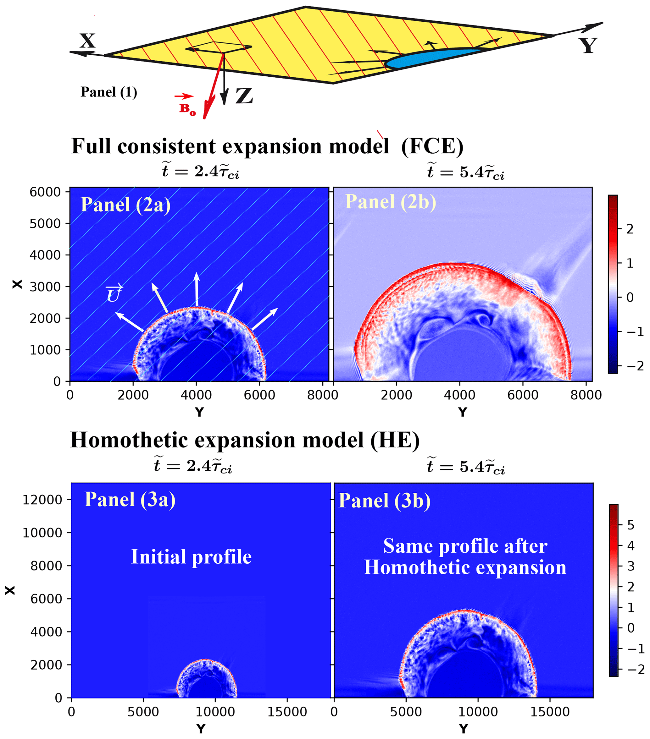
Figure 1 Panel (1) plots the simulation plane geometry; the ${\stackrel{\mathrm{̃}}{B}}_o$ magnetostatic field is mainly outside and directed downward from the plane. Panels (2a, b) illustrate the evolution of the magnetic field ${\stackrel{\mathrm{̃}}{B}}_{\mathrm{tz}}$ in the fully consistent expansion (FCE) model (time dependent), respectively, at ${\stackrel{\mathrm{̃}}{t}}_{\mathrm{init}}=\mathrm{2.4}{\stackrel{\mathrm{̃}}{\mathit{\tau }}}_{\mathrm{ci}}$ and ${\stackrel{\mathrm{̃}}{t}}_{\mathrm{simul}}=\mathrm{5.4}{\stackrel{\mathrm{̃}}{\mathit{\tau }}}_{\mathrm{ci}}$. In panel (2a), used as a reference, the vector velocity $\stackrel{\mathrm{̃}}{U}={\stackrel{\mathrm{̃}}{v}}_{\mathrm{shock}}$ has been superimposed to illustrate the shock front propagation (white thick arrows); the arrow length is not at the right scale. In addition, the projection of the ${\stackrel{\mathrm{̃}}{B}}_o$ magnetic field lines has been reported (oblique white thin lines). Panels (3a, b) illustrate one example of the curved magnetic field ${\stackrel{\mathrm{̃}}{B}}_{\mathrm{tz}}$ in the homothetic expansion (HE) model (time independent), where the shock profile is fixed in time but expands in space via an expanding factor proportional to the shock front velocity v_shock×t; this shock profile has been chosen at the time ${\stackrel{\mathrm{̃}}{t}}_{\mathrm{init}}=\mathrm{2.4}{\stackrel{\mathrm{̃}}{\mathit{\tau }}}_{\mathrm{ci}}$ of the self-consistent simulation. From this time, the shock front dilates by a factor of 2.6 compared to its initial shape.

In our configuration, the magnetostatic field is partially lying outside the simulation plane (see Savoini and Lembège, 2001 for more details). Then, the simulation is limited to the whole quasi-perpendicular shock (i.e., for $\mathrm{45}{}^{\circ }\le {\mathit{\theta }}_{\mathrm{Bn}}\le \mathrm{90}{}^{\circ }$). We use a magnetic piston for which the geometry is adapted to initiate a shock front with a curvature radius large enough to be compared with the upstream ion Larmor gyroradius ${\stackrel{\mathrm{̃}}{\mathit{\rho }}}_{\mathrm{ci}}$ (all normalized quantities are indicated with a tilde $\stackrel{\mathrm{̃}}{}$); this is the same normalization which is used in the previous self-consistent PIC simulations (Savoini and Lembège, 2001; Savoini et al., 2013; Savoini and Lembège, 2015). The curvature increases during the simulation. This configuration has two consequences; (i) first, as the time increases and the shock front expands, its velocity slightly decreases and so does the Alfvén Mach Number M_A from ≈5 to ≈3, where the velocity is measured at ${\mathit{\theta }}_{\mathrm{Bn}}=\mathrm{90}{}^{\circ }$ used as a reference angle; (ii) the time-of-flight effects are self-consistently included. Indeed, this ballistic process is observed when the upstream magnetic field lines are convected by the incoming solar wind. In present simulations (based on upstream rest frame), the curved shock front expands and scans different θ_Bn values. As a result, back-streaming particles, collected at a given upstream location, come from different parts of the curved shock front, depending on their respective velocity.

Initial plasma conditions are summarized as follows: light velocity $\stackrel{\mathrm{̃}}{c}=\mathrm{3}$ and temperature ratio between ion and electron population $T_{\mathrm{el}}/T_{\mathrm{io}}=\mathrm{1.58}$. A mass ratio $m_i/m_e=\mathrm{84}$ is used in order to save CPU time, and the Alfvén velocity is ${\stackrel{\mathrm{̃}}{v}}_{\mathrm{A}}=\mathrm{0.16}$. The number of cells in the simulation plane along each axis is NCX = NCY $=\mathrm{8192}\approx \mathrm{150}{\stackrel{\mathrm{̃}}{\mathit{\rho }}}_{\mathrm{ci}}$, with the size of a grid cell ${\mathrm{\Delta }}_x=\mathrm{\Delta }y\approx \mathrm{1}{\stackrel{\mathrm{̃}}{\mathit{\rho }}}_{ce}$. The shock is in the supercritical regime. with a time-averaged Alfvén Mach number M_A≈4 measured at ${\mathit{\theta }}_{\mathrm{Bn}}=\mathrm{90}{}^{\circ }$. In order to observe the early stage of the ion foreshock formation, the end time of the simulation is ${\stackrel{\mathrm{̃}}{t}}_{\mathrm{simul}}=\mathrm{5.4}{\stackrel{\mathrm{̃}}{\mathit{\tau }}}_{\mathrm{ci}}$ (where ${\stackrel{\mathrm{̃}}{\mathit{\tau }}}_{\mathrm{ci}}$ is the upstream ion gyro-period), which is large enough to investigate the interaction of incoming ions with the shock front and the further formation of back-streaming ions.

2.2 Test particle simulations

In the present paper, we use all field components issued from the same previous PIC simulation as in Savoini and Lembège (2015); all components have been saved every $\mathrm{\Delta }\stackrel{\mathrm{̃}}{T}={\stackrel{\mathrm{̃}}{\mathit{\tau }}}_{\mathrm{ci}}/\mathrm{20}$. Test particle simulations appear to be a straightforward way to evaluate the action of different field components on the ion dynamics. Indeed, the feedback effects of particles on electromagnetic fields are excluded in test particle simulations, and one can modify or cancel some field components independently from each other. This allows one to identify their specific actions on particles and on the resulting ion reflection processes.

Figure 1 plots an example of the two configurations used hereafter in this paper. Panels 2a–b show the fully consistent expansion model (hereafter named FCE), which corresponds to the results where test ions interact with the E and B fields issued from the self-consistent simulation and where both spatial inhomogeneities and nonstationarities are fully included. If this configuration is easy to understand, the so-called particular approach named the homothetic expansion model (hereafter named HE) shown in panels 3a–b is complementary. In this case, particles interact with a propagating fixed front profile, i.e., all-time profile variations are excluded; only spatial inhomogeneities of the shock front profile chosen at the selected time are included, as detailed in Sect. 4.

In the two configurations of FCE and HE, we inject test particles distributed within 10 individual sampling boxes located along the curved shock front (Fig. 2). This procedure allows us to analyze the impact of the front curvature (local θ_Bn) on the formation of back-streaming ions. We follow a total of 1 million test particles. Then, each box has the same number of particles N=100 000, and they are initialized as a Maxwellian distribution with a thermal velocity v_thi, which is the same as in the self-consistent simulation (Savoini and Lembège, 2015).

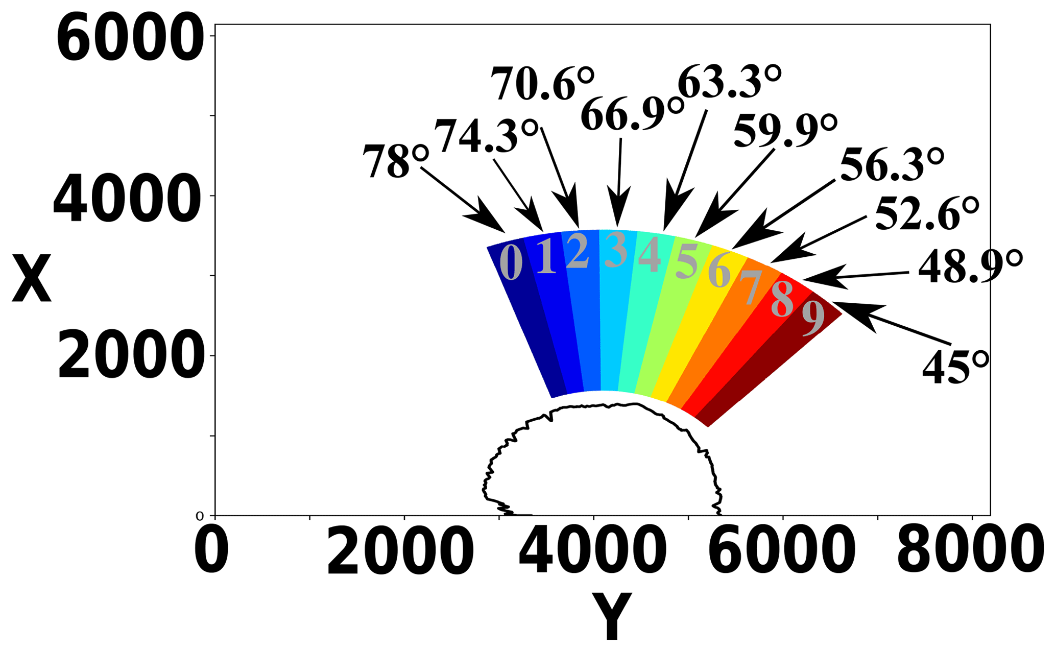
Figure 2 Initial location of the 10 sampling boxes (labeled from zero to nine) which map the upstream ion foreshock region. All ions belonging to a given box are represented by the same color for statistical analysis only (Sects. 3 and 4). The θ_Bn propagation angle, where each box is initially centered at time t=0, is reported above the corresponding identification number of the box, but these colors will not be used anymore in this paper.

Let us point out that the use of finite-sized sampling boxes at different initial θ_Bn angles only estimates the location where the particles hit the shock but does not provide an exact value for the local θ_Bn seen by the particles when these interact with the expanding shock front. Nevertheless, it is quite helpful when classifying the different types of particle interactions with the curved front. The sizes of all the identical boxes are chosen so that (i) along the curved shock front each box has an angular extension of $\approx \mathrm{4}{}^{\circ }$, which is small enough to scan the different orientations of θ_Bn and large enough for statistical constraints, and (ii) along the local shock normal, where each box has a length large enough (L_size=2000Δx) to ensure that most particles interact with the shock front during a noticeable time range (i.e., $D_T\approx \mathrm{3}{\stackrel{\mathrm{̃}}{\mathit{\tau }}}_{\mathrm{ci}}$).

Then, Sect. 3 will present the results obtained in the FCE model, which is the usual configuration representing the time evolution of test particles with the self-consistent shock front profile. Section 4 will then introduce the more unusual HE expansion model (i.e., homothetic simulation approach).

3 Numerical results: the fully consistent expansion model (FCE)

To clarify the presentation, we will split this section into two parts in which we analyze, respectively, (i) the dynamics of the back-streaming ions (alias BI) in the different boxes and their main features, in terms of spatial and time evolution, and (ii) their behavior when some field components at the shock front are included/artificially excluded.

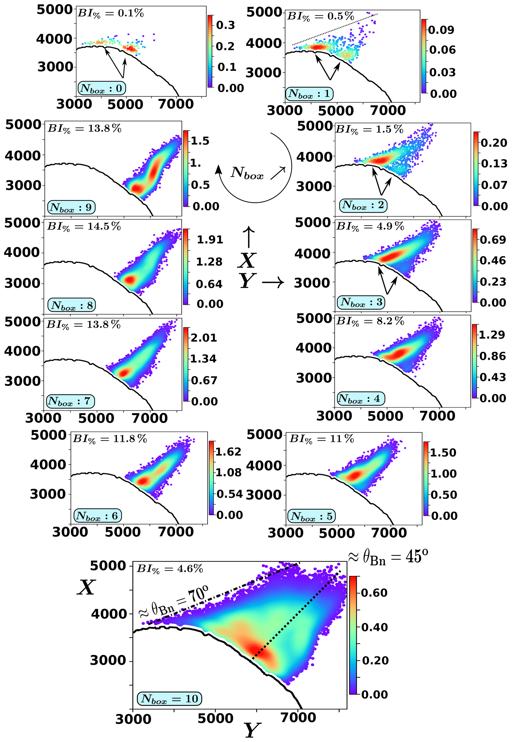
Figure 3 FCE configuration: spatial distribution of the back-streaming particle density within the simulation X–Y plane at the end of the simulation time (${\stackrel{\mathrm{̃}}{t}}_{\mathrm{end}}\approx \mathrm{5.4}{\stackrel{\mathrm{̃}}{\mathit{\tau }}}_{\mathrm{ci}}$, where ${\stackrel{\mathrm{̃}}{\mathit{\tau }}}_{\mathrm{ci}}$ is the upstream ion cyclotron period). All boxes are plotted from N_Box=0 to 9, defined initially at ${\mathit{\theta }}_{\mathrm{Bn}}\approx \mathrm{90}{}^{\circ }$ and $\approx \mathrm{45}{}^{\circ }$, respectively; the bottom panel labeled N_Box=10 shows aggregate boxes in which we have reported the edge of the ion foreshock (dashed line) and the angle ${\mathit{\theta }}_{\mathrm{Bn}}=\mathrm{45}{}^{\circ }$ (dotted line) for reference. Considering the small number of ions involved in the reflection process, we have used a Gaussian interpolation which gives the relative density weight of each ion. Then, the color coding (vertical bar) gives only an indication of the relative density amplitude. The location of the curved shock front is defined at the middle of the front ramp (thick black line) at the last time ${\stackrel{\mathrm{̃}}{t}}_{\mathrm{end}}$. Moreover, we have reported the space-integrated percentage value BI_% of back-streaming ions within each corresponding box. In order to exclude the gyrating ions present near the front from the back-streaming population, we have eliminated ions found within a small area ≈2–3ρ_ci upstream of the shock front. For this reason, a very thin white area is visible along the curved front where no particles are present. For N_Box=0–3, the arrows point to the two spots (see the text for explanations). The edge of the foreshock is represented by a mixed line at θ_Bn=70^∘. The dashed line (defined for θ_Bn=45^∘) is indicated for reference.

3.1 General features of the back-streaming ions

Figure 3 plots the spatial distribution of the back-streaming ions' density for the different sampling boxes (defined in Fig. 2) at the end time of the simulation for the FCE model. Different information can be summarized as follows:

• i.

  The percentage of the back-streaming ions BI_% is obtained by computing the ratio of the back-streaming ions over the number of ions which have interacted with the shock front. This number increases when moving further into the foreshock (i.e., for decreasing θ_Bn) from BI_%=0.1 for N_Box=0 to BI_%≈14 for N_Box=9. This θ_Bn dependence is in agreement with previous experimental observations (Ipavich et al., 1981; Eastwood et al., 2005; Mazelle et al., 2005; Turner et al., 2014) and numerical simulations (Savoini and Lembège, 2015; Kempf et al., 2015).

• ii.

  The upstream edge of the ion foreshock (mixed line in Fig. 3 for N_Box=10) is not parallel to the IMF but is the result of the time-of-flight effect included in our simulations (Savoini et al., 2013). At the end of the simulation, this edge starts from the shock at the same critical angle, the so-called ${\mathit{\theta }}_{\mathrm{io},\mathrm{fore}}\approx \mathrm{70}{}^{\circ }$, as found in our previous self-consistent simulations (Savoini et al., 2013; Savoini and Lembège, 2015).

• iii.

  The back-streaming ion density is not uniform along the shock normal but exhibits different maxima, according to our observations. Not only is the spatial distribution not the same for all boxes but is even not uniform within a given same box, i.e., back-streaming ions do not escape uniformly away from or along the shock front. For instance, boxes N_Box=0–3 evidence two distinct spots near the shock front, as indicated by black arrows. As θ_Bn decreases (i.e., N_Box=5–9), the right-hand spot disappears and the back-streaming population increasingly aligns along the upstream magnetic field B_o. Accordingly, the width of the reflection area (i.e., the angular extension of the ion foreshock defined very near the shock front) shrinks from ≈50ρ_ci (for N_Box=0) to ≈17ρ_ci (for N_Box=9).

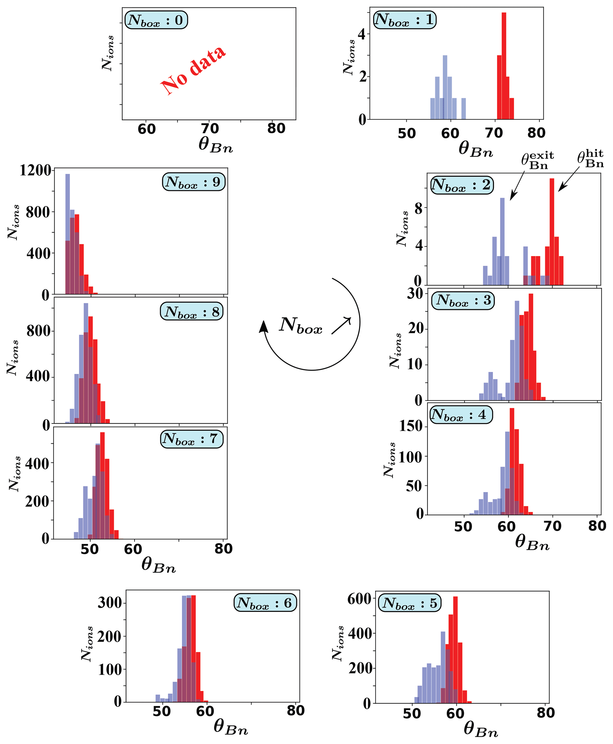
These two distinct spots may be explained by the different time histories of the back-streaming ions within the shock front, as reported in Savoini and Lembège (2015). Actually, the interaction time strongly differs from one ion to another, depending on its gyrating feature when it hits the shock front for the first time. Short and long interactions over time can be defined, depending on whether the reflection process is respectively associated to a short or long displacement of the ion along the shock front before escaping upstream. If the individual trajectory of the reflected ions has been already evidenced in Savoini and Lembège (2015), present test particle simulations allow one to generalize the results via a statistical approach versus their initial angular locations (i.e., the N_Box number). Figure 4 plots the distribution of θ_Bn angles seen by the particles when these hit for the first time the shock front (hereafter named ${\mathit{\theta }}_{\mathrm{Bn}}^{\mathrm{hit}}$ in red) and when they finally exit the shock front to escape upstream (hereafter named ${\mathit{\theta }}_{\mathrm{Bn}}^{\mathrm{exit}}$ in blue). These statistical results are obtained by computing these angles for each particle. As a consequence, angle values are computed neither at the same time nor at the same location along the curved front (even if they are initially located in the same box). In other words, each particle sees different local shock front profiles in terms of the spatial inhomogeneity and time nonstationarity of the shock front.

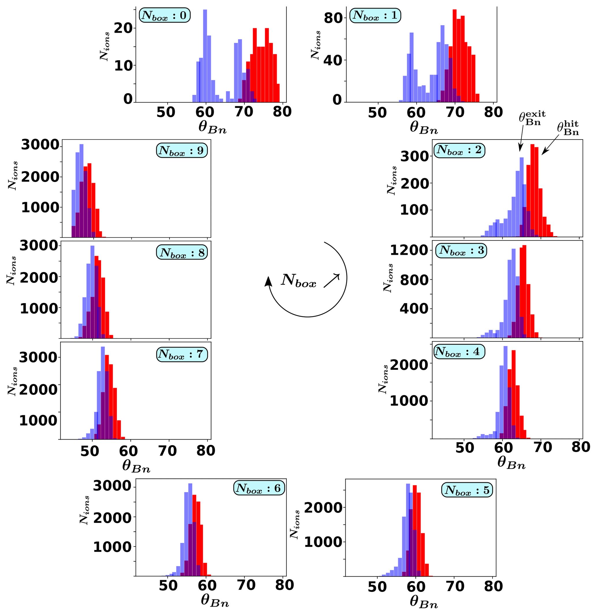
Figure 4 FCE configuration: plots of the ion distribution functions for each box N_Box=0–9 versus the local θ_Bn angle computed when ions hit the shock front for the first time (red distribution function of the so-called ${\mathit{\theta }}_{\mathrm{Bn}}^{\mathrm{hit}}$) and when these leave and escape upstream (blue distribution function versus the so-called ${\mathit{\theta }}_{\mathrm{Bn}}^{\mathrm{exit}}$). The angles ${\mathit{\theta }}_{\mathrm{Bn}}^{\mathrm{hit}}$ and ${\mathit{\theta }}_{\mathrm{Bn}}^{\mathrm{exit}}$ have been reported in N_Box=2 for reference.

First, let us note that the averaged value of ${\mathit{\theta }}_{\mathrm{Bn}}^{\mathrm{hit}}$ corresponds mainly to the initial location of the box, and therefore, the most important feature is not the angle values themselves but rather the difference between the averaged values of ${\mathit{\theta }}_{\mathrm{Bn}}^{\mathrm{hit}}$ and ${\mathit{\theta }}_{\mathrm{Bn}}^{\mathrm{exit}}$ when ions hit and leave the shock front, respectively. For this reason, we will use the angular range of the particles' interaction with the front as defined by ${\mathrm{\Delta }}_{\mathrm{int}}{\mathit{\theta }}_{\mathrm{Bn}}={\mathit{\theta }}_{\mathrm{Bn}}^{\mathrm{exit}}-{\mathit{\theta }}_{\mathrm{Bn}}^{\mathrm{hit}}$. Obviously, ${\mathit{\theta }}_{\mathrm{Bn}}^{\mathrm{hit}}$ decreases as N_Box increases until it approaches the limit of the quasi-perpendicular domain of propagation, i.e., ${\mathit{\theta }}_{\mathrm{Bn}}=\mathrm{45}{}^{\circ }$ for N_Box=9.

Second, the distribution functions of ${\mathit{\theta }}_{\mathrm{Bn}}^{\mathrm{exit}}$ strongly differ according to the respective box. For N_Box=0–2, two (blue) peaks occur, namely one for high ${\mathit{\theta }}_{\mathrm{Bn}}^{\mathrm{exit}}$ (for which Δ_intθ_Bn≈4–5^∘) and the other for low ${\mathit{\theta }}_{\mathrm{Bn}}^{\mathrm{exit}}$ (${\mathrm{\Delta }}_{\mathrm{int}}{\mathit{\theta }}_{\mathrm{Bn}}\approx \mathrm{15}{}^{\circ }$). In terms of the time trajectory, the presence of these two peaks suggests that some ions have spent different interaction times (subscript _int) within the shock front. Some escape after a short interaction time (i.e., small Δ_intθ_Bn), while others escape after a long interaction time (i.e., large Δ_intθ_Bn), where the terms short and long refer to a small and large drift along the shock front, as already analyzed in Savoini and Lembège (2015). In other words, a small drift refers to one bounce whereas a large drift refers to multiple bounces along the shock front.

Moreover, as N_Box increases (i.e., N_Box≥3), the lower ${\mathit{\theta }}_{\mathrm{Bn}}^{\mathrm{exit}}$ distribution (i.e., correspondingly the largest Δθ_Bn) decreases rapidly in amplitude and disappears from N_Box=6 (i.e., ${\mathit{\theta }}_{\mathrm{Bn}}^{\mathrm{hit}}\le \mathrm{56}{}^{\circ }$). Simultaneously, the other peak (i.e., correspondingly the smaller Δ_intθ_Bn) becomes dominant for all higher order boxes, meaning that fewer and fewer ions are associated to large drifts along the shock front.

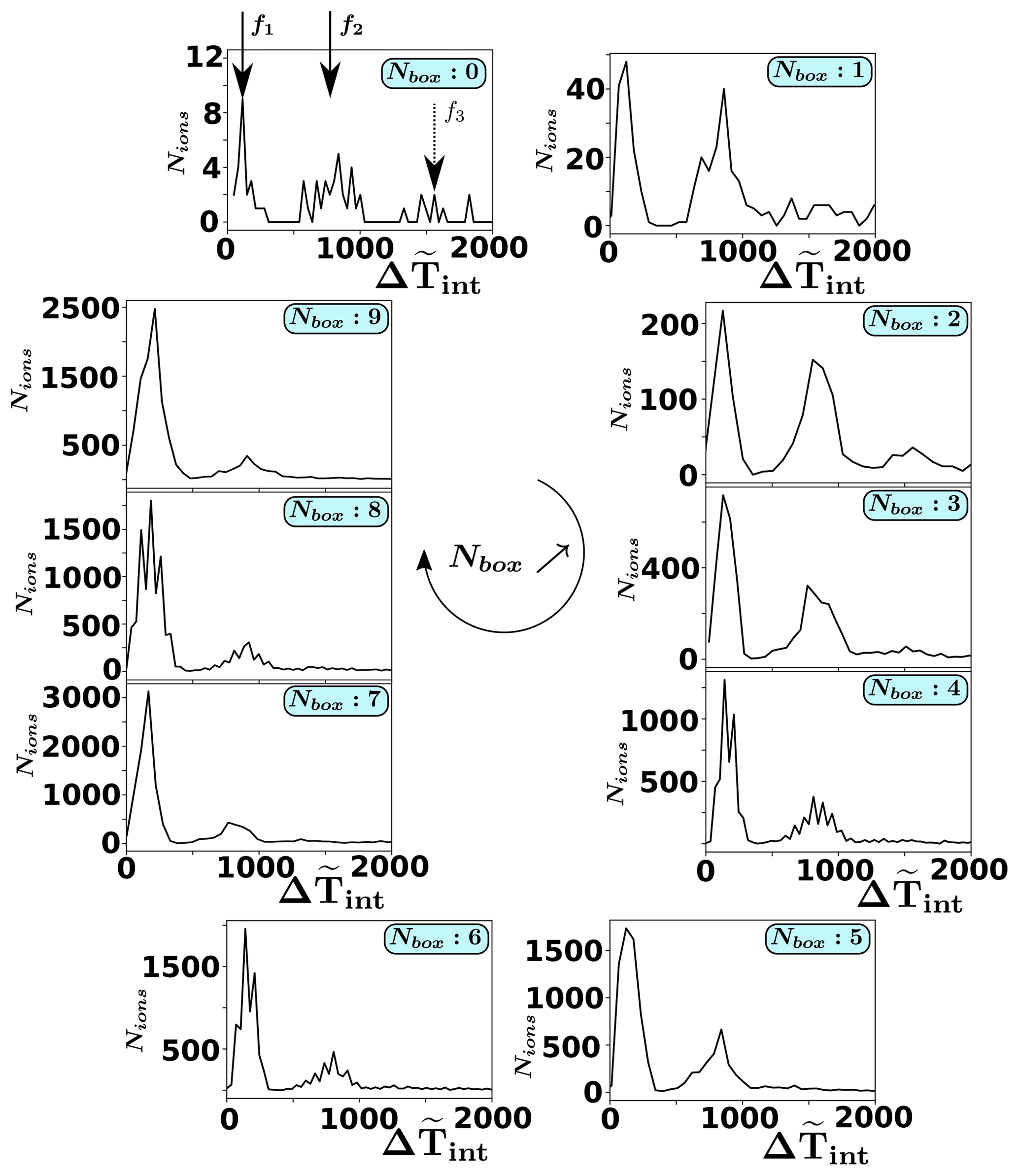
Figure 5 FCE configuration: plots of the ion distribution function (for each box $N_{\mathrm{Box}}=\mathrm{0}-\mathrm{9}$) versus the interaction time range $\mathrm{\Delta }{\stackrel{\mathrm{̃}}{T}}_{\mathrm{int}}$ spent by each particle within the shock front. As shown, this interaction time range is not continuous, but it evidences distinct bursts of reflected ions (hereafter named f₁ and f₂), respectively, defined at $\mathrm{\Delta }{\stackrel{\mathrm{̃}}{T}}_{\mathrm{int}}\approx \mathrm{250}\approx \mathrm{0.25}{\stackrel{\mathrm{̃}}{\mathit{\tau }}}_{\mathrm{ci}}$ and $\mathrm{\Delta }{\stackrel{\mathrm{̃}}{T}}_{\mathrm{int}}\approx \mathrm{950}\approx \mathrm{1}{\stackrel{\mathrm{̃}}{\mathit{\tau }}}_{\mathrm{ci}}$, where ${\stackrel{\mathrm{̃}}{\mathit{\tau }}}_{\mathrm{ci}}$ is the upstream cyclotronic period. A third burst f₃ of reflected ions can be identified around $\mathrm{\Delta }{\stackrel{\mathrm{̃}}{T}}_{\mathrm{int}}\approx \mathrm{1500}\approx \mathrm{1.5}{\stackrel{\mathrm{̃}}{\mathit{\tau }}}_{\mathrm{ci}}$ for $N_{\mathrm{Box}}=\mathrm{0}-\mathrm{2}$ but can be neglected as compared with the others.

Third, in order to complete information deduced from Fig. 4, Fig. 5 plots the number of reflected ions versus the time spent within the shock front. This interaction time $\mathrm{\Delta }{\stackrel{\mathrm{̃}}{T}}_{\mathrm{int}}$ is defined as the time difference between the time associated to ${\mathit{\theta }}_{\mathrm{Bn}}^{\mathrm{exit}}$ and to ${\mathit{\theta }}_{\mathrm{Bn}}^{\mathrm{hit}}$. Different main maxima of back-streaming ions' density are evidenced, namely f₁, f₂; a third maximum f₃ can be also observed for boxes N_Box=0–4, but its amplitude is too weak to be relevant in this discussion. One important feature is that f₁ and f₂ appear in all boxes and are independent of the box number. More precisely, f₁ appears about $\mathrm{\Delta }{\stackrel{\mathrm{̃}}{T}}_{\mathrm{int}}\approx \mathrm{0.25}{\stackrel{\mathrm{̃}}{\mathit{\tau }}}_{\mathrm{ci}}\approx {\stackrel{\mathrm{̃}}{\mathit{\tau }}}_{\mathrm{ci}}^{\mathrm{shock}}$ while f₂ is observed at $\mathrm{\Delta }{\stackrel{\mathrm{̃}}{T}}_{\mathrm{int}}\approx \mathrm{1}{\stackrel{\mathrm{̃}}{\mathit{\tau }}}_{\mathrm{ci}}\approx \mathrm{4}{\stackrel{\mathrm{̃}}{\mathit{\tau }}}_{\mathrm{ci}}^{\mathrm{shock}}$, where ${\stackrel{\mathrm{̃}}{\mathit{\tau }}}_{\mathrm{ci}}^{\mathrm{shock}}$ is the local gyroperiod estimated within the shock front (at the middle of the ramp). This indicates that the reflection process is not uniform in time but leads to the formation of ion bursts associated to the shock dynamics, even if the number of ions which spend several gyroperiods ${\stackrel{\mathrm{̃}}{\mathit{\tau }}}_{\mathrm{ci}}^{\mathrm{shock}}$ (i.e., ≈4 bounces) within the shock front is rapidly negligible. In addition, for N_Box=0–2, f₁ and f₂ have a similar amplitude, which is not the case for N_Box=4–9. In fact, a close look at f₁ and f₂ shows that f₂ does not decrease in magnitude but rather the amplitude of f₁ drastically increases from 10 (N_Box=0) to 2500 (N_Box=9). Then, the f₂ population is always present but becomes negligible for lower θ_Bn as compared with f₁; this explains why we do not observe two distinct spots for N_Box=4–9.

One helpful aspect of the test particle approach is including or excluding some electromagnetic field components in order to analyze their impact on the particles dynamics. Indeed, it is clear that some electric field component (i.e., E_l×B drift) and strong magnetic gradients drift (i.e., $\propto -\mathbf{\nabla }B\times \mathit{B}$ drift) can be a prerequisite for a large drift along the front (i.e., ${\mathrm{\Delta }}_{\mathrm{int}}{\mathit{\theta }}_{\mathrm{Bn}}\approx \mathrm{15}{}^{\circ }$), whereas it could be unnecessary for the other case Δ_intθ_Bn≈4–5^∘. Unfortunately, the shock front magnetic gradient cannot be canceled without the shock itself; then, we will focus our study by including or excluding the electric components which will shed new light on the origin of back-streaming ions filling the foreshock.

3.2 Impact of electric field components

Savoini and Lembège (2015) have analyzed the impact of E×B drift velocity on the dynamics of back-streaming ions (Gurgiolo et al., 1983) and, more particularly, as a source of FAB and/or GPB populations. This study has shown that the origin of both populations can be easily explained in terms of E×B drift associated or not to a diffusion in the velocity space, but it was not able to explain the details of the reflection mechanism itself. Then, herein, we will focus on the role of the electrostatic field component ${\stackrel{\mathrm{̃}}{E}}_{\mathrm{l}}$ built up within the shock front (i.e., space charge effects). This longitudinal component, defined along the normal to the shock front, can be associated to the electrostatic potential wall responsible for some reflected ions. In the case of a constant shock profile in time with a planar geometry, this reflection does conserve the energy since the potential is the same before and after the reflection, and the total work of the electric force is canceled. Nevertheless, in more realistic conditions, this scenario is not valid anymore for ions which drift along the shock front and suffer both time and space electric and magnetic field variations. Then, in the following sections, we will preferentially use the field E_l rather than the potential Φ.

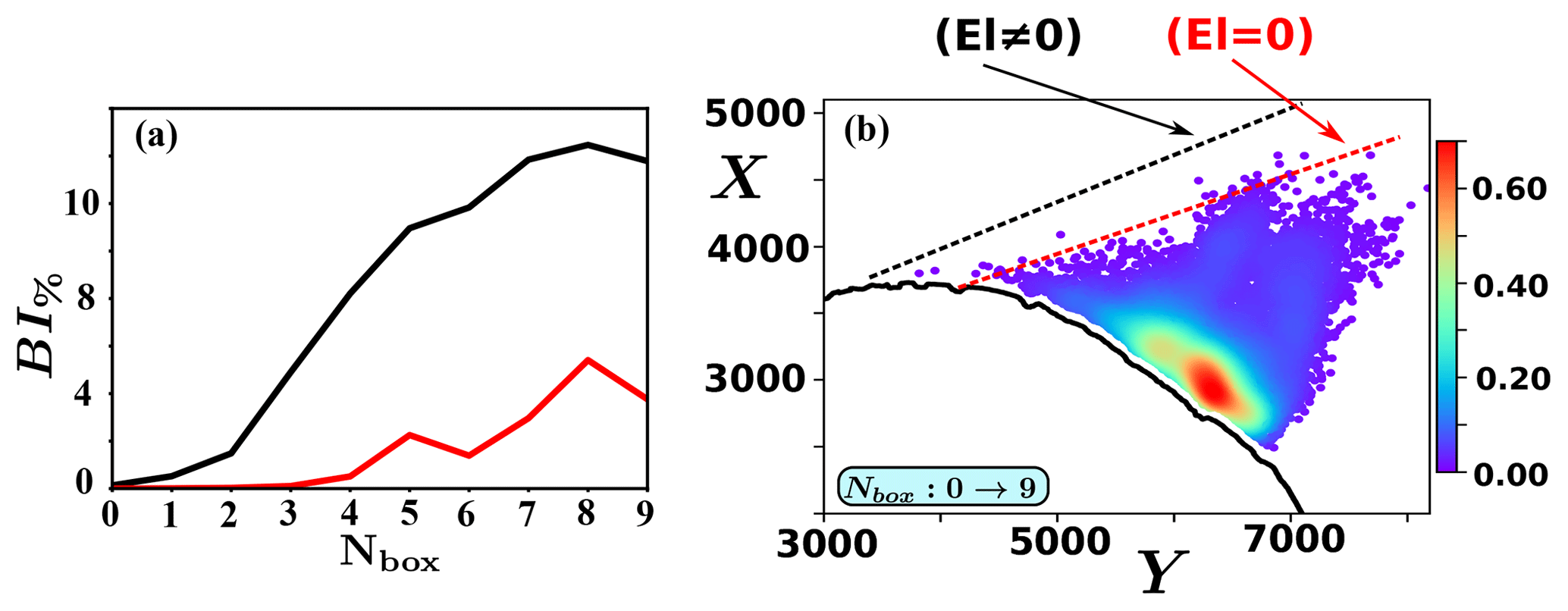
Figure 6 FCE configuration: characteristics of the ion foreshock with and without the electrostatic field component ${\stackrel{\mathrm{̃}}{E}}_{\mathrm{l}}$ (i.e., ${\stackrel{\mathrm{̃}}{E}}_{\mathrm{l}x}={\stackrel{\mathrm{̃}}{E}}_{\mathrm{l}y}=\mathrm{0}$). Panel (a) shows the percentage of the back-streaming ions BI_% versus the box number. Black and red lines are defined for ${\stackrel{\mathrm{̃}}{E}}_{\mathrm{l}}\ne \mathrm{0}$ and ${\stackrel{\mathrm{̃}}{E}}_{\mathrm{l}}=\mathrm{0}$, respectively. Panel (b) shows the density of the back-streaming particles in the same format as Fig. 3 but when ${\stackrel{\mathrm{̃}}{E}}_{\mathrm{l}}=\mathrm{0}$. Only the view which aggregates all boxes (i.e., N_Box=10) is shown in order to evidence the location of the edge of the ion foreshock (dotted line) in each case.

Figure 6a shows the percentage BI_% of back-streaming ions versus the box number where the black and red curves are defined for ${\stackrel{\mathrm{̃}}{E}}_{\mathrm{l}}\ne \mathrm{0}$ and ${\stackrel{\mathrm{̃}}{E}}_{\mathrm{l}}=\mathrm{0}$ respectively. The impact of the ${\stackrel{\mathrm{̃}}{E}}_{\mathrm{l}}$ field (i.e., the potential wall) on the reflection process is clearly apparent for all θ_Bn values (namely for each N_Box number). In particular, the percentage BI_% strongly decreases as ${\stackrel{\mathrm{̃}}{E}}_{\mathrm{l}}=\mathrm{0}$, which illustrates the dominant role of ${\stackrel{\mathrm{̃}}{E}}_{\mathrm{l}}$ field whatever the box is. This is especially true for the lower box number N_Box=0–3 (i.e., high θ_Bn approaches 90^∘) where very few back-streaming ions are observed. This point is not surprising if one remembers that this electrostatic field decelerates the incoming ions (i.e., accelerates ions in the present reference frame) and contributes to the reflection process. In other words, for N_Box=0 (i.e., largest θ_Bn), escaping ions have to be accelerated to higher parallel velocity, as reviewed in Burgess et al. (2012). Let us stress that Fig. 6a exhibits a clear change in the slope of BI_% increase at the box N_Box=2 centered around ${\mathit{\theta }}_{\mathrm{Bn}}=\mathrm{70}{}^{\circ }$. Herein, we will consider this value as the reference angle identifying the starting location of the ion foreshock edge attached to the shock front. This value is in reasonable agreement with the value (${\mathit{\theta }}_{\mathrm{io},\mathrm{fore}}\approx \mathrm{66}{}^{\circ }$) found approximately in the previous self-consistent PIC simulations Savoini and Lembège (2015).

Another consequence is illustrated in Fig. 6b, which shows that the edge of the ion foreshock is shifted due to the lack of reflected ions, and it starts around ${\mathit{\theta }}_{\mathrm{Bn}}\approx \mathrm{55}{}^{\circ }$. Clearly, the contribution of the electric field is important for ions which populate the edge of the foreshock and need to escape at high θ_Bn.

Another way to observe the strong impact of ${\stackrel{\mathrm{̃}}{E}}_{\mathrm{l}}$ on the dynamics of reflected ions is illustrated in Fig. 7, which shows the two ${\mathit{\theta }}_{\mathrm{Bn}}^{\mathrm{hit}}$ and ${\mathit{\theta }}_{\mathrm{Bn}}^{\mathrm{exit}}$ distributions in the same format as that of Fig. 4. The number of back-streaming ions decreases drastically for all boxes and is zero for N_Box=0. Furthermore, the density is not uniform for all boxes and appears to be much more important for N_Box=5–9 than for N_Box=1–4. The ${\mathit{\theta }}_{\mathrm{Bn}}^{\mathrm{exit}}$ distribution is strongly modified and a comparison between Figs. 4 and 7 can be summarized as follows:

1. The boxes N_Box=1–2 evidence a total absence of reflected ions with a small range Δ_intθ_Bn, and only the ${\mathit{\theta }}_{\mathrm{Bn}}^{\mathrm{exit}}$ distribution around 60^∘ persists. This result shows that ${\stackrel{\mathrm{̃}}{E}}_{\mathrm{l}}$ field plays a key role, more specifically on back-streaming ions suffering a one bounce reflection near the edge of the ion foreshock (i.e., Δ_intθ_Bn≈4–5^∘).

2. The ${\mathit{\theta }}_{\mathrm{Bn}}^{\mathrm{exit}}$ distribution in both cases (${\stackrel{\mathrm{̃}}{E}}_{\mathrm{l}}\ne \mathrm{0}$ in Fig. 4 and ${\stackrel{\mathrm{̃}}{E}}_{\mathrm{l}}=\mathrm{0}$ in Fig. 7) is roughly similar in corresponding boxes for all N_Box≥6. This can be interpreted as either that the ions have been accelerated enough during their reflection at the shock front or that they need a lower parallel velocity to escape upstream. As a consequence, the E_l component is not mandatory anymore, and the mirror magnetic mechanism at the shock front can be invoked as the only reflection process.

In summary, the comparison between Figs. 4 and 7 evidences that ${\stackrel{\mathrm{̃}}{E}}_{\mathrm{l}}$ components are essential in the ion reflection for a high θ_Bn angle ($>\mathrm{56}{}^{\circ }$, i.e., N_Box=6–9) where ions need a strong acceleration process but play a less important role at lower θ_Bn angles. Conversely, for N_Box=6–9, the reflection process takes place with a very small Δ_intθ_Bn, with or without the electric field. In other words, the large shock drift invoked for ${\mathit{\theta }}_{\mathrm{Bn}}\le \mathrm{56}{}^{\circ }$ seems to be mainly supported by the convective electric field ${\stackrel{\mathrm{̃}}{E}}_{\mathrm{t}}$ components present at the shock front.

Similarly, the one bounce reflection always occurs, even in the absence of ${\stackrel{\mathrm{̃}}{E}}_{\mathrm{l}}$ field (i.e., in the absence of the shock front potential wall), and can then be associated to a magnetic reflection which seems to be very efficient, especially at lower θ_Bn. This one bounce reflection (i.e., f₁) corresponds essentially to a short interaction time, as illustrated in Fig. 5 ($\mathrm{\Delta }{\stackrel{\mathrm{̃}}{T}}_{\mathrm{int}}\approx \mathrm{1}{\stackrel{\mathrm{̃}}{\mathit{\tau }}}_{\mathrm{ci}}^{\mathrm{shock}}$). Then, the ion energy gain is essentially due to a Fermi-type acceleration.

Figure 7 FCE configuration: same plots as for Fig. 4 but when electrostatic field components E_lx and E_ly are artificially excluded (E_l=0). The angles ${\mathit{\theta }}_{\mathrm{Bn}}^{\mathrm{hit}}$ and ${\mathit{\theta }}_{\mathrm{Bn}}^{\mathrm{exit}}$ have been reported in N_Box=2 for reference purposes.

3.3 Impact of the shock front nonstationarity

Previous studies have largely evidenced that a quasi-perpendicular shock front can be intrinsically nonstationary due to different mechanisms (for a review, see Lembège et al., 2004; Marcowith et al., 2016). Then, it is important to analyze the impact of such nonstationarity on the temporal ion foreshock dynamics. As a first step, we plot in Figure 8 the time evolution of the back-streaming ions' percentage BI_% as these leave the front and escape into the upstream region, where BI_% is the instantaneous rate computed during a short time range $\mathrm{\Delta }\stackrel{\mathrm{̃}}{T}={\stackrel{\mathrm{̃}}{\mathit{\tau }}}_{\mathrm{ci}}/\mathrm{20}$. The time ${\stackrel{\mathrm{̃}}{T}}_{\mathrm{init}}=\mathrm{1248}$ is the initial time when test particles are launched into the time-dependent simulation.

Figure 8 FCE configuration: time history of the reflected ion percentage BI_%; each value is computed during a short integrated time interval $\mathrm{\Delta }\stackrel{\mathrm{̃}}{T}={\stackrel{\mathrm{̃}}{\mathit{\tau }}}_{\mathrm{ci}}/\mathrm{20}$ for the different boxes. Within this interval, only the newly reflected ions are memorized. As for Fig. 6, black and red lines correspond to the case where the electric field is included (${\stackrel{\mathrm{̃}}{E}}_{\mathrm{l}}\ne \mathrm{0}$) or excluded (${\stackrel{\mathrm{̃}}{E}}_{\mathrm{l}}=\mathrm{0}$), respectively. We have used the same normalization in order to compare both cases. The blue dotted straight lines are not obtained from a data linear approximation but only indicate the mean values of the time modulations.

• i.

  Results of Fig. 8 are obtained as the ${\stackrel{\mathrm{̃}}{E}}_{\mathrm{l}}$ field components are included (black curve) and artificially excluded (red curve). One concludes that the percentage BI_% strongly decreases as ${\stackrel{\mathrm{̃}}{E}}_{\mathrm{l}}$ components are excluded, and that the impact of ${\stackrel{\mathrm{̃}}{E}}_{\mathrm{l}}$ field is emphasized for lower N_Box. In other words, the back-streaming ions mainly appear for higher N_Box>5 (i.e., for lower θ_Bn), even in absence of ${\stackrel{\mathrm{̃}}{E}}_{\mathrm{l}}$ field.

• ii.

  The different results may be classified into two groups, where (i) the first one concerns boxes N_Box=0–4 showing a slow increase (almost monotonic) in the reflection rate and (ii) a second group N_Box=5–9 evidences a steep increase followed by a flat-top shape around BI_%≈1, even if it increases slightly with N_Box. At the end of the simulation, the strong decrease in BI_% observed for all boxes corresponds to the time when all ions of the different boxes have been swapped by the propagating shock front and then no more ions are back streaming.

  For the first group N_Box=0–4, a delay is observed in the formation of back-streaming ions between the different boxes, although test particles are initially evenly distributed in the whole boxes. For N_Box=0, back-streaming ions appear around $\stackrel{\mathrm{̃}}{T}\approx \mathrm{5248}$, i.e., well after the initial release time ${\stackrel{\mathrm{̃}}{T}}_{\mathrm{init}}=\mathrm{1248}$ (i.e., $\mathrm{\Delta }\stackrel{\mathrm{̃}}{T}=\mathrm{5248}-\mathrm{1248}$, which covers $\approx \mathrm{2.6}{\stackrel{\mathrm{̃}}{\mathit{\tau }}}_{\mathrm{ci}}$), whereas this time delay decreases to $\stackrel{\mathrm{̃}}{T}\approx \mathrm{2018}$ (i.e., $\mathrm{\Delta }\stackrel{\mathrm{̃}}{T}=\mathrm{2018}-\mathrm{1248}=\mathrm{770}$, which covers $\approx \mathrm{0.5}{\stackrel{\mathrm{̃}}{\mathit{\tau }}}_{\mathrm{ci}}$) as N_Box increases. This illustrates the larger time delay of ions having interacted with the front to escape upstream at high θ_Bn. For N_Box=0–2, ions have to stay longer within the shock front to finally escape at lower ${\mathit{\theta }}_{\mathrm{Bn}}^{\mathrm{exit}}$ (Fig. 7), which is illustrated by the increase of BI_% as the time evolves (Fig. 8). The second group (N_Box=5–9) concerns boxes which are already at a lower angle θ_Bn with easier escaping conditions. In this case, ions are reflected continuously with some time variation in BI_%.

• iii.

  Another interesting feature is the presence of different modulations which are superimposed on a time-averaged reflection ion rate (blue dashed line), especially for the boxes N_Box=1–5 and the boxes N_Box=7–8. Nearly all boxes exhibit these modulations which represent about 40 % of the averaged BI_%, although the amplitude of these modulations varies versus time and N_Box. These evidence a nonstationary ion escaping rate. These modulations almost disappear in the case of ${\stackrel{\mathrm{̃}}{E}}_{\mathrm{l}}=\mathrm{0}$ (red line). This illustrates that the presence of the ${\stackrel{\mathrm{̃}}{E}}_{\mathrm{l}}$ field component is a key ingredient in the formation of these modulations since this electric field component is also involved in the shock front self-reformation, as described in previous works (Lembège and Savoini, 1992; Scholer et al., 2003; Matsukiyo and Scholer, 2006).

  This result confirms the importance of the electrostatic field component at the shock front in the reflection processes of the back-streaming ions and, most importantly, on the ion foreshock nonstationarity behavior as described in a previous paper (Savoini and Lembège, 2015). Nevertheless, it is quite difficult to establish a one-to-one correspondence between these modulations and the nonstationarity of the shock front because, during the sampling time interval $\mathrm{\Delta }\stackrel{\mathrm{̃}}{T}={\stackrel{\mathrm{̃}}{\mathit{\tau }}}_{\mathrm{ci}}/\mathrm{20}$, the front nonstationarity and the time-of-flight effects have mixed ions coming from either different times and/or different ${\mathit{\theta }}_{\mathrm{Bn}}^{\mathrm{exit}}$ regions (even if they are in the same box). So this self-consistent approach is not totally adapted to resolve this question. A complementary approach is necessary, based on simplified simulations with fixed shock front profiles in expansion (nonstationary effects are excluded). This motivates the homothetic expansion model (HE) described in the next section.

4 Numerical results: the homothetic expansion (HE) model

4.1 Descriptions of the HE model

Let remember that all simulations are made in the solar wind reference frame (i.e., the curved shock expands into the upstream region where the solar wind is at rest). As a consequence, if one follows test particles within this configuration, we have to mimic this behavior. In order to proceed, we apply a homothetic transformation (homogeneous dilatation in all directions) with an expansion factor deduced from the shock front velocity determined at selected times, as illustrated in panels 3a–b of Fig. 1. Special attention has been taken in the determination of this homothetic factor $\mathit{\lambda }=v_{\mathrm{shock}}\times t$, since the shock front velocity v_shock at a given time must fit with the corresponding value issued from the PIC simulations (Savoini and Lembège, 2015). With this information, we are able to expand the shock front through a cubic interpolation as it propagates with v_shock in an expanding simulation plane (i.e., the grid cells stay constant ${\stackrel{\mathrm{̃}}{\mathrm{\Delta }}}_x={\stackrel{\mathrm{̃}}{\mathrm{\Delta }}}_y=cte$ but the number of the grid cells increases accordingly). In other words, all points of electromagnetic fields at the shock front follow the relation $\mathit{O}\mathit{M}⟼(v_{\mathrm{shock}}\times t)\mathit{O}\mathit{M}$, where v_shock is the value of the shock velocity, as computed from our self-consistent 2D PIC simulations at the selected time, and OM is the vector between the initial location of the shock front (i.e., the point O) and any point of the field array (i.e., the point M). At this stage, we have to point out that the velocity v_shock remains artificially constant during the whole simulation, which is not the case for the FCE model where v_shock slightly decreases. Then, the same procedure is repeated for another selected time, so that one can analyze the impact of different shock front inhomogeneities and curvature on ion dynamics; let us note that time-of-flight effects are always included. Each front profile is analyzed within a similar simulation time range $\approx \mathrm{3}{\stackrel{\mathrm{̃}}{\mathit{\tau }}}_{\mathrm{ci}}$. In summary, similar simulations are performed for 174 different times in order to simulate all the different shock profiles provided by the 2D PIC self-consistent simulation from ${\stackrel{\mathrm{̃}}{t}}_{\mathrm{init}}=\mathrm{1.2}{\stackrel{\mathrm{̃}}{\mathit{\tau }}}_{\mathrm{ci}}$ to ${\stackrel{\mathrm{̃}}{t}}_{\mathrm{simul}}=\mathrm{5.4}{\stackrel{\mathrm{̃}}{\mathit{\tau }}}_{\mathrm{ci}}$.

4.2 General features of the back-streaming ions

Figure 9 has been achieved in the same format as Fig. 8 by performing 100 independent simulations (i.e., we take only the first 100 simulations so that all test particles hit the propagating shock front). During this range, the shock front is forced to expand (see Sect. 4.1). For example, the chosen time $\stackrel{\mathrm{̃}}{T}=\mathrm{4456}\approx \mathrm{4.2}{\stackrel{\mathrm{̃}}{\mathit{\tau }}}_{\mathrm{ci}}$ on the abscissa axis corresponds to one particular shock front profile (i.e., including all electromagnetic field components issued from the previous self-consistent PIC simulations) from which we have measured the instantaneous shock front velocity and that we follow during the time range covering $\approx \mathrm{3}{\stackrel{\mathrm{̃}}{\mathit{\tau }}}_{\mathrm{ci}}$.

The purpose is to determine (i) whether some shock profiles are more appropriate than others for the formation of back-streaming ions and (ii) if, yes, whether better reflection takes place for some particular angular range of θ_Bn.

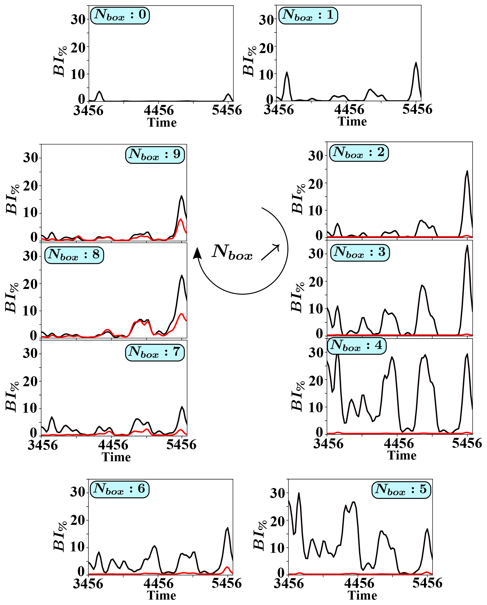
Figure 9 HE configuration: percentage BI_% of back-streaming ions measured at the end of each simulation, where each time corresponds to a given fixed shock front. For each shock profile in homothetic expansion, the simulation covers $\mathrm{3}{\stackrel{\mathrm{̃}}{\mathit{\tau }}}_{\mathrm{ci}}$, allowing one to obtain a well-developed ion foreshock, and BI_% represents the ratio of the back-streaming ions over the total number of upstream ions which are released at the beginning of the simulation within a given box. As in Fig. 7, black and red lines correspond to the case when the E_l field is included and artificially excluded, respectively. The concerned shock profiles are chosen only at late times of the full PIC simulation (from $\stackrel{\mathrm{̃}}{T}=\mathrm{3456}$ to 5474), where the curvature radius of the shock front is relatively large ($\stackrel{\mathrm{̃}}{R}>\mathrm{70}{\stackrel{\mathrm{̃}}{\mathit{\rho }}}_{\mathrm{ci}}$).

The comparison of Figs. 8 and 9 provides the following information. The maximum BI_% value is much higher for the HE model than for the previous FCE model for each corresponding box. For example, for N_Box=9, BI${}_{\mathit{\%}}^{\max }\approx \mathrm{1.2}$ in the FCE simulations as compared with BI${}_{\mathit{\%}}^{\max }\approx \mathrm{15}$ in the HE configuration. In fact, one has to remember that for the FCE model the BI${}_{\mathit{\%}}^{\max }$ value represents an instantaneous reflection rate versus the shock front evolution, whereas this rate is a time-integrated value for the HE model. Indeed, in this model, the shock front profile stays the same during the whole simulation, and then, if this profile allows the reflection of some incident ions, they will be reflected continuously, leading to a high BI_% number.

Obviously, the main information is not the BI_% value itself but rather its evolution versus time and for different shock profiles. Other main results issued from Fig. 9 may be summarized as follows:

1. The N_Box=0 box evidences almost no reflection for the majority of the shock front profiles, which indicates that nonstationarity effects present in the FCE configuration (i.e., Fig. 3) are needed for feeding back-streaming ions along the edge of the foreshock.

2. Boxes N_Box=1–8 clearly show some strong modulations in the percentage BI_% versus the shock profile of concern, which corresponds to a quasi-periodic bursty emission of back-streaming ions. The BI_% rate periodically reaches a maximum value followed by a minimum around zero. The corresponding time period $\mathrm{\Delta }{\stackrel{\mathrm{̃}}{T}}_{\max }$ is about $\approx \mathrm{460}=\mathrm{0.5}{\stackrel{\mathrm{̃}}{\mathit{\tau }}}_{\mathrm{ci}}$ (between two successive maxima). The temporal width of each maximum is about $\mathrm{\Delta }{\stackrel{\mathrm{̃}}{T}}_{\mathrm{range}}\approx \mathrm{256}=\mathrm{0.25}{\stackrel{\mathrm{̃}}{\mathit{\tau }}}_{\mathrm{ci}}$. These modulations mean that conditions for the formation of back-streaming particles are not continuous but correspond to some specific shock front profiles. In addition, these modulations appear synchronized in time for the different boxes 1–7, which implies that the local reflection conditions are not strongly dependent on the θ_Bn angle but rather depend on the shock profile at certain times.

3. In contrast, the boxes N_Box=8–9 also evidence the same kind of modulations but with greatly reduced amplitude; these are even nonexistent between $\stackrel{\mathrm{̃}}{T}\approx \mathrm{3456}$ and 4456, which indicates a low sensitivity to the shock front profile when approaching ${\mathit{\theta }}_{\mathrm{Bn}}=\mathrm{45}{}^{\circ }$.

4. Similarly, the maximum values BI${}_{\mathit{\%}}^{\max }$ (black curve) change drastically with box numbers, namely from small amplitudes, BI_%≤6 for N_Box=1–2, to very high values, BI_%≈30 for N_Box=3–5, before decreasing again for N_Box=6–9. These variations may be understood by taking into account the reflection processes present at these different θ_Bn and, more specifically, in regards to the electric field components. For boxes N_Box=0–2, reflection is almost impossible without the ${\stackrel{\mathrm{̃}}{E}}_{\mathrm{l}}$ component (i.e., electric potential wall). As θ_Bn decreases (for N_Box=3–5), the reflection becomes easier and both magnetic and electric fields contribute to the percentage of reflected ions. Finally, for the last boxes N_Box=6–9, the peak amplitude decreases but the contribution of ${\stackrel{\mathrm{̃}}{E}}_{\mathrm{l}}$ becomes less important in the reflection process, as evidenced by comparing both black (${\stackrel{\mathrm{̃}}{E}}_{\mathrm{l}}\ne \mathrm{0}$) and red (${\stackrel{\mathrm{̃}}{E}}_{\mathrm{l}}=\mathrm{0}$) curves. Instead, another process, essentially driven by the magnetic field (mirror reflection) contributes more since the peak amplitude of the red curve increases progressively as N_Box increases from 6 to 9.

5. Only the last peak around $\stackrel{\mathrm{̃}}{T}\approx \mathrm{5456}$ has a different behavior in comparison with others. In particular, we observe that, for these different times or profiles, the presence of the ${\stackrel{\mathrm{̃}}{E}}_{\mathrm{l}}$ leads to higher BI_%. This behavior can be understood because v_shock is lower for these times, and the ${\stackrel{\mathrm{̃}}{E}}_{\mathrm{l}}$ component is necessary for decelerating ions and reflecting them. Without this component, only the magnetic reflection is present, and BI_% has the same amplitude as the previous maximum.

6. Finally, Fig. 9 confirms the key role of E_l field in back-streaming ion formation, except when approaching ${\mathit{\theta }}_{\mathrm{Bn}}=\mathrm{45}{}^{\circ }$ (N_Box=8–9) while another reflection process is also at work (in absence of E_l). This represents an indirect way of stressing the noticeable impact of the magnetic field in this angular range. This magnetic reflection process is more evidenced at lower θ_Bn since ions need less parallel velocity to be reflected back into the upstream region. This statement can be quantified more precisely, as explained in Sect. 5.

This result is an illustration of the impact of the electrostatic component at the shock front. As is well known, this component works to decelerate incoming ions (i.e., accelerate in our solar wind frame) and to accelerate electrons (i.e., decelerate in our solar wind frame) to the downstream region (Savoini and Lembège, 1994; Bale et al., 2005). As a consequence, this electrostatic component is an essential ingredient in the formation of back-streaming ions, especially at higher θ_Bn.

5 Discussions

A previous paper (Savoini and Lembège, 2015) demonstrated that all reflected ions suffered the same E×B drift in the velocity space, which can account for the pitch angle distributions observed at the shock front. In fact, the key point is the time spent by particles within the front shock, which finally decides whether ions will escape to form the FAB (with a pitch angle $\mathit{\alpha }\approx \mathrm{0}{}^{\circ }$) or GPB populations (with a pitch angle $\mathit{\alpha }\ne \mathrm{0}{}^{\circ }$), where α is the angle between the velocity vector and the magnetic field. In other words, the FAB population may be associated to a large drift along the shock front (and/or long interaction time) during which particles see a time-varying shock front and lose their phase coherency; this case corresponds to a large angular range Δ_intθ_Bn mentioned in Sect. 3.1. In contrast, the ions of the GPB population have a shorter interaction time with the shock front associated to a small angular range Δ_intθ_Bn. Present test particle simulations allow one to have a deeper insight to the spatial origin of the observed FAB and GPB populations. Then, we have to analyze the ion velocity distribution more carefully.

Figure 10 plots the local perpendicular velocity distribution functions $f({\mathit{v}}_{⟂\mathrm{1}},{\mathit{v}}_{⟂\mathrm{2}})$ in both FCE and HE approaches (where v_⟂1 and v_⟂2 refer the ion perpendicular velocity components defined with respect to the local magnetic field). All plots are obtained at the end of the simulations and take into account the different populations observed in Figs. 4 and 7 (i.e., both distinct peaks of ${\mathit{\theta }}_{\mathrm{Bn}}^{\mathrm{exit}}$ angle for lower N_Box are included); results issued from FCE (Fig. 10, left panel) and HE (Fig. 10, right panel) configurations are considered. For the HE configuration, we chose an initial time $\stackrel{\mathrm{̃}}{T}=\mathrm{4848}$ (see Fig. 9 for reference) which corresponds to a maximum of BI_% in order to have enough reflected ions in the velocity space. Results from the three different boxes, $N_{\mathrm{Box}}=\mathrm{1},\mathrm{4}$ and 8, are represented in order to give an overview of the whole ion foreshock components.

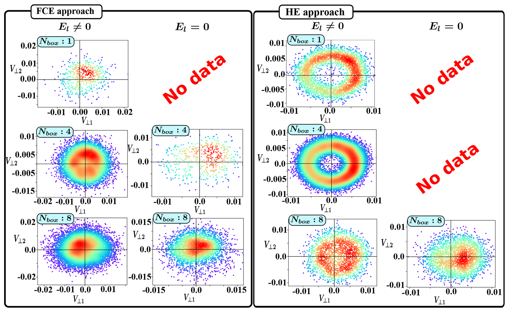
Figure 10 Local perpendicular ion velocity space (v_⟂1, v_⟂2) of all back-streaming ions computed at the end time of the simulations (i.e., after 3τ_ci for all simulations) for boxes $N_{\mathrm{Box}}=\mathrm{1},\mathrm{4}$ and 8 in the FCE approach when the ${\stackrel{\mathrm{̃}}{E}}_{\mathrm{l}}$ is included (left panel); the case ${\stackrel{\mathrm{̃}}{E}}_{\mathrm{l}}=\mathrm{0}$ is not plotted since the percentage BI_% is very weak (see Fig. 8). The right panel shows similar results for the same boxes in the HE configuration (corresponding to $\stackrel{\mathrm{̃}}{T}=\mathrm{4848}$) in both cases where ${\stackrel{\mathrm{̃}}{E}}_{\mathrm{l}}$ is included and artificially excluded; statistical results where BI_% is too weak are not shown. Red and blue hold for maximum and minimum density value in the velocity space.

Results of the FCE configuration (left panels) can be analyzed in Figs. 4, 7 and 10. Plots of the E_l≠0 case (Fig. 10) show that the N_Box=1 has a low number of upstream reflected ions, which leads to poor statistics and a noisy $f({\mathit{v}}_{⟂\mathrm{1}},{\mathit{v}}_{⟂\mathrm{2}})$ distribution. Nevertheless, it evidences approximately a distribution with a maximum slightly noncentered at ${\mathit{v}}_{⟂}=\mathrm{0}$. Then, this distribution can be viewed as a mixing of GPB and FAB populations, even if the GPB population with a pitch angle different zero is the largest one. When moving further into the foreshock region (i.e., lower θ_Bn angle with N_Box=4), the number of reflected ions drastically increases and we observe more clearly the characteristic partial ring of the GPB population (as in Savoini and Lembège, 2015). In addition, the center of the ring is also partially filled in because of partial diffusion due to particles having a large Δ_intθ_Bn range, corresponding to the ${\mathit{\theta }}_{\mathrm{Bn}}^{\mathrm{exit}}$ peak around 60^∘ in Fig. 4, and/or by the intrinsic time fluctuations of the front which tends to blur out the velocity distribution both in perpendicular and parallel directions. At last, in agreement with the associated small ${\mathit{\theta }}_{\mathrm{Bn}}^{\mathrm{exit}}$ of Fig. 4, N_Box=8 (in Fig. 10) also evidences a non-Maxwellian-like distribution ($\mathit{\alpha }\ne \mathrm{0}{}^{\circ }$). When we look at the E_l=0 case, we observe roughly the same behavior for all boxes, even if the decrease in the back-streaming ions number in box N_Box=8 makes the comparison difficult.

A further analysis requires a similar approach with the HE configuration in which we follow a succession of independent expanding shock profiles in order to exclude the impact of the time fluctuations on the velocity distribution $f({\mathit{v}}_{\parallel },{\mathit{v}}_{⟂})$; then, no ion diffusion associated to these fluctuations is allowed. Results of the HE configuration (right panel, Fig. 10) show reflected ions for N_Box=1 when ${\stackrel{\mathrm{̃}}{E}}_{\mathrm{l}}\ne \mathrm{0}$, but once again, no reflected ions can be seen when ${\stackrel{\mathrm{̃}}{E}}_{\mathrm{l}}=\mathrm{0}$. This evidences the importance of the electrostatic potential wall in order to reflect upstream ions for high θ_Bn. On the other hand, if the amplitude of the perpendicular velocity is roughly the same for the two different configurations (FCE and HE), the HE case shows a very well-formed ring, in contrast with the FCE case, which exhibits a diffuse velocity space. This illustrates that field time variations (FCE configuration) are much more efficient at diffusing particles than the fields spatial variations (HE configuration). Similarly, N_Box=4 exhibits a clear ring, which is a feature of the GPB population. The center of the ring is not partially filled in since time velocity diffusion is excluded. These results demonstrate that the formation of the FAB-like population is also mainly due to ion velocity diffusion related to the time fluctuations of the shock front which can have different origins, as described in previous works (Kucharek et al., 2004; Bale et al., 2005). Finally, for N_Box=8, the velocity distribution drastically changes from a ring (${\stackrel{\mathrm{̃}}{E}}_{\mathrm{l}}\ne \mathrm{0}$) to a localized bump (${\stackrel{\mathrm{̃}}{E}}_{\mathrm{l}}=\mathrm{0}$) roughly similar to the FCE case. It is clear that the number of reflected ions decreases drastically as ${\stackrel{\mathrm{̃}}{E}}_{\mathrm{l}}$ field components are artificially suppressed. But, more important is that the formation of a nongyrotropic distribution does not depend strongly on the ${\stackrel{\mathrm{̃}}{E}}_{\mathrm{l}}$ component and is mainly controlled by the convective electric field through the E_t×B drift in the velocity space, as already described in Savoini and Lembège (2015).

Let us remember that each distribution results from a combination of all particles originating from one given box (no matter where they end up spatially). This differs from the more common strategy based on measurements of local ion distributions, as performed in Savoini and Lembège (2015), but which did not establish, at that time, which part of the curved shock front the FAB and GPB ions are issued from. A further analysis is needed and is left for later work.

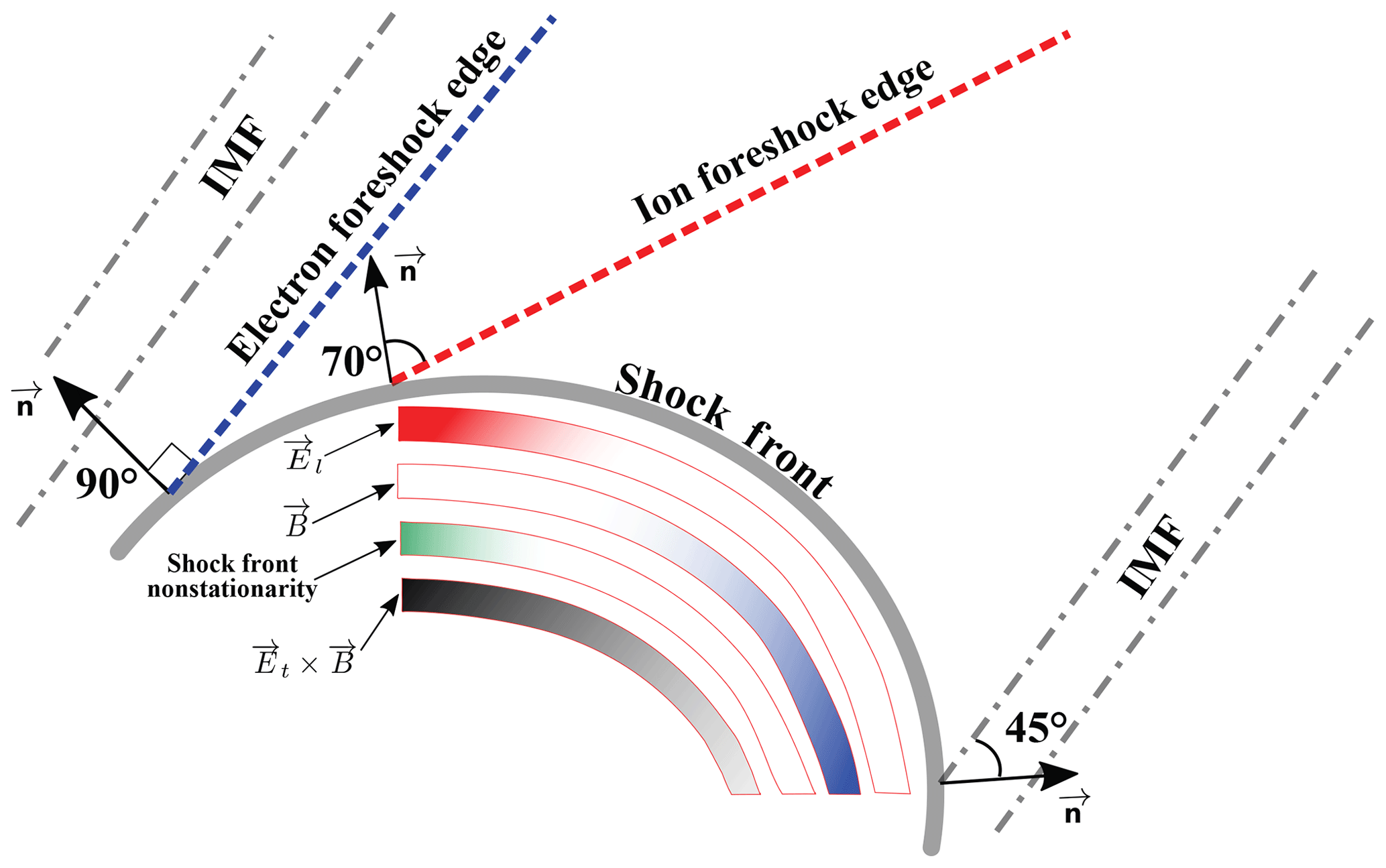
Figure 11 Sketch of the ion foreshock in the quasi-perpendicular shock region, illustrating the angular areas along the curved front where the four main identified processes contributing to and/or impacting on the formation of back-streaming ions apply (namely the longitudinal electric field E_l, the magnetic field, the shock front nonstationary and the convective electric field E_t). Each process is illustrated by different thick band along the curved front which is shifted, one from the other, in order to avoid overwhelming the sketch. One color (red, blue, green and black, respectively) is associated to each process. The varying intensity of the color indicates where the process is strong (full color) or weak (white). This allows one to identify, at a glance, the angular areas where the different processes are complementary or accumulating. The upstream interplanetary magnetic field (IMF) is reported in gray (dotted and dashed lines), as is the shock front itself. Typical directions θ_Bn=90 and 70^∘ (blue and red dashed lines) defined between the local shock normal n and the IMF indicate the location where the electron and ion foreshock edge initiates from the curved shock front, respectively. The electron foreshock edge is indicated as a reference.

6 Conclusions

Present test particle simulations reinforce the scenario described in Savoini and Lembège (2015) and have allowed us to investigate the formation of the ion foreshock more deeply. In summary, the impact of the three quantities or effects has been identified as follows: (i) the electric field (separately the ${\stackrel{\mathrm{̃}}{E}}_{\mathrm{l}}$ and the ${\stackrel{\mathrm{̃}}{E}}_{\mathrm{t}}$ components), (ii) the magnetic field and (iii) the shock front nonstationarity. The synoptic of Fig. 11 summarizes the importance of each impact versus the shock front curvature from the edge of the ion foreshock (${\mathit{\theta }}_{\mathrm{Bn}}\approx \mathrm{70}{}^{\circ }$) to ${\mathit{\theta }}_{\mathrm{Bn}}=\mathrm{45}{}^{\circ }$. In this sketch, the colors vary from strong (full color) to weak (white) intensities as a function of their respective influence on the ion dynamics. These different effects are the following:

1. Impact of the E_l field on the ion reflection process. As is well known, the built-up potential wall at the shock front (i.e., the electric field E_l along the shock normal n) is mainly responsible for the deceleration (i.e., acceleration in our reference frame) of the incoming upstream ions by the shock front. The E_l component has essentially two distinct impacts where, (i) without this electric component, no reflected ions are observed for ${\mathit{\theta }}_{\mathrm{Bn}}>\mathrm{62}{}^{\circ }$, whereas in presence of this electric component reflected ions (having suffered even one bounce) can be observed at the edge of the ion foreshock ($\approx {\mathit{\theta }}_{\mathrm{Bn}}\le \mathrm{70}{}^{\circ }$); (ii) at lower angles (${\mathit{\theta }}_{\mathrm{Bn}}\le \mathrm{50}{}^{\circ }$) many ions are reflected without the help of the ${\stackrel{\mathrm{̃}}{E}}_{\mathrm{l}}$ component and can be associated to a magnetic mirror reflection. Then, in Fig. 11, ${\stackrel{\mathrm{̃}}{E}}_{\mathrm{l}}$ is only reported as being strong around the edge of the ion foreshock to emphasize its mandatory action for high θ_Bn angles.

2. Impact of the E_t field on the ion reflection process. Figure 10 evidences that the convective electric component E_t is always present in our simulation (we are in the solar wind reference frame and then E_t≠0 within the curved propagating shock front). Our previous work (Savoini and Lembège, 2015) was only able to show that the E×B drift scenario in the velocity space foreseen by Gurgiolo et al. (1983) was at the origin of two distinct GPB (i.e., one bounce) and FAB (i.e., multibounces) populations only separated from the particle time history within the shock front.

   But this scenario was not able to distinguish the relative importance between the two electric field components of E_l and E_t, respectively. This question has been clarified in the present paper since FAB and GPB populations formed by the E×B drift in the velocity space are evidenced with or without the E_l component (Fig. 10). Then, the E_l field seems to be less dominant than the E_t field. Finally, Fig. 11 illustrates the E×B drift impact by a dark color that is almost uniform within the whole quasi-perpendicular region.

3. Impact of the B field on the ion reflection process. The magnetic field is important for several reasons: (i) its increase at the shock front builds up the E_l component (space charge effect), which reflects back incoming low-energy ions, and (ii) more importantly, it is also directly responsible for the reflection of some ions (i.e., through the magnetic mirror reflection) and for the drift along the shock front of the multibounce ions (i.e., FAB population). Then, this population gains energy as ions propagate in the E_t direction along the shock front. Nevertheless, as θ_Bn decreases from 90 to 45^∘, the ion reflection becomes easier since the parallel guiding center velocity needed to overcome the shock front velocity decreases (Paschmann et al., 1980). This behavior is clearly illustrated herein by the increase in the percentage of reflected ions BI_% as θ_Bn decreases (i.e., N_Box increases). This behavior persists even in absence of E_l, where BI_% is only reduced by a factor of 2.5, as illustrated by Fig. 6. Then, if the magnetic field is important in the whole quasi-perpendicular region, we emphasize, in Fig. 11, its stronger impact near ${\mathit{\theta }}_{\mathrm{Bn}}\approx \mathrm{45}{}^{\circ }$ where it is mainly responsible for the reflection (i.e., magnetic mirror) and acceleration (i.e., Fermi-type) of ions (Webb et al., 1983).

4. Impact of the shock front nonstationarity. Present simulations show that the reflection process is not continuous in both time and space but strongly depends on the local shock front profile met by incoming ions at their hitting time. This behavior is difficult to identify in experimental measurements since the particles coming from different shock locations and at different times are mixed; in contrast, this can be easily evidenced in our HE test particles configuration. This configuration evidences that particular shock profiles are more suitable for the formation of back-streaming ions than other ones. Indeed, we observe modulations of the BI_% percentages in Fig. 9 which are much more pronounced than in our FCE configuration (Fig. 8). These modulations are so strong that BI_% drops to zero periodically, which means that for certain shock front profiles no ion can escape into the upstream region. This behavior is observed for all N_Box at the same time (i.e., same shock profile), which implies that the ion reflection does not depend on the location along the shock front but essentially on the global profile of the shock at a given time. In the present simulations, we can identify four distinct and noticeable bursts (i.e., maxima BI_% values) with an average cyclic occurrence period of $\mathrm{1}{\stackrel{\mathrm{̃}}{\mathit{\tau }}}_{\mathrm{ci}}^{\mathrm{shock}}$ (where ${\stackrel{\mathrm{̃}}{\mathit{\tau }}}_{\mathrm{ci}}^{\mathrm{shock}}$ is defined at the shock ramp). Surprisingly, N_Box=0 (Fig. 9) does not show the same bursts as the others, which suggests that the time variations in the shock front (and associated particle diffusion, as suggested by Kucharek et al., 2004) are mandatory for obtaining back-streaming ions around the edge of the ion foreshock (i.e., high θ_Bn). This point will require a further investigation.

In summary, present results show that the formation of the ion foreshock is not a continuous process but must be considered as time dependent, which leads to bursty emissions of back-streaming ions. Three different contributions have been evidenced, namely (i) the E_l component in the ion global reflection process, in particular for high θ_Bn, (ii) the magnetic field B essentially observed when E_l=0 for lower θ_Bn, such as the magnetic mirror reflection, and (iii) finally, the E_t×B drift in the velocity space mainly sustained by the convective electric field which is necessary to generate both FAB and GPB populations as described in Savoini and Lembège (2015).

Unfortunately, the impact of the shock front nonstationarity on the ion foreshock is difficult to analyze (see, for example, Fig. 7) for two different reasons, namely (i) the time-of-flight effects mix reflected ions coming from different shock profiles, and (ii) even if some shock profiles are more efficient than others at reflecting ions, their respective impacts disappear rapidly since they are being blurred out by the impact of less efficient profiles on particles as time evolves.