Ducting of incoherent scatter radar waves by field-aligned irregularities

We provide an explanation for a mysterious phenomenon that has been recognized in recent years in European Incoherent Scatter (EISCAT) UHF incoherent scatter radar (ISR) measurements during many high-power high-frequency (HF) ionospheric pumping experiments. The phenomenon is an apparent increase in electron density observed above the HF reflection altitude, extending up to the observable limits usually in the range 400–650 km, as shown in several publications in recent years. It was shown by Senior et al. (2013) that several examples of these enhanced backscatter could not be explained by increases in electron density. A summary of characteristics of the backscatter enhancements is presented as well as the results of a survey of events. We propose that medium- to large-scale HF-induced field-aligned irregularities (tens to hundreds of metres scale) act to refract the radar signals along the magnetic field, thereby acting as a guide so that the free-space r⁻² spreading of the signals no longer applies. The nature of the irregularities and the physical mechanism of their production by powerful HF waves is an exciting topic for future research since, surprisingly, they appear to be preferentially excited by X-mode waves. The explanation proposed here involving HF-induced irregularities may well apply to other ISR observations of the ionosphere in the presence of specific natural irregularities.

1 Introduction

The high-frequency (HF) radar facility (Rietveld et al., 2016) near Tromsø, Norway, consists of 12 transmitters of nominally 100 kW, covering the frequency band from 4 to 8 MHz, which can be connected to one of three antenna arrays. Array 1 covers 5.5–8.0 MHz with a mid-band gain of 30 dBi (decibels isotropic), Array 2 covers 4–5.5 MHz with a mid-band gain of 24 dBi, and Array 3 also covers 5.5–8.0 MHz with a mid-band gain of 24 dBi. In many HF pumping experiments with the European Incoherent Scatter (EISCAT) facilities near Tromsø (69.6^∘ N, 19.2^∘ E) during the recent solar cycle maximum, when ionospheric F-region critical frequencies were commonly in the range 5.5 MHz to more than 8 MHz, apparent increases in electron density were observed by the 933 MHz incoherent scatter radar above the HF reflection height when the radar was pointed along the geomagnetic field. Some of these are shown in published papers by Blagoveshchenskaya et al. (2011a, 2011b, 2013, 2015, 2017, 2018), Cheng et al. (2014), Borisova et al. (2016, 2017), Wu et al. (2017), and Senior et al. (2013), and they have been presented by us in several conferences and workshops. They have been observed rather often, but no systematic study has been made so far. Some characteristics as observed by these authors, which can be seen in several of the published examples listed above, are given here. The enhancements extend from about the HF reflection height to as high an altitude as there is still enough backscatter to be detected, typically 400–500 km. Importantly, they are observed only when the UHF radar is within 0.5^∘ (Bazilchuk, 2019) of the geomagnetic field. They are excited by both ordinary- and extraordinary-mode (O- and X-mode) HF pumping but more commonly with X-mode pumping (see survey below and Blagoveshchenskaya et al., 2018), with an enhancement factor reaching two for X-mode heating (Blagoveshchenskaya et al., 2018; Bazilchuk, 2019). They have usually been observed with HF pump frequencies of 5.4 MHz and above, although there seems to be one published case near 4.9 MHz (Blagoveshchenskaya et al., 2011a), and we have found two cases at 4.544 MHz (see the Supplement). They appear within some tens of seconds after HF turn on, but this is poorly documented and studied. The decay times are similarly poorly studied but seem to be a few tens of seconds to a few minutes. When stepping in frequency around a harmonic of an electron gyrofrequency using an O-mode HF pump wave, the enhancements are strongest when the pump is near or above the gyroharmonic (Blagoveshchenskaya et al., 2018). They appear to be anticorrelated with HF-induced electron temperature increases as shown in Fig. 1 of this paper, Fig. 2 of Borisova et al. (2016), Fig. 3a of Borisova et al. (2017), and Fig. 4 of Blagoveshchenskaya et al. (2018).

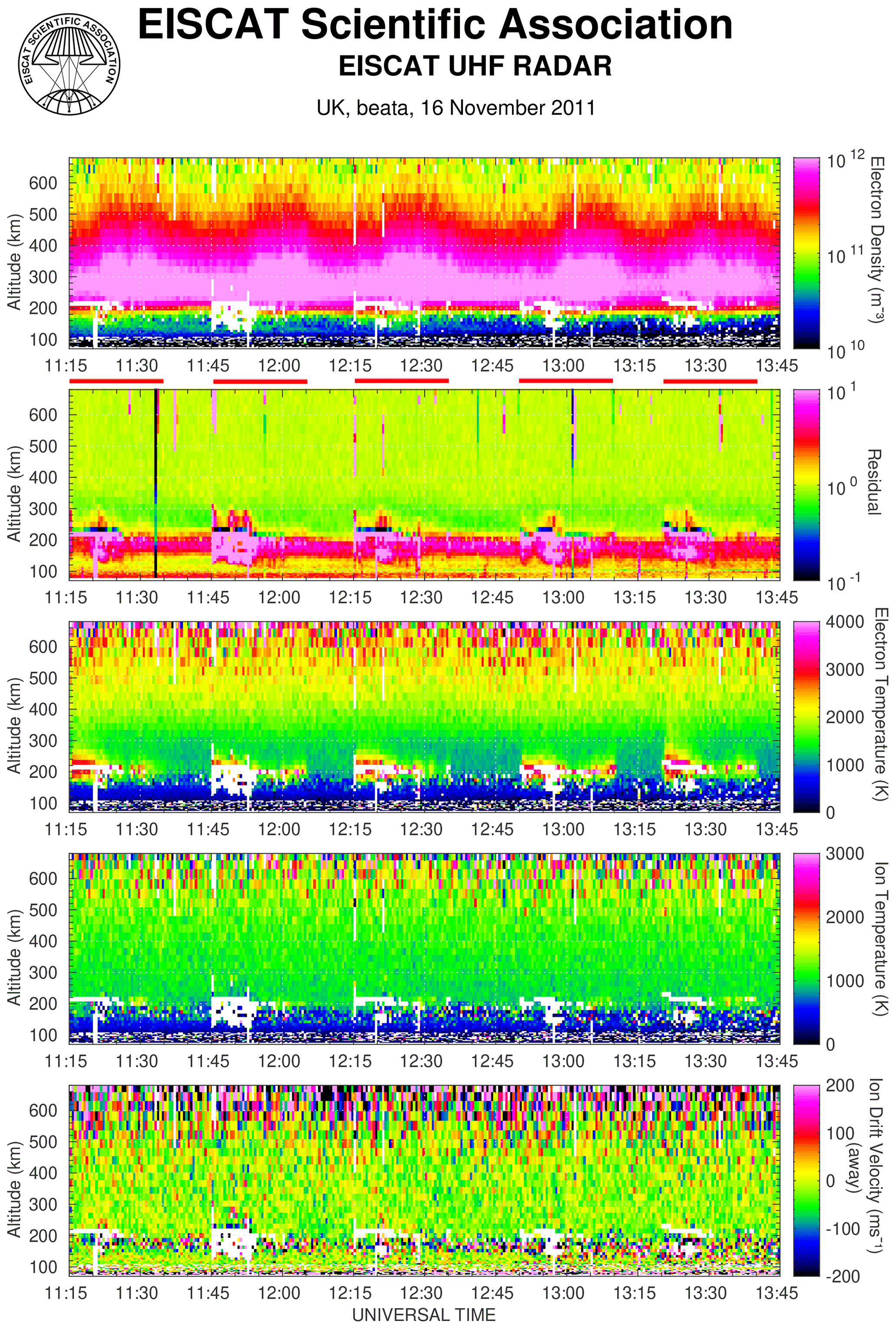
Figure 1 An example of wide altitude ion line enhancement (WAILE). The top panel shows the enhancements interpreted by the analysis as an electron density increase between about 200 and 600 km. The HF on times are shown by red bars above the second panel. The second panel (Residual) shows that the measured spectra agree well with theoretical spectra for a Maxwellian plasma since the residual is near one. The blank areas have residuals over 10 which are regarded as having poor fits.

The apparent density enhancements were interpreted as such because they result from a good theoretical spectral fit to the measured ion line spectra, which were not affected by enhancements caused by plasma instabilities, which occur in a narrow altitude band at and below the HF reflection height. To a first-order approximation, the electron density is proportional to the backscattered power of the ion line. Senior et al. (2013), however, showed a typical example which could not have been a real density enhancement, because the natural plasma frequency at the relevant heights showed no corresponding increase. Furthermore, they showed another case from 2001, near the previous solar cycle maximum, where the apparent density enhancement seen by the Tromsø UHF radar near 300 km was not seen by the two remote receiving antennas in Kiruna and Sodankylä when pointed to that common volume at 300 km. Because the enhancements are in the backscattered ion line, they have been called wide altitude ion line enhancements or WAILEs for short. Subsequent examination of the plasma line backscattered power in the first case studied by Senior et al. (2013) showed that it was also enhanced by approximately the same amount as the ion line power, showing that the effect is caused by some increase in backscattered radar power at UHF frequencies, irrespective of whether the scattering is from ion acoustic or electron acoustic plasma waves. Figure 3 of Borisova et al. (2017) confirms this increase in plasma line power at 300 km for another event associated with the X-mode-induced ion line power enhancements and the apparent electron density increases, well above the reflection height of the HF wave at around 230 km.

We first present an example of the WAILE phenomenon pointing out some of the features. Next the results of a survey to investigate the occurrence frequency of WAILEs and some of their features will be presented. Then we present an explanation of the phenomenon in terms of refraction and guiding of VHF and UHF radio waves by field-aligned elongated electron density irregularities. To support this model, some ray-tracing results are presented. Finally, possible implications for other incoherent scatter radar (ISR) measurements of the natural ionosphere are presented.

1.1 Example of a WAILE

We present an example in Fig. 1 which shows the apparent density enhancements during an experiment on 16 November 2011 where the O-mode HF pump wave was modulated in a 30 min cycle of 20 min on and 10 min off starting at 11:15:05 UT and again at 12:50:05 UT. The HF on times are indicated by red bars above the second panel. The HF beam and the 933 MHz ISR beam were pointed along the magnetic field line, 12^∘ S of zenith, and the HF effective radiated power was calculated to be approximately 660 MW O mode and 11 MW X mode. During the on period, the frequency was first constant at 6.7 MHz for 2 min after which it was stepped up every 10 s to 7 MHz in 108 steps of 2.778 kHz each. The fifth harmonic of the electron gyrofrequency is calculated to be 6.862 MHz at 200 km using the IGRF (International Geomagnetic Reference Field) magnetic field model for 2011. This example, from a standard analysis using 30 s integration time, shows several of the typical features mentioned above, but it is also a complicated example because of the frequency stepping and slightly atypical in that it is for O-mode heating. No attempt was made to remove backscatter from satellites or ion lines enhanced by plasma instabilities near the reflection height of the HF wave. The WAILEs are seen as the periodic apparent electron density increases between 300 and 600 km, in synchronism with the HF. The rise time of the WAILEs are not easy to determine from this experiment, because the initial enhancement after HF turn on is very weak and barely noticeable in this plot until about 7 min after each start, when the frequency has reached about 6.78 MHz. After that the enhancements are very clear until the end of the HF pulse, when they decay in about 2 min. A slight dip in the WAILE is apparent for about a minute in the first, second, and fifth HF pulses at about 8 min before the end of each pulse when the frequency is near the gyroharmonic at 6.86 MHz. This interesting frequency dependence will not be investigated further in this paper, but it is an important aspect for further studies. Gyroharmonic effects are seen in many phenomena resulting from HF pumping, such as irregularity formation (Honary et al., 1999), stimulated electromagnetic emissions (SEEs) (Stubbe et al., 1994; Honary et al., 1995; Leyser et al., 2001), and electron acceleration (Gustavsson et al., 2006).

Figure 2 Ray paths of a set of 40 up-going 933 MHz waves from the transmitter at (0, 0) with launch zenith angles evenly spaced between 0 and 0.3^∘ passing through a region of vertically aligned irregularities, shown in grey shading, with $A=\mathrm{1}\times {\mathrm{10}}^{-\mathrm{6}}$, W=50 m, and L=80 km between 220 and 300 km. The magnetic field lines are assumed to be vertical. These rays illustrate the effects of refraction, but in the final modelling we use 3333 realistically spaced rays both sides of zenith to represent the transmitted beam.

Figure 3 Backscattered down-going 933 MHz rays from one of the up-going rays which arrived at 600 km in Fig. 2. The 51 rays pass through the same region of irregularities as in Fig. 2 with $A=\mathrm{1}\times {\mathrm{10}}^{-\mathrm{6}}$, W=50 m, and L=80 km between 220 and 300 km. The magnetic field lines are assumed to be vertical. There is a clear increase in the density of rays (or backscattered power) near the receiver antenna at (0, 0), as well as regions of weaker backscatter further away. In the modelling it is the number of rays from 3333 sources at 600 km that arrive within the 32 m antenna length at 0 km and within the antenna beamwidth that determines the final backscatter strength.

The second panel, labelled “Residual”, shows a parameter which should be close to one for a good fit of the measured spectrum to a theoretical spectrum for a Maxwellian plasma. It is calculated here as proportional to the difference between the measured and theoretical autocorrelation function divided by the expected (theoretical) variance. It shows that the theoretical spectra were a very good fit at most heights above about 220–300 km. The region between 150 and 200 km shows higher values than one because of the gradient in ionospheric parameters and the ion composition changing, which are not taken into account in the theoretical variance calculation where a homogeneous plasma is assumed. The white areas have residuals greater than 10 and are mostly the results of non-thermal plasma excitation near the HF reflection height (near 200 km) or satellites in the radar beam which were not removed for this analysis. The residuals near one show that the derived electron density, temperature, ion temperature, and velocity are reliable. There is some localized electron heating above 220 km extending up to 300 km and sometimes beyond which is most pronounced in the first 8 min of most of the HF pulses, when the WAILEs are weakest. This illustrates the observation made above that the WAILEs anticorrelate with HF-induced electron temperature increases. This electron heating is a well-known phenomenon associated with upper-hybrid plasma instabilities and the formation of decametre-scale striations when pumping away from a gyroharmonic (Honary et al., 1995). The observation that WAILEs are observed more frequently with X-mode pumping ties in with the anticorrelation with electron temperature enhancements since X-mode pumping results in relatively weak Ohmic heating compared with resonant heating from O-mode pumping (e.g. Bryers et al., 2013). A very similar observation to the example in Fig. 1 is shown in Fig. 6 of Borisova et al. (2016) for the sixth gyroharmonic.

2 Survey of events

To provide some statistical evidence of the conditions under which the WAILE phenomenon is observed, a search was performed of all experiments carried out in the period 1 January 2001 to 6 July 2018 (the date when the search was begun). As anecdotally there is little evidence of WAILEs during experiments using antenna Array 2 (restricted to frequencies below 5.5 MHz) and since Array 3 (frequencies above 5.5 MHz but lower gain than Array 1) was inoperative for part of the period, the search was confined to experiments using Array 1.

The search was performed in two parts. Firstly, an automated process was used to scan the computer-generated experiment log files to identify cases where Array 1 was used and where the pump frequency was below the F-region critical frequency. Then the resulting list of cases was used to manually inspect quick-look plots of the UHF radar data to determine whether or not WAILEs were observed for each case.

The automated process defined a “case” as a UT hour during which (a) at least two transmitters were active on Array 1 and (b) the lowest pump frequency used was below the highest ordinary wave critical frequency, foF2, measured by the EISCAT Dynasonde (Rietveld et al., 2008) during the hour plus a margin of 0.81 MHz. The margin is approximately the value by which the extraordinary wave critical frequency, fxF2, exceeds foF2 and means that experiments where the pump frequency was below the F-region critical frequency would be included regardless of the polarization (O or X mode) used. If no Dynasonde data were available for the hour in question, condition (b) was not applied to avoid unnecessarily excluding useful cases at this stage.

The manual process inspected quick-look plots of the UHF radar data available in the EISCAT data archive together with the manual logs of HF facility operations. For each case, it was first determined if the experiment mode was suitable for observation of WAILEs: the UHF radar must have been pointed in the field-aligned direction for at least part of the hour and running in a mode providing F-region coverage; the HF facility must have used pump-on periods greater than about 30 s. Then for suitable cases, the UHF radar electron density range–time plots were inspected to decide whether WAILEs were observed with either O- or X-mode pumping during that hour.

The result of the search was a list of cases giving the UT date and hour of each case, the minimum pump frequency, and maximum foF2 during that hour as well as a set of codes indicating whether the experiment was unsuitable, quick-look plots were unavailable, or if WAILEs could or could not be convincingly identified for O- and X-mode pumping if each polarization was used. The results of the search are available in the Supplement.

The main shortcoming of this search is the manual identification of the presence of WAILEs, which is necessarily subjective. This, together with the inevitable risk of human error in inspecting the data and recording the results, adds a degree of uncertainty to the results. Fully automating the process was deemed unfeasible. To do so would have required automatically analysing the electron density data to compare the density between pump-on and pump-off periods. The computer-generated log files give the transmitter status only at discrete time points and this would make reconstructing the pump cycle ambiguous.

The search resulted in a total of 1449 cases, of which 606 were useful (experiment mode suitable, quick-look data available) and were used for further analysis.

Table 1 shows the observed occurrences of WAILEs with O- and X-mode pumping. A pooled two-proportion z test comparing the proportion of cases with WAILEs between O and X modes rejects the null hypothesis that the proportion is the same with a z score of 7.7, indicating strong evidence that the proportion is higher with X mode.

Table 1 Counts and proportions of WAILE occurrence for O and X modes.

3 Suggested explanation

We now suggest a mechanism whereby the backscatter enhancements are explained in terms of UHF radio wave propagation along large-scale irregularities, but we make no attempt to explain the more interesting problem of the creation of the postulated irregularities. In standard incoherent scatter radar theory, it is usually assumed that at 933 MHz the radar transmissions propagate in straight lines as in free space, because that frequency is very much larger than the maximum ionospheric plasma frequency which may reach 10–20 MHz at the most in the F region. A radio wave at 933 MHz, however, does experience some weak refraction from refractive index changes caused by electron density irregularities. An electromagnetic wave propagating at a small angle to a plane where the refractive index changes will experience refraction. The ionosphere and magnetosphere is full of electron density irregularities at various scales which are aligned along the magnetic field. At the critical angle, given by sin${}^{-\mathrm{1}}(n_{\mathrm{2}}/n_{\mathrm{1}})$, where n₁ and n₂ are the refractive indices at an interface, a ray will be refracted so as to propagate parallel to the interface, and for larger angles the ray will be totally reflected at the interface if n₂<n₁.

For simplicity, let us assume that the HF pumping creates magnetic-field-aligned irregularities with a 5 % electron density depletion spaced tens of metres apart starting near the HF reflection height of typically 200 km and extending several tens of kilometres along the magnetic field. This depletion is close to the average 6 % depletion found during a rocket measurement of heater-induced irregularities over the Arecibo facilities (Kelley et al., 1995). With a background electron density (N_e) of $\mathrm{8}\times {\mathrm{10}}^{\mathrm{11}}{\mathrm{m}}^{-\mathrm{3}}$ or plasma frequency of 8 MHz, this gives a critical angle for a 933 MHz wave of 89.889^∘, which is a grazing angle of 0.111^∘. This means that all rays within 0.111^∘ of the field-aligned direction will be ducted by the irregularity and will not fall off with the usual r² dependence as rays outside this angle will. The one-way half-power beamwidth of the UHF radar is 0.6^∘ (Folkestad et al., 1983), which is also the value for the “opening angle” used by the GUISDAP incoherent scatter analysis software (Lehtinen and Huuskonen, 1996). For field-aligned pointing, the ducted solid angle is therefore 14 % of the total solid angle of the transmitted beam (solid angle =2π (1−cos(θ)), where θ is half the apex angle of the subtended cone).

For a background plasma frequency of 5.4 MHz with a 5 % density depletion, the grazing angle for critical incidence is 0.074^∘, which corresponds to only 6 % of the solid angle of the transmitted beam, which could largely explain why the ducting effect is smaller and has not been observed very often for heating frequencies less than 5.4 MHz.

The proposed mechanism also explains why backscatter enhancements were never seen at the remote receiving stations when they were still operating at 933 MHz. In the WAILE example from 11 November 2001 presented by Senior et al. (2013), the remote receivers in Kiruna and Sodankylä showed no enhancements, while the backscatter signal received at Tromsø did. This is understandable from our ducting model for two reasons. Firstly, the volume of the scattering region above Tromsø as seen from the remote sites is much larger because of the greater distance to the receiver, so the horizontal redistribution of radar power from Tromsø is mostly contained within the receiver's field of view. Secondly, the scattered signals to the two stations are at such a large angle to the magnetic field (18 and 28^∘ for Kiruna and Sodankylä, respectively, at 278 km above Tromsø) that they are effectively not refracted by the irregularities.

4 Ray-tracing model

To give a more detailed model of the ducting hypothesis, we performed some two-dimensional ray tracing of 933 MHz radio waves in a medium with sinusoidal refractive index irregularities perpendicular to the direction of propagation and a limited spatial extent in the main direction of propagation. The ray-tracing equations were solved initially using the differential equation solver lsode.m in GNU Octave (version 4.4.1) and later using ode45.m in MATLAB in order to speed up the calculations.

The irregularities are modelled by a refractive index $n=\mathrm{1}+f\left(r\right)$, where n is the refractive index at r, the position vector (x, y) of a point on the ray, and f represents irregularities with a sinusoidal variation in the x direction. We assume that the magnetic field is vertical, i.e. along y. In the y direction, the irregularity amplitude is tapered by 1+tanh (y) functions to give gradual transitions into and out of the irregularity region. We use the following formula:

$$\begin{array}{}\text{(1)}& \begin{array}{rl}f\left(r\right)=& A\cdot \mathrm{0.5}\cdot (\mathrm{1}+\tanh (y-y_{\mathrm{0}})/S_{\mathrm{0}})\cdot \mathrm{0.5}\\ \cdot & (\mathrm{1}-\tanh (y-y_{\mathrm{1}})/S_{\mathrm{1}})\cdot \cos (\mathrm{2}\cdot \mathit{\pi }\cdot x/W),\end{array}\end{array}$$

where A is the refractive index perturbation amplitude, y₀ and y₁ are the lower and upper transition points, respectively, of the irregularities; S₀ and S₁ are the lower and upper transition scales, respectively; and W is the irregularity wavelength perpendicular to the magnetic field. The perturbation at the transition points is half that of the maximum, A. In the following example we used a refractive index perturbation amplitude, A, of $\mathrm{1}\times {\mathrm{10}}^{-\mathrm{6}}$ which, for a 933 MHz radio wave, corresponds to 2.7 % change in electron density at $\mathrm{8}\times {\mathrm{10}}^{\mathrm{11}}{\mathrm{m}}^{-\mathrm{3}}$ (8 MHz plasma frequency). The extent of the irregularities, L, in the y direction was 80 km starting at y₀=220 km and ending at y₁=300 km, and they had a wavelength, W, of 50 m in the x direction. The transition scales were fixed with S₀=5 km at the bottom and S₁=20 km at the top of the irregularities. The lower height of 220 km is typically around or just above the reflection height of typical O-mode HF pump waves used in heating experiments, which is where we expect the HF irregularities to be formed. Figure 2 shows the paths of a set of 30 rays uniformly spaced at angles between 0^∘ and 0.3^∘ launched from a point source at the transmitter (0, 0) out to a distance of 600 km along the y axis. Clearly a focusing is seen for rays closely aligned with the y axis with regions of lower ray density further out.

We are simulating a three-dimensional (3D) situation, of which the model is just a slice. In 3D, the density of the rays being proportional to power means that the solid angle subtended by a “bundle” of rays would be inversely proportional to radiated power. So in our 2D model the planar angle between rays is inversely proportional to the square root of the power or simply the wave electric field, E. To approximate the real situation better, we performed such ray tracing with many more rays but with their spacing varying to approximate the narrow transmitted beam of the radar. We used the formula for the radiation field from a circular aperture given by

$$\begin{array}{}\text{(2)}& E=\mathrm{2}\mathit{\lambda }{J}_{\mathrm{1}}\left[\right(\mathit{\pi }D/\mathit{\lambda }\left)\sin \mathit{\theta }\right]/\left(\mathit{\pi }D\sin \mathit{\theta }\right),\end{array}$$

where D is the diameter of the antenna's aperture in metres, λ is the radar wavelength in metres, θ is the angle of propagation from the boresight direction in radians, and J₁ is the first-order Bessel function. The rays were spaced approximately inversely proportional to E.

We next consider the received wave from the scattering region, which is simpler than the transmitted beam, because the incoherent scatter is isotropic. As an example of the scatter from a point along the field-aligned radar beam at 600 km, Fig. 3 shows a set of 51 rays backscattered downwards within a cone of 0.64^∘ along the field line for a refractive index perturbation of $\mathrm{1}\times {\mathrm{10}}^{-\mathrm{6}}$ with a wavelength, W, of 50 m. The radar receiving antenna is at (0, 0) and the perturbations are 220 to 300 km above the radar antenna. One can clearly see a higher density of rays at the antenna caused by the irregularities compared to the uniform distribution of rays one would have without irregularities. There are, off course, also regions where the density of rays is lower, in order to conserve the total energy. If most of the backscattering electrons are within a region of diameter of ∼6 km (the radar beamwidth at 600 km), then some of the ray paths will end up at the antenna with weaker intensity. So the total backscatter seen by the radar is more complicated than these illustrative simplified examples of ray tracing from a single point source. The resultant backscattered signal is the integrated effect of the ducting of the transmitted signal to a large volume and then the many backscattered and partly ducted signals from all the electrons within this relatively large volume.

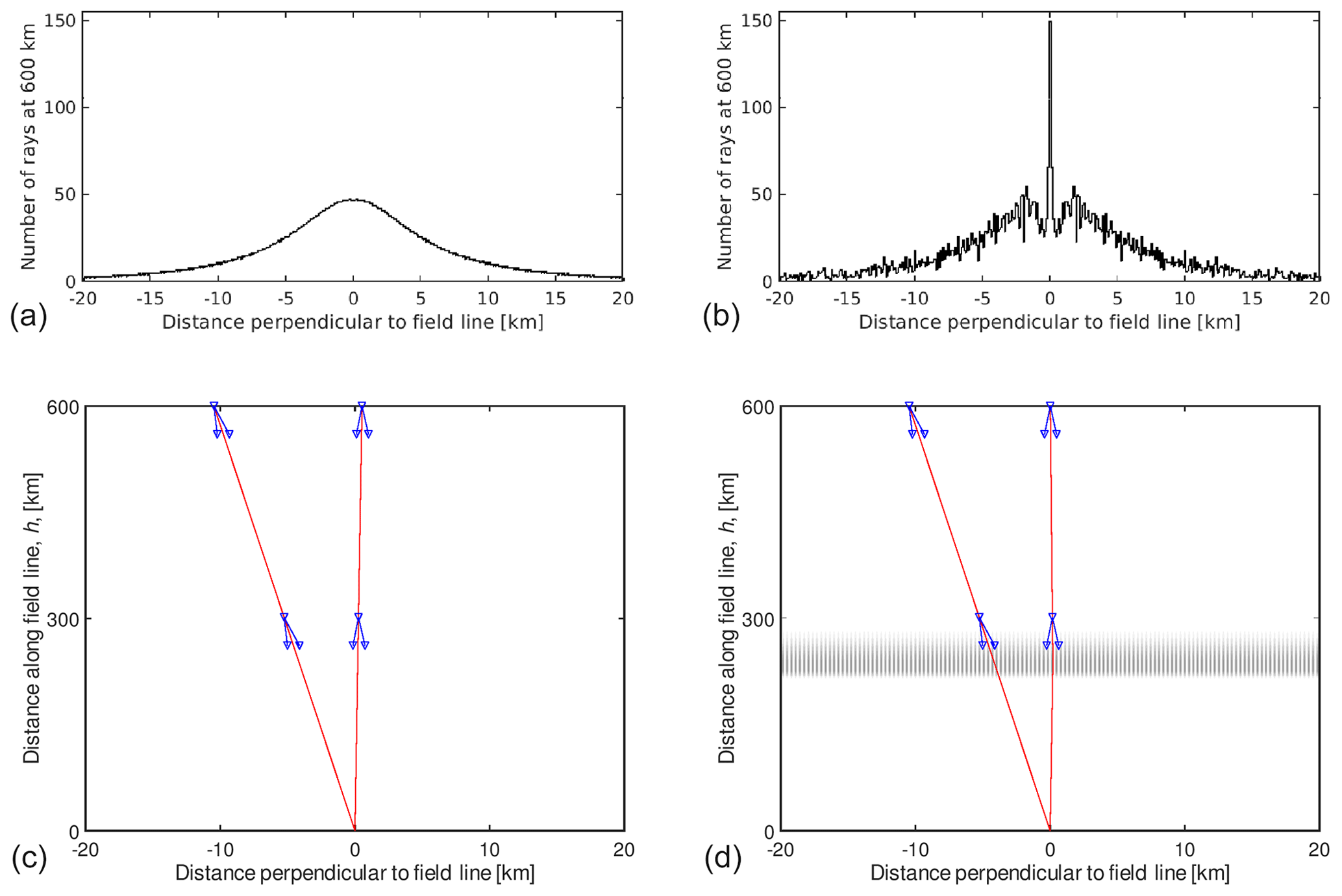
Figure 4 Schematic diagram of the model showing (in red) two out of thousands of rays launched from the transmitter at (0, 0) for the free-space case in (a) and (c) and with field-aligned irregularities (in grey) in (b) and (d). The magnetic field lines are assumed to be vertical. The zenith angles of these two rays are −1 and 0.05^∘. The histograms in (a) and (b) show the distribution of rays arriving at 600 km using a bin width of 100 m. In the modelling, a fan of 30 rays is relaunched from each incoming ray at two heights of 300 and 600 km as depicted by the blue downward arrows which show the edges of the fan at ±0.32^∘ about the incoming ray direction. The histograms in this figure are purely illustrative of one part of the model and are not used in the final modelling. The ratio of the number of rays arriving on the ground within ±16 m of (0,0) and within ±0.35^∘ of the vertical field line for the case with irregularities to the case without irregularities is a measure of the backscatter enhancement measured by the radar.

To make a more realistic model, we used the position of each of the 3333 upward ray's arrival point at height, h, to retransmit a set of 30 rays with launch angles randomly distributed between ±0.32^∘ about the opposite direction with which the up-going ray arrived. These downward-propagating rays meet the same irregularities as the upward rays did. The lower panels of Fig. 4 schematically show two such transmitted rays and the fan of backscattered rays from two heights (300 and 600 km) for the two cases without and with irregularities. Although the backscatter from each point is isotropic, we limit the backscattered rays to this launch cone angle, because we are mainly interested in only those rays that end up within the antenna aperture centred at (0, 0) and within the main beam angle. The number of backscattered rays, n, from each transmitted ray arriving at h is limited to 30 to make the total ray-tracing calculation time acceptable but large enough to give representative and fairly robust results. Tests were made to ensure that the results were not critically sensitive to this number. For example, the ray-tracing results to be presented below were repeated with n=60 and then with launch cone angles of ±0.37^∘ and ±0.27^∘ each using n=30. The average deviation of the enhancement factors for these test cases compared with the model results presented below was less than 10 %.

The intensity of the radar beam is proportional to the number of rays per unit distance in this two-dimensional view, so we can show the density of rays in the form of histograms. The upper part of Fig. 4a shows histograms depicting the distribution of rays arriving at 600 km for the cases without and with irregularities. In free space the distribution is smooth and is determined by the antenna beam pattern as in Eq. (2). The irregularities result in the distribution showing enhancements and depressions. For each ray arriving at height h, 30 rays are launched downwards, randomly distributed within the 0.64^∘ wide fan.

Figure 5 Histograms of the number of rays arriving on the ground from 600 km for (a) when no irregularities are present and (b) after propagating through irregularities having parameters $A=\mathrm{1}\times {\mathrm{10}}^{-\mathrm{6}}$, W=50 m, and L=80 km. The bin width is 32 m, equal to the antenna diameter. There is a clear enhancement in the number of rays arriving at the antenna at 0 km. In the final modelling shown in Figs. 6–9 an extra condition is imposed on the number of rays arriving within the 32 m bin at 0 km, namely that each ray is within the beamwidth of approximately ±0.35^∘.

Figure 5a shows a histogram of the number of rays received at the ground for the case of free-space propagation, i.e. with no irregularities present. As expected, the distribution is uniform, and the edges of the distribution are determined by the limited relaunch cone. The bin width in this histogram and that in Fig. 5b is 0.032 km, equal to the antenna diameter. Figure 5b shows a histogram for the case with irregularities with $A=\mathrm{1}\times {\mathrm{10}}^{-\mathrm{6}}$, W=50 m, and L=80 km. The number of backscattered rays at the 32 m diameter antenna is enhanced in Fig. 5b by about 20 % compared to the smooth ionosphere case in Fig. 5a, but there are also regions of slightly weaker signal within a few kilometres of the antenna. But this is still too simplistic an estimate of the actual enhancement since some of the rays may reach the antenna aperture at incident angles outside the main beam.

For the quantitative results presented below, we count the number of rays arriving within a 0.032 km long segment at the origin, corresponding to the UHF antenna aperture diameter, and with an incident angle of less than ±0.35^∘ to approximate the received signal within the 0.6^∘ half-power beamwidth of the main lobe of the antenna. The ratio of this number to the number of rays received for the case of no irregularities is the measure of the enhanced backscatter strength (enhancement factor) from that height. This ratio was squared to give the enhancement factors plotted in Figs. 6–9 to convert the one-dimensional model results to the two-dimensional reality. The combined effect of these counting conditions (antenna aperture and beamwidth at the antenna) reduces the enhancements considerably compared to the impression one may get from the sketches and histograms in Figs. 2–5.

The results of the ray tracing are presented in Fig. 6 for backscatter from heights of 300 km and in Fig. 7 from 600 km as plots of enhancement factor for four different values of A, the irregularity strength, and 21 different values of the irregularity wavelength, W. Each point in Figs. 6–9 is the result of 999 990 rays being launched from the backscattered height, h, which took approximately 92 min to calculate using MATLAB on a Linux workstation. The smallest irregularity wavelength modelled here is 20 m, equal to 62 times the radar wavelength of 0.32 m, which means that the ray-tracing approach is still valid.

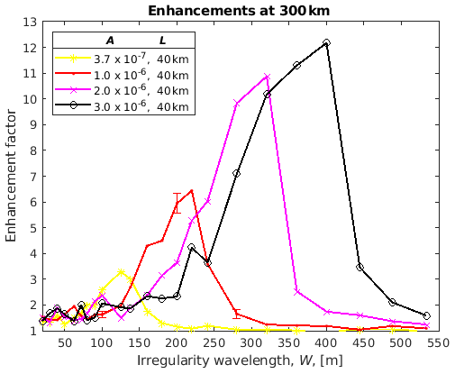
Figure 6 Enhancement factors for 933 MHz backscatter from 300 km calculated from the density of rays entering the antenna beam compared to the case of free-space propagation for various depths of irregularity, A, and wavelength, W, for a fixed irregularity length, L.

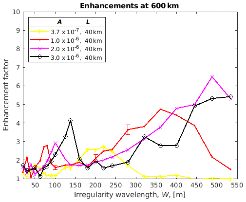
Figure 7 Enhancement factors for 933 MHz backscatter from 600 km calculated from the density of rays entering the antenna beam compared to the case of free-space propagation for various depths of irregularity, A, and wavelength, W, for a fixed irregularity length, L.

The results for the enhancements at 300 km show a systematic variation with irregularity wavelength with stronger enhancements peaking at larger-scale irregularities and the peak being stronger for stronger irregularities. We have never observed such large enhancements as in these peaks with the strongest results being perhaps two. For most of the irregularity strengths with a wavelength less than about 150 m, we find enhancement factors greater than one and less than two. For a given irregularity scale size, one cannot simply conclude that stronger irregularities give stronger enhancements.

To better show the significance of the modelled points, we show three points with error bars in Figs. 6–9 for the case of $A=\mathrm{1}\times {\mathrm{10}}^{-\mathrm{6}}$ and L=40 km. These error bars are the spread in the results after repeating the ray tracing six times. Since the 30 backscattered rays are launched with a random spacing between ±0.32^∘ there will be a different spread in the rays arriving at the antenna on each recalculation. These error bars can be regarded as representative for all the modelled points having similar enhancement factors.

The results for the enhancements at 600 km show a more complex variation which is not so easy to understand. It would appear that the main peak enhancements seen at 300 km get weaker and move to much longer (about 2 times longer) wavelengths, but other peaks appear or get stronger below about 150 m. At 600 km there are enhancements greater than one and less than two for all irregularity strengths over a wide range of wavelengths less than about 280 m.

Figure 8 Enhancement factors for 933 MHz backscatter from 600 km for two lengths of the irregularity, L, along the field line for a fixed irregularity depth, A.

Figures 8 and 9 show the effect on the enhancements at 300 and 600 km, respectively, of having longer irregularities along the magnetic field for the case of $A=\mathrm{1}\times {\mathrm{10}}^{-\mathrm{6}}$. In both cases the curve for 40 km long irregularities is moved to larger irregularity wavelengths when they are 80 km long. For many irregularity scales, the enhancements are larger for the longer-scale irregularities (Figs. 7 and 8). The peak enhancements in Fig. 6 and largely in Fig. 7 are greater as irregularity strength, A, is increased. Both these effects might be expected since stronger and longer irregularities should help guide the rays.

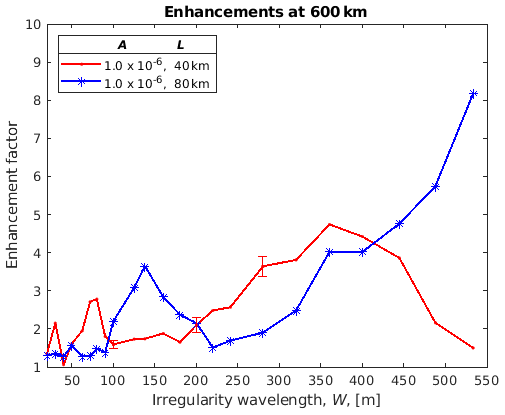
Figure 9 Enhancement factors for 933 MHz backscatter from 600 km for two lengths of the irregularity, L, along the field line for a fixed irregularity depth, A.

For the 12 October 2012 event studied by Senior et al. (2013), the enhancement factor was fairly constant with altitude with the value ∼1.5. If we were to take an amplitude of 10⁻⁶ and 40 km length, then the red curve in Figs. 6–9 would suggest a transverse scale between about 90 and 130 or ∼50 m in order to get a similar enhancement at 300 and 600 km. We have no independent data to check this prediction, but the numbers do not seem unreasonable. For other irregularity strengths or lengths, we would get different transverse scales.

We note that the smallest scale of irregularities we have modelled here (W=20 m) is close to the decametre scale of irregularities that produce backscatter on HF radars like SuperDARN (Super Dual Auroral Radar Network). There does not seem to be an obvious connection between CUTLASS (Co-operative UK twin-located Auroral Sounding System) radar backscatter and WAILEs, although this should be studied more closely. HF pumping produces decametre-scale irregularities that are often correlated with electron temperature increases so this would suggest that they might anticorrelate with WAILEs.

The ray-tracing modelling results suggest that WAILEs should be quite sensitive to the spectrum of irregularities produced by HF pumping and might thereby become a new diagnostic for these irregularities. We should warn, however, against taking the results of the ray tracing here too literally. The model is rather idealized in that it incorporates only one irregularity scale at a time, and in reality we certainly have a large spectrum of irregularities. The modelling here is only intended as a proof of the principle that ducting of the ISR waves can explain the backscatter enhancements. More detailed, independent modelling should be performed to verify our ideas.

5 Evidence of the irregularities

Experimental evidence for large-scale (hundreds of metres to the kilometre scale) irregularities is lacking for most of the heating experiments we have examined at EISCAT. The EISCAT UHF radar cannot directly detect irregularities with scale sizes smaller than the beamwidth, which is ca. 2.4 km at F-region heights. There is evidence for large-scale irregularities from earlier dedicated campaigns, e.g. using radio star scintillations (Frey et al., 1984), but these lacked simultaneous, suitable field-aligned UHF radar data. Honary et al. (1993) deduced the existence of electron density and temperature irregularities along the field with horizontal scale sizes of 6–10 km. We also point out that Kelley et al. (1995) found a wide range of irregularity scales from a rocket experiment through the heated region near Arecibo. They found depletions or filaments with a mean width at half maximum of 7 m with a mean depletion depth of 6 %. The mean spacing between filaments was 15 m, but there was evidence of irregularities at longer wavelengths which they interpret as spacing between bunches of filaments. There is plenty of evidence for decametre-scale irregularities seen by HF coherent radars like CUTLASS (e.g. Senior et al., 2004) but there does not seem to be a correlation between the presence of this backscatter and WAILEs. The presence of such decametre-scale irregularities does not seem to be sufficient to produce WAILEs.

The width of the natural plasma line depends to a large extent on the range of electron densities found within the scattering volume, so this could give an indication of the presence of irregularities, from large to small scales, with the largest scale being limited by the width of the radar beam. There is a suggestion that the natural plasma line measured during the WAILEs studied by Senior et al. (2013) was broadened (unpublished work by one of the authors, AS), but this is something to be examined in future work.

Frolov et al. (2016) show evidence, from the DEMETER satellite, of field-aligned large-scale irregularities (kilometre scale) extending from about 230 km to well over 400 km in height, which act as ducts for very low frequency (VLF) waves. The ducts had dimensions of 80–100 km at heights around 660 km and were produced exclusively by O-mode heating. In many cases, smaller structuring of ∼10 km was seen within the main duct. Such large-scale plasma structuring may well be related to the phenomena we observe. At EISCAT there have been fewer heating experiments performed with DEMETER or similar satellites, and they were sometimes made without ISR observations; thus, we cannot claim to have seen similar irregularities at Tromsø.

6 Predictions for other radars

The refractive index irregularity strength of 10⁻⁶ used in the above examples for a 931 MHz radar wave corresponded to an electron density irregularity of 2.68 % for $N_{\mathrm{e}}=\mathrm{8}\times {\mathrm{10}}^{\mathrm{11}}{\mathrm{m}}^{-\mathrm{3}}$ or an 8 MHz plasma frequency. For the EISCAT 224 MHz VHF radar that is co-located with the UHF radar, this would correspond to a 0.155 % density irregularity so that for a given irregularity strength the focusing effect would be stronger at VHF than at the UHF frequency, neglecting other differences such as antenna beamwidths. So for the commonly used ISR frequency of around 430–450 MHz such as used in the American radars and for the EISCAT Svalbard Radar at 500 MHz the effect would also be larger than at 931 MHz. The high-latitude phased-array radars PFISR (Poker Flat Incoherent Scatter Radar) and RISR (Resolute Bay Incoherent Scatter Radar) can point in the field-aligned direction but not all radars can. The Arecibo 430 MHz and the Jicamarca 50 MHz radars cannot point in the field-aligned direction, and the EISCAT VHF antenna, while physically able to point along the field, is restricted from doing so for operational reasons. So this effect should be stronger for lower-frequency radars, especially in the 220–250 MHz range like the EISCAT VHF radar and the new EISCAT-3D radar (McCrea et al., 2015) being built. Of the radars mentioned here only Arecibo has a HF facility that could produce these irregularities. Unfortunately, the geographical separation of the new EISCAT-3D radar transmitter being built at Skibotn from the present heating facility and the very stringent field-aligned nature of the phenomenon is likely to prevent the WAILE phenomenon being observed directly by the new radar in monostatic mode or with the presently planned bi-static receiver sites. The HF facility cannot tilt its beam in the east–west plane towards the field line at Skibotn. The multi-beam and higher temporal and spatial resolutions expected with this new radar should, however, allow the postulated irregularities to be observed from the side. There are two other lower-frequency ISRs at around 158 MHz: one in Kharkiv, Ukraine, and one in Irkutsk, Russia. Only the Irkutsk radar can point near the field-aligned direction.

7 Implications of the ducting hypothesis

The presence of ducting irregularities described here should also affect signals from radio stars or satellite beacon signals received on the ground. The problem with testing this at the high latitude of Tromsø is that there are few if any signal sources in the field-aligned direction. An increase in scintillation of beacon signals in the field-aligned direction has been seen in very early studies at middle latitudes, e.g. Fig. 1 of Singleton and Lynch (1962). These authors also discuss the same mechanism proposed here, i.e. that of reflection at angles larger than the grazing angle, to explain some scintillation effects. Rush and Colin (1958) show some ray-tracing examples of the effect of long (with respect to a wavelength) cylindrical columns of electrons on various VHF/UHF waves. These papers are concerned mainly with the scintillation phenomena and do not explicitly predict intensity enhancements. Although we have concentrated on the backscatter intensity enhancements, enhanced scintillation of ISR signals may also have occurred. Such scintillation of the received signal is probably masked by the typical integration times of 30 or 60 s used in the incoherent scatter analysis but would be another interesting thing to investigate.

Do natural irregularities, known to occur often in the auroral zone, affect ISR returns in the same way as the HF-induced irregularities? It remains to be seen whether there is something special about the HF-induced irregularities that might make this phenomenon unique to HF pumping experiments. A naturally occurring counterpart might well go unnoticed since electron density will often show variable enhancements due to varying soft or energetic particle precipitation. This same particle precipitation may also produce irregularities which duct the ISR waves, contributing to distortions of the measured density profiles. We emphasize the importance of using plasma line measurements when available with ISRs for determining electron density rather than relying on the ion line due to the possible invalidation of the assumptions concerning the interpretation of the backscatter power, as shown in this paper.

Total electron content (TEC) measurements derived from field-aligned GNSS (Global Navigation Satellite System) differential phase measurements should be examined to see whether irregularities could produce errors in the derived densities, since such waves will also be affected by field-aligned irregularities to a greater or lesser extent depending on frequency.

The fact that X-mode pumping preferentially produces WAILEs over O-mode pumping is an important addition to the variety of other phenomena that have been found in recent years to be excited by X-mode waves and which were expected to be impossible (Blagoveshchenskaya et al., 2017, 2018). The interesting question is how do X-mode waves create the irregularities? We postulate that these irregularities produce the WAILEs. One possibility is through self-focusing of the HF wave, but why this should be more efficient for X mode than O mode is a mystery since the O mode generally produces stronger electron temperature enhancements through upper-hybrid resonance instabilities and thereby stronger irregularities for the self-focusing. These and other questions relating to the effects of X-mode pumping are questions at the forefront of HF active experiments in the future.

8 Conclusions

We have provided a qualitative explanation for the mysterious phenomenon of apparent electron density enhancements seen in magnetic-field-aligned UHF radar data during many HF pumping experiments. The mechanism is refraction leading to ducting of the incoherent scatter radar waves by large-scale density irregularities. This mechanism explains why the enhancements were not observed in bi-static measurements. A simple ray-tracing model explains ISR backscatter enhancements greater than one for a wide range of irregularity scale sizes. The more interesting problem lies in the unknown nature of the irregularities and their excitation by both O- and, preferentially, X-mode pump waves. The postulated irregularities causing the WAILE phenomenon and other effects of X-mode pumping are poorly understood and are at the forefront of HF active experimental research (both experimentally and theoretically). Another intriguing question is whether natural irregularities can produce the same enhancements. Because of this uncertainty, plasma line measurements should be used whenever possible for determining the electron density in ISR measurements when measuring close to or along the magnetic field of the ionosphere. The width of the natural plasma line is another parameter which should be exploited to determine the scale of ionospheric irregularities.