the Creative Commons Attribution 4.0 License.
the Creative Commons Attribution 4.0 License.
 | 24 Sep 2020
Entangled dynamos and Joule heating in the Earth's ionosphere
The Earth's neutral atmosphere is the driver of the well-known solar quiet (Sq) and other magnetic variations observed for more than 100 years. Yet the understanding of how the neutral wind can accomplish a dynamo effect has been incomplete. A new viable model is presented where a dynamo effect is obtained only in the case of winds perpendicular to the magnetic field B that do not map along B. Winds where u×B is constant have no effect. We identify Sq as being driven by wind differences at magnetically conjugate points and not by a neutral wind per se. The view of two different but entangled dynamos is favoured, with some conceptual analogy to quantum mechanical states. Because of the large preponderance of the neutral gas mass over the ionized component in the Earth's ionosphere, the dominant effect of the plasma adjusting to the winds is Joule heating. The amount of global Joule heating power from Sq is estimated, with uncertainties, to be much lower than Joule heating from ionosphere–magnetosphere coupling at high latitudes in periods of strong geomagnetic activity. However, on average both contributions could be relatively comparable. The global contribution of heating by ionizing solar radiation in the same height range should be 2–3 orders of magnitude larger.
- Article
(1146 KB) - Full-text XML
-
Supplement
(172 KB) - BibTeX
- EndNote


The interaction between the ionospheric plasma and neutral wind in the Earth's atmosphere has been described in scholarly textbooks (e.g. Kelley, 2009) and numerous research articles. Still, for a long time the author has felt that his understanding of the subject is incomplete. In this work we describe progress that has been finally made when thinking about the solar quiet (Sq) magnetic variations at mid latitudes. A praiseworthy review of Sq has been published recently by Yamazaki and Maute (2017). Sq is driven by a neutral dynamo. Vasyliūnas (2012) has summarized the fundamental equations for a neutral dynamo and his critical view of the understanding within the community. The conceptual difficulty of the author's interpretation of the neutral dynamo can be phrased less mathematically as follows: in the frame of the neutral gas the product , j the electric current, and E∗ the electric field is in the steady state zero or positive, because of the well-known Ohm's law for the ionosphere. This indicates that Joule heating takes place (which, however, has not been addressed yet in works specifically on Sq, as far as we are aware of). A common comprehension seems to be that the dynamo effect occurs in the Earth-fixed frame where , u the neutral wind, can be negative as required for a dynamo. However, a clear justification for choosing this Earth-fixed frame over any other of the infinitely many possible frames, for example, Sun-fixed or star-fixed inertial frames, seems to be lacking. Undoubtedly Sq variations have to do with neutral motion, but a neutral wind u and associated motional field u×B are frame dependent. In the frame of the neutral gas both are zero. So what exactly drives the Sq currents and fields?
We will first present a new viable steady-state model of the neutral dynamo in the Earth's ionosphere. As the title suggests, it actually involves (at least) two dynamos. A discussion of various aspects of the new model follows, with further references to other works on the subject.
A scenario is considered where the lower thermosphere within two circles of latitude in each hemisphere is connected by the dipolar geomagnetic field, as sketched in Fig. 1. In the Northern Hemisphere branch an easterly (westerly) zonal wind flows, with a westerly (easterly) wind in the Southern Hemisphere. A zero tilt between geodetic directions (westerly, easterly) and magnetic field-aligned Cartesian coordinates is assumed. An ionosphere with a dynamo region exists, as well as magnetized plasma in a plasmasphere (not sketched in Fig. 1). The plasma adjusts to the conditions imposed by the neutral winds but does not interfere otherwise, meaning that neither plasma pressure gradients nor electric fields penetrating from outside, etc., play any role. Zero meridional wind is assumed, and the deviation of the magnetic field B from a vertical inclination in the latitude range of the zonal wind is ignored. The latitude range is small, such that gradients of u, B, and the height-integrated Pedersen conductivity ΣP across the range are neglected. In other words, u, B, and ΣP are assumed constant across the latitudes of the zonal jets. u and B are also assumed constant over the altitude range where there is significant collisional interaction with the plasma. In other words, the ionosphere is assumed to be thin. The scenario is highly simplified compared to any realistic one, in order to achieve a good physical understanding of the situation.

Figure 13-D sketch of a scenario where regions between L=2.5 and 3 are magnetically connected by a dipole magnetic field. The Supplement includes this figure in html format which, when opened in a browser supporting JavaScript, allows one to change the camera view point.
We strive only for a steady-state description. The neutral wind in the Earth's ionosphere at mid latitudes changes only slowly over timescales of several hours, and the plasma between hemispheres would be able to adjust within seconds, practically instantaneously, with only small amplitudes in the transients. We use the jargon and paradigms of the ionosphere community. Astrophysical dynamos (usually without a neutral gas) are typically rather described in terms of a mechanical magnetohydrodynamics (MHD) approach. Differences between the two approaches have been discussed by Parker (1996) for the high latitudes and by Vasyliūnas (2012) for specifically the Earth's neutral wind dynamo. Both authors acknowledged that for the steady state both approaches give equivalent results and that for highly symmetric cases, such as this one, the “traditional” ionospheric E and j paradigm is efficient and mathematically simpler. The electrodynamics of the ionosphere particularly in the steady state and with a neutral gas is treated in a scholarly manner by Kelley (2009).
For completeness we rephrase the most important points relevant for this work: in the reference frame of the neutral gas in the dynamo region, roughly at altitudes 90–200 km, where collisions are significant, an electric field E∗ drives Pedersen and Hall currents JP and JH according to Ohm's law for the ionosphere:
ΣP and ΣH are the Pedersen and Hall conductances and B the magnetic field. The electric field E in other reference frames with the neutral gas velocity u≠0 is
Please note that in many publications this equation is written with the term on the E side, which is the standard form of the Lorentz transformation for non-relativistic velocities u. Often E is measured in some frame (for example the Earth-fixed one), and the task is to estimate E∗. In this work we prefer to write the relation as in Eq. (2). It is here important to note that E∗ is a frame-independent field driving currents according to Eq. (1). The frame-dependent motional u×B does not drive any currents; it is not a real field.
In the topside ionosphere and plasmasphere collisions are rare and the plasma drifts such that , and v is the ion or electron drift. This means that the electric field in the frame of the plasma is zero. The conductivity along B is very high compared to the Pedersen and Hall conductivities, and in the steady state . For constant B, E(z) is also constant (where z is the coordinate along B). This justifies using height-integrated quantities in Eq. (1). When comparing electric fields between the magnetosphere and ionosphere, B is not constant and E is said to “map” between positions along z (Kelley, 2009, Chapter 2.4). For the scenario in Fig. 1 we also require such mapping of E between hemispheres. Owing to the highly symmetric preconditions the mapping is simply that a northward E in the Northern Hemisphere maps to southward in the Southern Hemisphere with equal magnitudes and analogously for reversed directions of E.
The Pedersen current driven by E∗ is associated with Joule or frictional heating (Vasyliūnas and Song, 2005) with power in W m−2:
The divergent JP connects to field-aligned currents (FACs). These currents are associated with a magnetic perturbation in the topside ionosphere (Sugiura, 1984). The difference of the Poynting flux above and below the dynamo region is , matching QJ in Eq. (3) (Richmond, 2010). For the sake of brevity we say that the Poynting flux is downward and equal to the Joule heating rate, for E in the frame of neutral gas, where .
Our aim is to figure out the correct electric field configuration for the scenario sketched in Fig. 1. For this a collapsed 2-D view of the 3-D one, with the northern stripe of zonal neutral wind just above the southern one, is useful. Both regions are viewed from above the dynamo region, respectively. The view is shown in Figs. 2–4. In a first attempt we consider the reference frame fixed to the Earth and assume that . There are still electric fields as a result of the neutral winds in both hemispheres according to Eq. (2), . This first try is sketched in Fig. 2. In both the northern part N and the southern one S, E points southward because both u and B change to opposite directions. But this configuration of E implies a potential drop along magnetic field lines connecting either latitude circles “1” or latitude circles “2” or along both these field lines. Electrons would short circuit such potential drops. Instead, the plasma will establish an electric field E∗ (perpendicular to B) such that potentials along B are avoided. The non-zero E∗ implies that the plasma in the plasmasphere drifts and that there is a velocity difference between plasma and neutral gas. We reject the initial idea that the only electric fields are those of Galilean coordinate transformations from neutral to observer frames.
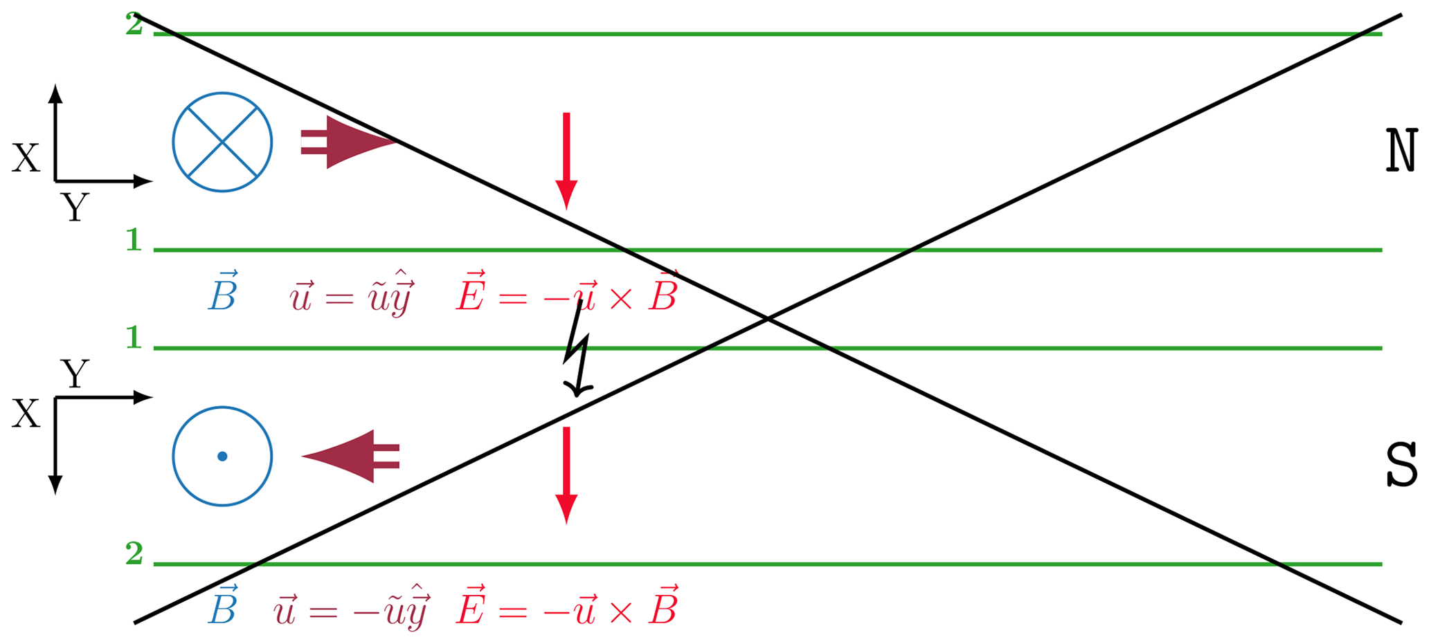
Figure 2Collapsed 2-D view of the scenario sketched in Fig. 1 with the northern and southern regions nearly adjacent to each other and as seen from above the ionospheric dynamo region. The latitude circles labelled “1” and “2” are magnetically connected, respectively. The lightning bolt symbolizes an electrical short circuit along B by electrons that would occur for the suggested E. The large black cross indicates that this scenario is rejected as a possible electric field configuration; please see the text.

Figure 32-D view like in Fig. 2 but in the reference of the northern neutral gas. Electric fields and avoiding potential drops along B are now added, obtaining consistent electric current J, J×B force, magnetic stress ΔB, and Poynting flux .
Now we attempt to find a consistent configuration such that , i.e. a non-zero electric field in the neutral frame. Figure 3 shows the result in the same format as Fig. 2 but in a reference frame where the northern neutral wind is zero, and consequently the easterly wind in the Southern Hemisphere is twice as strong (both N and S are always shown in the same reference frame). Guided by the highly symmetric preconditions we guess that has to point northward with magnitude , with the strength of the wind being . Equations by which E∗ can be determined instead of guessed are given in the following section.
drives a northward current JN, resulting in a westward JN×B force. JN connects to FACs at the edges of the neutral wind jet, where we assume that u and therewith E∗ drop to zero. The magnetic stress ΔB from the current is eastward, from which we derive a downward Poynting flux matching the Joule heating in the N dynamo.
In S is also northward; i.e. and do not map to each other along the magnetic field. Being still in the frame of the northern neutral gas, the southward electric field from the westerly neutral wind is added and gives the total E in S. This field does map to at the conjugate point; i.e. magnetic field lines are equi-potentials. The current JS is driven by the electric field in a zero neutral wind reference frame, which is, for S, . JS correctly closes the current loop between N and S, such that . , which suggests that S is a “dynamo”. This and an upward Poynting flux is consistent with the notion that the S dynamo drives Joule heating in N via Poynting flux from S to N.
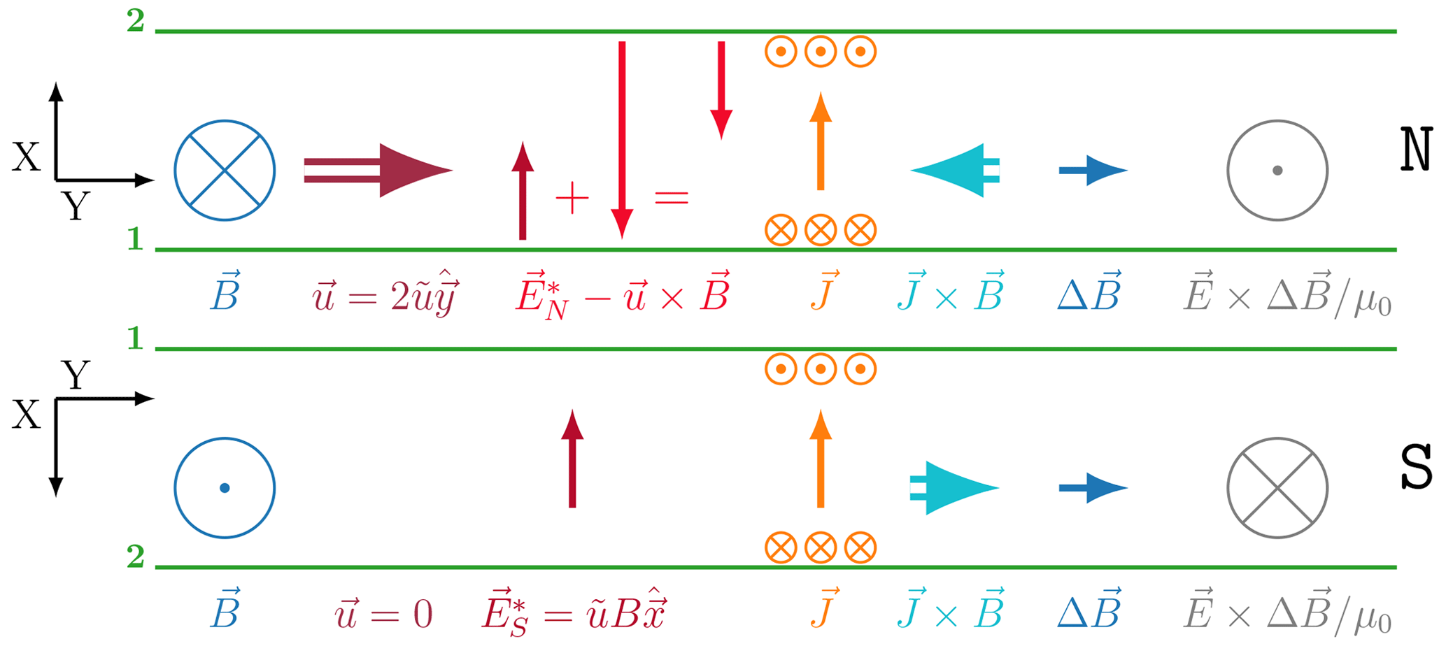
Figure 42-D view like in Fig. 3 but in the reference of the southern neutral gas. Electric fields and that are set up by the plasma to avoid are the same, but the u×B field as a result of the Galilean transformation from the neutral wind frame to the observer is now in the Northern Hemisphere. Please see the text for further discussions.
To fully assert consistency, Fig. 4 shows the 2-D scene in the reference frame where the southern neutral wind is zero. Currents, forces, and magnetic stress are invariant under Galilean transformation and do not change. The total electric field and the Poynting flux are not invariant and so change compared to Fig. 3. It becomes clear that Joule heating also occurs in S, driven by the dynamo in N via Poynting flux from N to S. The magnitude in both hemispheres is the same because of the assumed symmetric preconditions.
The title of this section, “Symmetric dynamos”, does not refer to the zonal winds that are symmetrically opposing in an Earth-fixed frame as drawn in Fig. 1. The same results are obtained for any wind difference that is equal to this symmetric case. “Symmetric” rather refers to equal ionospheric conditions at the conjugate points, equal magnetic field strengths, and perfectly opposing field directions, which is partially relaxed in the following section.
The strengths of currents and forces and the magnitudes of Joule heating and Poynting fluxes are proportional to the Pedersen conductance ΣP. To edge the model a little bit towards a more realistic one, we allow now for different values ΣN and ΣS in each hemisphere. An obvious motivation is that near solstices one dynamo might be sunlit, while the conjugate one is not. In addition, considering the asymmetric case provides an opportunity to write down equations for the fields and instead of guessing them. Requirements that apply for both the symmetric and asymmetric cases include
-
the total electric fields in N and S using the same reference frame need to map onto each other (avoiding a non-zero E∥). We choose arbitrarily the frame of the northern neutral gas (Fig. 3)
for a given zonal wind difference . Δu is positive for .
-
The current loop between N and S closes exactly. In each N and S the current is determined by the electric fields in the reference frame of zero neutral wind, which are and , respectively. The frames of the total E in N and S are not the same. and have opposite north–south directions (for purely zonal winds) because of the orientation of the X axis in each hemisphere, and the field components and have opposite signs:
The solutions of Eqs. (4) and (6) are
and
The Pedersen current is the same in both hemispheres:
Figure 5 shows how E∗ gets adjusted in a situation where ΣN=0.5 S (or mho) and ΣS=1.0 S. The values are perhaps realistically a bit low and could be more different. They were chosen so that the lengths of vectors E in V m−1 and J in A m−1 have the same scale in the figures, for better visual understanding. The reference frame is that of the northern neutral gas. The lower ΣN implies a larger compared to the values in S and also implies stronger Joule heating, which is supplied by a higher Poynting flux from S to N. Please compare with Fig. 6 showing the same scenario but in the frame of the southern neutral gas.
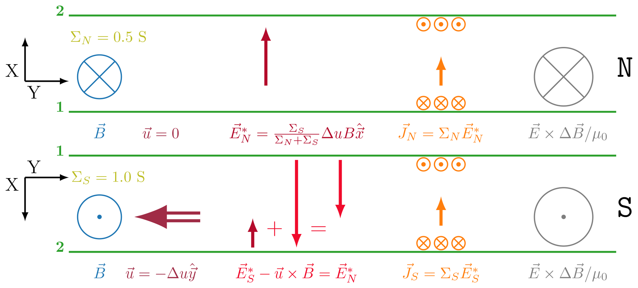
Figure 52-D view in the reference frame of the northern neutral gas like in Fig. 3, but for different conductances in N and S. The electric fields are such that for asymmetric conductances ΣN=0.5 and ΣS=1.0 the same current J is obtained. J×B force and magnetic stress ΔB are omitted in this figure. The sizes of the symbols for Poynting flux in Fig. 6 and this figure are according to the flux magnitudes with the same scale.
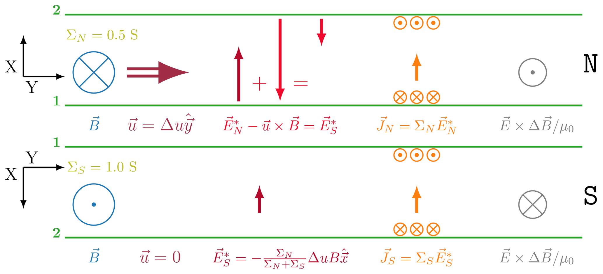
Figure 62-D view in the reference frame of the southern neutral gas like in Fig. 4, but for different conductances in N and S. The electric fields are such that for asymmetric conductances ΣN=0.5 and ΣS=1.0 the same current J is obtained. J×B force and magnetic stress ΔB are omitted in this figure. The sizes of the symbols for Poynting flux in Fig. 5 and this figure are according to the flux magnitudes with the same scale.
The Joule heating in each hemisphere is
and
and the total Joule heating
A low ΣP in either N or S reduces both the current and the total Joule heating.
Asymmetry can also be in the magnetic field, with different field strengths in both hemispheres, BN≠BS. Rather than the simple difference Δu, then winds at conjugate points do not map if
is not zero, and Δw replaces ΔuB in Eqs. (4)–(12). A magnetic asymmetry between hemispheres changes the mapping condition, but it does not cause asymmetry of E∗ or Joule heating.
5.1 The model of entangled dynamos
A current system connecting both hemispheres was suggested first by van Sabben (1966) for Sq. Evidence of interhemispheric field-aligned currents was presented first by Olsen (1997) with Magsat. Paraphrasing Yamazaki and Maute (2017), similar analysis was later performed with the Oerstedt, Champ, and Swarm satellite data; see references therein. Fukushima (1979) had suggested that there are electric potential differences between conjugate points of only a few Volts.
Here we have started by figuring out the electric field configuration for magnetically connected regions in different hemispheres, using a highly symmetric configuration with zonal winds only. Noting that field-aligned potentials would be the result if the condition determined E exclusively, we have rejected this possibility and instead sought a solution where plasma drifts avoid this. The drifts are associated with non-zero E∗ in the reference frame of the local neutral gas.
The obtained solution automatically depends only on relative wind differences along B. A wind without any variations along B would not force the plasma to establish an E∗ and consequently could not drive currents, the electric field in the neutral frame being zero. Vasyliūnas (2012) made a similar point. For entangled dynamos the only frames relevant are connected to locally interacting matter, namely the neutral gas (and, as discussed below, the plasma). Irrelevant are ether-like absolute reference frames, as the Earth-fixed frame would be one in this context. We consider this a good agreement with fundamental physical principles.
Knudsen (1990) considered the action of neutral wind dynamos at conjugate hemispheres. He concluded that the resulting fields and currents would act to equalize the neutral winds at both ends with time.
Recently Khurana et al. (2018) and Provan et al. (2019) interpreted magnetic features during the final passes of the Cassini spacecraft in terms of neutral gas velocity differences in Saturn's upper atmosphere. There are similarities between their interpretations of the Cassini data and our model for the Earth's Sq. In the Jovian magnetosphere there is magnetic conjugacy between the ionospheres of the Io moon and its footprint in Jupiter's atmosphere, which also leads to a quasi-steady-state current system connecting both regions (Huang and Hill, 1989). Entangled Joule heating as a consequence of the systems at Jupiter and Saturn had not been addressed in these studies but should in principle occur also there.
The main features of the entangled dynamo model are
-
avoidance of field-aligned potential drops and
-
dependence only on relative differences of the neutral wind Δu and, between plasma and neutral gas, no reference to an absolute neutral wind u.
We claim that there is Poynting flux from N to S as well as from S to N, each transporting electrodynamic energy from a dynamo to a load. Adding both Poynting fluxes would give zero (in the symmetric case), but this is not a meaningful view. The Poynting flux , where E includes the motional field, is frame dependent, as well as the term J⋅E. There are infinitely many possible reference frames, and in each of these Poynting's theorem is of course valid. But only frames with the physical material at rest, in this case of zero neutral wind, are special and are the “laboratory frame”, with the term and the ionospheric Ohm's law giving the dissipation. We argue that it is in this frame where J⋅E represents the neutral dynamo's power in W m−2 and the Poynting flux the amount and direction of electromagnetic energy being transported from the dynamo to the load in the opposite hemisphere. On each magnetic flux tube the neutral winds at each conjugate end thus define two “laboratory” frames connected to physical material. In each of the two frames one end is the location of the load. At the other end is a dynamo where , matching the dissipation at the load. When switching the reference frames the roles also switch, and the Poynting flux between both ends flips to the opposite direction. The neutral dynamo power is so determined by the neutral wind difference at the conjugate points.
There are complications that will need to be taken into account for a quantitative comparison with data or simulations, among them
-
the tilt of the geomagnetic field with respect to geocentric or geodetic coordinates, which are the natural ones for the neutral wind;
-
other deviations of the geomagnetic field from a centered dipole;
-
the non-vertical inclination of B in the dynamo layers;
-
meridional winds; and
-
the interdynamo current (Eq. 9) is the same in both hemispheres, a low ΣP in one hemisphere being compensated for by a stronger E∗ and vice versa. However, the Sq ground variations are from Hall currents. If the ratio ΣH∕ΣP is different between the conjugate points, then the Sq variations are also asymmetric.
This work focuses on a fundamental understanding of the ionospheric dynamo interactions. The construction of a more realistic model based on entangled dynamos and detailed comparison with data should be relatively straightforward, but here it is an outlook for the future.
Nevertheless we find it implausible that the plasma would support potential differences between hemispheres over large scales and long times. Therefore we argue that the Sq phenomenon is essentially driven by wind differences at conjugate points, and entangled dynamos are a convenient way to describe the mechanism. Interhemispheric wind differences do obviously come about when atmospheric circulation and tides are not symmetric with respect to the Equator. This asymmetry maximizes near solstices. But more decisive factors are probably the tilt of the geomagnetic field's dipole axis, its offset from the Earth centre, and deviations from a field that is with respect to the dipole equator perfectly symmetric. These cause differences also near equinoxes when the wind pattern itself should be relatively symmetric with respect to the geodetic equator. The relatively strong semi-diurnal component of the Sq variations at the ground is consistent with a misaligned rotator being involved, as a misalignment tends to produce signals at half the rotation period. The neutral wind pattern itself in geodetic coordinates would not necessarily have a semi-diurnal component. A semi-diurnal component can get excited in the neutral wind itself by the dynamo interactions if the forcing of the thermosphere by the plasma is sufficiently effective. Other explanations for the semi-diurnal component in Sq have been given as well, as described in the review by Yamazaki and Maute (2017).
The Sq variations at the ground are by Hall currents, which is of course well known and accepted. However, a current-driving, “Ohmic” E∗ and corresponding relative motion between u and plasma must exist to drive the interdynamo currents (Eq. 9) as well as any Hall currents. A non-zero E∗ is not created by a local non-zero u in the Earth-fixed frame. It has a non-local origin, for example when the local thermospheric wind is zero relative to the observatory but strong at the conjugate point. No effect is observed if there is a strong local thermospheric wind and the same strong wind at the conjugate point. The local thermospheric wind relative to the observer alone has no significance for the entangled dynamo mechanism.
In Sects. 2–4 we have depicted the wind difference as jet-like in order to achieve a good insight into the entanglement of dynamos. According to ground magnetometer observations Sq is an anticlockwise current vortex in the Northern Hemisphere covering the entire dayside and a clockwise vortex in the Southern Hemisphere (Yamazaki and Maute, 2017). The actual wind difference Δu is therefore not jet-like, but vortex-like, with opposite polarity as the current. The neutral wind in geodetic coordinates may only little resemble these vortices, because magnetic ground observations provide a heavily filtered and transformed image of it: the modulation of the conductances ΣP and ΣH by solar ionizing radiation creates a strong diurnal component, and the misaligned near-dipolar geomagnetic field cartographically maps wind differences non-linearly and in a skewed way from the geodetic coordinate system. This mapping varies with longitude. The longitudinal dependence is indeed seen in the FAC pattern; please compare for example with Olsen (1997) and Park et al. (2011). The spatial sparsity of ground observatories makes it difficult to simultaneously extract both diurnal and longitudinal components, while this is possible using LEO satellite data; see also Lühr et al. (2019) and Park et al. (2020) for recent results with the SWARM satellites.
In summary, the semi-diurnal component and the simultaneous LT and longitudinal dependence are observational characteristics that are particularly consistent with a driver of entangled dynamos, and we argue that both of these features naturally arise from it.
After some hesitation about adding another definition in the field of ionospheric physics, we have nevertheless adopted the adjective “entangled” as being descriptive and concise. “Entangled” is originally and widely used for quantum mechanical states. As far as we are aware, in classical physics “entangled” is nowhere prominently used, and a mixup is therefore unlikely. The German “verschränkt”, used originally by Schrödinger (1935) (see also Trimmer, 1980) for these quantum mechanical states, describes the situation also for conjugate ionospheric dynamos in a linguistic sense especially well. An alternative translation is “crossed”, like in “crossed arms”. “Crossed” would also be an appropriate word describing here “crossed dynamos”. There are similarities to entangled states known from quantum mechanics: an observer experiences “action at a distance” in that wind variations far away at the conjugate point control the local currents, electric field, and Joule heating. Such “action at a distance” is of course normal in classical current circuits. Wind changes are communicated with a tiny delay given by the Alfvén velocity through the plasmasphere. In a practical sense it is instantaneous considering how slowly the neutral wind typically changes.
Vasyliūnas (2012) concluded that steady-state dynamo currents exist (1) only for a neutral wind with gradients (more precisely, if ) or (2) if boundary conditions above the dynamo region impose a non-zero current. In our entangled dynamo model gradients of the neutral wind within each dynamo were neglected or assumed to be zero. Apparently the model belongs to Vasilyūnas' second category of possible dynamos, with the conditions in each hemisphere determining the boundary conditions in the other hemisphere. The model of entangled dynamos avoids specifying the shallow transition between and along z that must occur in the plasmasphere including a transition between the corresponding plasma drifts. We consider this an advantage. Simulations and models of the neutral atmosphere normally do not extend into the plasmasphere, and most available data are from the ionosphere. However, in principle the transition would be determined by the transition of the neutral wind between hemispheres through the plasmasphere according to
where the coordinate z along B is from the bottom of the dynamo region in S to that in N. Even though the interaction between neutral gas and plasma becomes weak, the neutral atmosphere does extend into the plasmasphere. It is of course possible to describe the entire system as one. Then the described u, as sketched in Fig. 1, has apparently , fulfilling the demand of Vasyliunas' first category. But we see advantages for the concept of separate, entangled dynamos, as it efficiently focuses on the regions of strong dynamo and heating effects.
5.2 Estimation of the Joule heating power
A striking feature of entangled dynamos is the kinetic energy extracted from the neutral wind at one dynamo and dissipated as Joule heating at the other dynamo. We obtain a rough estimate of the total Joule heating QJ,hem using
where JP,tot JH,tot are the total horizontally integrated Pedersen and Hall currents in Ampere, respectively, and 〈ΣP〉 and 〈ΣH〉 are average dayside values for the Pedersen and Hall conductances, respectively. Takeda (2015) determined JH,tot from observatory data quite consistently to between about 100 and 200 kA. Ieda et al. (2014) investigated the solar zenith angle χ dependence of ΣP and ΣH at quiet times, i.e. without interference from particle precipitation. Adopting an “average” dayside χ of 25∘, we extract and 〈ΣP〉≈9 S from Ieda et al. (2014). Consequently a global estimated Joule heating power of Sq due to wind differences between conjugate points of roughly between 0.5 and 2 GW per hemisphere is obtained.
Generally accepted is the importance of Joule heating at high latitudes, where it varies very strongly with geomagnetic activity. The high-latitude Joule heating power has mainly been estimated for major geomagnetic storms. Using EISCAT radar measurements during the Halloween storm in 2003 to scale an AMIE data assimilation (Richmond and Kamide, 1988), Rosenqvist et al. (2006) estimated the Joule heating power in the high-latitude Northern Hemisphere to about 2.4 TW, exceeding our estimate for Sq by 3 orders of magnitude. Somewhat lower peak values of about 1 TW were obtained in numerical simulations (e.g. Fedrizzi et al., 2012). However, such peak values are obtained only for times of an hour or so. The average Joule heating in storm periods would be much lower, perhaps by a factor of 10 or so. Most common is actually low geomagnetic activity, when the amount of high-latitude Joule heating is poorly known. The neutral-dynamo-driven Joule heating is a permanent, relatively constant trickle, which when integrated over sufficiently long times, i.e. several solar rotations, may well turn out to be significant compared to the high-latitude Joule heating. The Joule heating from Sq is buried in heating from ionizing solar radiation. To compare the order of magnitude of both heating processes, we assume that ionization and recombination consume about (Rees, 1989). This value stems from laboratory measurements of ionization by electron impact and is often used to estimate heating by electron precipitation in the aurora. We assume that it roughly applies also in the case of ionization by solar radiation in the E region. The coefficient of dissociative recombination m3 s−1 (Bates, 1988). We compare the heating within a layer of Δz=10 km centered at the peak of σP(z), which is typically at about 130 km altitude in the E region. Then the heating by solar radiation is
in W m−2. The heating in one dayside hemisphere is
with RE=6378 km the Earth's radius. It remains to give a representative value for the electron density 〈Ne〉 matching 〈ΣP〉≈9 S, which was used above the estimate the Sq Joule heating. To simplify the integration over height, we use instead
with B=35 000 nT as an average value of the magnetic field strength at mid latitudes and the factor e∕2B giving the conductivity where ion gyro and ion-neutral collision frequencies are equal. This gives m−3 and a solar heating per hemisphere of GW. Clearly this is only a very rough estimate and in particular does not take into account any solar cycle variations that are certainly present. These would affect both the heating by solar radiation and by the neutral dynamos (Sq). For now we tentatively state that the Joule heating by Sq amounts to roughly 0.1 %–1 % of the solar heating in the same altitude range, with a more quantitative investigation as an outlook for the future.
5.3 The atmosphere: a dynamo for space?
Applying the entangled dynamo model in modified form to high latitudes turns out to be instructive as well: if the magnetically connected counterpart of the neutral atmosphere is an “active” plasma in space, without a conjugate point in the opposite hemisphere, then this describes “ordinary” ionosphere–magnetosphere coupling. The “active” plasma acts as a dynamo, and the neutral atmosphere is the load, consistent with the established paradigms. A sketch of how particularly the solar wind can act as a dynamo is for example in Rosenqvist et al. (2006). The appropriate reference frame for the steady state is that of the neutral gas, the load. High-latitude electric fields, Poynting flux, and Joule heating need to be calculated in this reference frame. So far nothing special about ionosphere–magnetosphere coupling has emerged. However, looking for an entangled counterpart, we find that it is not present: the “partner” candidate for a load would be the plasma. But in the reference frame of the plasma E=0, the plasma does not dissipate energy, and the Poynting flux in the plasma reference frame is also zero. Thus it seems very doubtful that the neutral wind can act as a dynamo on open field lines when the plasma in space is the only possible load. From ion–electron collisions there would be only a very tiny, insignificant non-zero electric field in the plasma frame. When treating the space plasma as ideal (without collisions), a dynamo works only in the direction from space to the Earth's atmosphere, as opposed to a system with neutral dynamos at both ends.
Measurements with satellites give the electric field due to the relative motion between satellite and surrounding plasma. This Es is normally transformed to the Earth-fixed frame,
with vorb the satellite velocity in the Earth-fixed frame, Es the observed or measured electric field, and Ee the transformed one. Desired is really
in the neutral gas frame. However, the neutral wind is unknown or known only with large uncertainty. At high latitudes plasma drifts in the Earth-fixed frame are typically much larger than the neutral wind. Therefore, Poynting flux and Joule heating may approximately be estimated in the Earth-fixed frame instead of the neutral frame. A large amount of satellite data have been processed in this way, resulting in average spatial patterns of Joule heating and downward Poynting flux in the polar ionosphere (Gary et al., 1994; Waters et al., 2004; Cosgrove et al., 2014), which are indisputably very valuable and relevant results. In certain areas of open field lines, however, consistently a weak upward Poynting flux is obtained. In our opinion this merely indicates that in these areas there is a consistent non-zero neutral wind and also relatively weak plasma drift. The Poynting flux evaluated in the Earth-fixed frame, which is the “wrong” frame, can then turn out upward. In light of the discussion in the previous paragraph it seems doubtful that the neutral gas can act as a dynamo for the collisionless plasma in space in a steady state over larger areas. Temporal variations of a neutral wind would in principle excite Alfvén waves adjusting the mechanical stress balance between ionosphere–thermosphere and space plasma which, however, does not lead to any dynamo-driven dissipation in space. To prove such a possible neutral wind dynamo against the space plasma in satellite data, the observed Es would need to be transformed into the plasma reference frame using ion drift measurements from the satellite. The expected outcome is, within measurement uncertainties, zero. The neutral wind would not act in any significant way as a dynamo against the space plasma.
It is not the neutral wind itself, defined as any non-zero neutral velocity u, in an Earth-fixed frame that causes a dynamo. Rather, relative neutral gas motions which do not map between magnetically conjugate points drive Sq currents, magnetic perturbations, and Joule heating. A wind system that is mirror symmetric across the magnetic equator, for symmetric B, does not act as a dynamo. Lorentz forces j×B drive the wind system towards such symmetry, while the solar heat input and non-inertial (Coriolis) forces not aligned with the geomagnetic field drive it away.
This becomes clear by considering the situation of a “passive plasma”, i.e. where the electric field in the reference frame cf the neutral gas is zero, and a neutral wind that is not constant along the magnetic field. From the paradigm that the plasma in the steady state avoids electric potential differences along B, we conclude that the plasma then cannot remain “passive” and will be drifting with associated E∗ perpendicular to B, thus preventing any . E∗ drives currents fulfilling and Joule heating with . E∗ is not constant along B if u(z) varies.
We have particularly looked at the situation of two regions of interacting neutral gas and plasma in opposite hemispheres, with a dipole-like B connecting both regions and defining conjugacy. Then, for a B with symmetry between hemispheres, any difference between the neutral winds at conjugate points results in a dynamo effect. Electromagnetic energy is generated and transported to the opposite hemisphere as Poynting flux. There the energy is dominantly dissipated due to a large mass of the neutral gas compared to the plasma. The process works in both directions, and entanglement seems a convenient and useful description of the situation.
We suggest that the Earth's magnetic Sq variations are driven by neutral wind differences at conjugate points. The main dipole geomagnetic field is tilted with respect to the Earth's rotation axis and is not centered, making it a strongly misaligned rotator. This might contribute to the presence of a 12 h component in Sq variations. Drob (2015) states that the average neutral wind is partially, mostly at high latitudes, magnetically aligned even at quiet time. J×B forces of the entangled dynamics confirm Figs. 3–4 act to align the neutral wind to magnetic coordinates, while pressure gradients caused by solar EUV and Coriolis forces have no geomagnetic relation. The dynamo currents are modulated by the product of the Pedersen conductances in both hemispheres, resulting also in a 24 h component of the variations at a fixed point on the Earth. In addition, the Sq variations also reflect of course dynamics of the neutral atmosphere itself, including any semidiurnal component.
The Joule heating driven by the neutral wind in the Earth's thermosphere is estimated to about 0.5 to 2 GW per hemisphere, quasi-permanently moving around the Earth with the Sun. According to a rough estimate of the order of magnitudes, this Joule heating is about 0.1 % to 1 % of the energy consumed by ionization from solar radiation and its recombination in the same altitude range. The Joule heating by Sq is near constant compared to the high-latitude Joule heating, which varies over several orders of magnitude depending on geomagnetic activity.
The prescriptions for obtaining the electrostatic field, stationary drifts, and currents in the space plasma interacting with a neutral atmosphere are, in general terms, that
-
potential differences are avoided along B and the electric field maps;
-
field-aligned currents close across B.
These are already well-accepted principles in ionosphere–magnetosphere coupling in the steady state (Kelley, 2009, Chapter 2). Applying the prescriptions to the situation of a neutral wind that is not constant along a coordinate z along B has helped us to clarify that
-
the mapping electric field is and the mapping needs to be done in one single reference frame. The neutral gas does not define the frame unambiguously as the wind varies along z. The frame for the mapping can be chosen freely, but it must be the same frame all along z;
-
the closure current is σPE∗, and it is evaluated in the reference frame of the local neutral gas, such that the frame relevant for current calculation generally changes along z.
We have not been able to present direct empirical evidence that the entangled dynamo model is the correct one for Sq. In numerous previous works a dynamo effect had, often implicitly, been attributed to a neutral wind per se (in a fixed frame, like the Earth's). A detailed analysis of existing and future data from satellites and the ground with respect to the entangled dynamo model and neutral wind differences along B is left as a future task.
A numerical simulation that applied directly the motional field u×B to calculate currents would be incorrect. Instead the relative neutral winds (and B) at both conjugate points can be used to obtain the frame-independent E∗, Eqs. (7)–(8), for the very simplified case of no meridional winds and symmetric B discussed here. E∗ drives the current according to Ohm's law, Eq. (1). For purely zonal neutral winds and symmetric B, Eqs. (7)–(9) apply. AMIE-like data assimilation for estimating neutral wind differences between hemispheres from observations of FACs, for example with the Swarm mission, and ground-based magnetic data seems possible. Such neutral wind differences would then usefully constrain estimates of the absolute wind by other methods.
The concept of two-way entangled dynamos is applicable for the mid latitudes and Sq but not on open field lines and only with modifications at equatorial latitudes. For high latitudes we have briefly discussed the concept of the plasma in space acting as a dynamo driving Joule heating in the thermosphere (but not vice versa), which is just an alternative phrasing of well-established concepts of ionosphere–magnetosphere coupling, applicable on open magnetic field lines.
On closed field lines the currents and fields of entangled dynamos can coexist with currents and fields induced by plasma motion in the magnetosphere driven by interaction with the solar wind, to use a generic term. This includes sub-storms, including auroral features sometimes associated with E-fields parallel to B, high-latitude plasma convection, its occasional penetration towards lower latitudes, etc. Near the Equator phenomena are more complex again, as is well known. A three-way entanglement of the dynamos in the equatorial F and E regions might turn out to be an applicable concept.
This is a theoretical paper which does not use any specific data but refers to observations published in some of the references. To our knowledge Sq magnetic variations are, unlike Dst, Kp, or Ae, not made readily available but can easily be extracted from magnetic observations available at for example the World Data Centre in Kyoto (http://wdc.kugi.kyoto-u.ac.jp/wdc/Sec3.html, last access: 23 September 2020).
The supplement related to this article is available online at: https://doi.org/10.5194/angeo-38-1019-2020-supplement.
The author declares that there is no conflict of interest.
I thank Gerhard Haerendel and Ryo Fujii for fruitful discussions and also David Andrews for pointing me to the Cassini results.
This paper was edited by Dalia Buresova and reviewed by David Knudsen, Octav Marghitu, and Hermann Lühr.
Bates, D. R.: Recombination in the normal E and F layers of the ionosphere, Planet. Space Sci., 36, 55–63, https://doi.org/10.1016/0032-0633(88)90146-8, 1988. a
Cosgrove, R. B., Bahcivan, H., Chen, S., Strangeway, R. J., Ortega, J., Alhassan, M., Xu, Y., Welie, M. V., Rehberger, J., Musielak, S., and Cahill, N.: Empirical model of Poynting flux derived from FAST data and a cusp signature, J. Geophys. Res.-Space, 119, 411–430, https://doi.org/10.1002/2013JA019105, 2014. a
Drob, D. P., Emmert, J. T., Meriwether, J. W., Makela, J. J., Doornbos, E., Conde, M., Hernandez, G., Noto, J., Zawdie, K. A., McDonald, S. E., Huba, J. D., and Klenzing, J. H.: An update to the Horizontal Wind Model (HWM): The quiet time thermosphere, Earth Space Sci., 2, 301–319, https://doi.org/10.1002/2014EA000089, 2015. a
Fedrizzi, M., Fuller-Rowell, T. J., and Codrescu, M. V.: Global Joule heating index derived from thermospheric density physics-based modeling and observations, Space Weather, 10, S03001, https://doi.org/10.1029/2011SW000724, 2012. a
Fukushima, F.: Electric potential difference between conjugate points in middle latitudes caused by asymmetric dynamo in the ionosphere, J. Geomagnet. Geoelectr., 31, 401–409, 1979. a
Gary, J. B., Heelis, R. A., Hanson, W. B., and Slavin, J. A.: Field-aligned Poynting Flux observations in the high-latitude ionosphere, J. Geophys. Res.-Space, 99, 11417–11427, https://doi.org/10.1029/93JA03167, 1994. a
Huang, T. S. and Hill, T. W.: Corotation lag of the Jovian atmosphere, ionosphere, and magnetosphere, J. Geophys. Res.-Space, 94, 3761–3765, https://doi.org/10.1029/JA094iA04p03761, 1989. a
Ieda, A., Oyama, S., Vanhamäki, H., Fujii, R., Nakamizo, A., Amm, O., Hori, T., Takeda, M., Ueno, G., Yoshikawa, A., Redmon, R. J., Denig, W. F., Kamide, Y., and Nishitani, N.: Approximate forms of daytime ionospheric conductance, J. Geophys. Res.-Space, 119, 10397–10415, https://doi.org/10.1002/2014JA020665, 2014. a, b
Kelley, M. C.: The Earth's Ionosphere, International Geophysics, Elsevier, Ithaca, NY, USA, 2009. a, b, c, d
Khurana, K. K., Dougherty, M. K., Provan, G., Hunt, G. J., Kivelson, M. G., Cowley, S. W. H., Southwood, D. J., and Russell, C. T.: Discovery of Atmospheric-Wind-Driven Electric Currents in Saturn's Magnetosphere in the Gap Between Saturn and its Rings, Geophys. Res. Lett., 45, 10068–10074, https://doi.org/10.1029/2018GL078256, 2018. a
Knudsen, D.: Alfven waves and static fields in magnetosphere/ionosphere coupling: In-situ measurements and a numerical model, Ph.D. thesis, Cornell University Graduate School, Ithaca, NY, USA, 1990. a
Lühr, H., Kervalishvili, G. N., Stolle, C., Rauberg, J., and Michaelis, I.: Average Characteristics of Low-Latitude Interhemispheric and F Region Dynamo Currents Deduced From the Swarm Satellite Constellation, J. Geophys. Res.-Space, 124, 10631–10644, https://doi.org/10.1029/2019JA027419, 2019. a
Olsen, N.: Ionospheric F region currents at middle and low latitudes estimated from Magsat data, J. Geophys. Res.-Space, 102, 4563–4576, https://doi.org/10.1029/96JA02949, 1997. a, b
Park, J., Lühr, H., and Min, K. W.: Climatology of the inter-hemispheric field-aligned current system in the equatorial ionosphere as observed by CHAMP, Ann. Geophys., 29, 573–582, https://doi.org/10.5194/angeo-29-573-2011, 2011. a
Park, J., Yamazaki, Y., and Lühr, H.: Latitude dependence of inter-hemispheric field-aligned currents (IHFACs) as observed by the Swarm constellation, J. Geophys. Res.-Space, 125, e2019JA027694, https://doi.org/10.1029/2019JA027694, 2020. a
Parker, E. N.: The alternative paradigm for magnetospheric physics, J. Geophys. Res.-Space, 101, 10587–10625, https://doi.org/10.1029/95JA02866, 1996. a
Provan, G., Cowley, S. W. H., Bunce, E. J., Bradley, T. J., Hunt, G. J., Cao, H., and Dougherty, M. K.: Variability of Intra–D Ring Azimuthal Magnetic Field Profiles Observed on Cassini's Proximal Periapsis Passes, J. Geophys. Res.-Space, 124, 379–404, https://doi.org/10.1029/2018JA026121, 2019. a
Rees, M. H.: Physics and Chemistry of the Upper Atmosphere, Cambridge University Press, Cambridge, UK, 1989. a
Richmond, A. D.: On the ionospheric application of Poynting's theorem, J. Geophys. Res.-Space, 115, A10311, https://doi.org/10.1029/2010JA015768, 2010. a
Richmond, A. D. and Kamide, Y.: Mapping electrodynamic features of the high-latitude ionosphere from localized observations: Technique, J. Geophys. Res.-Space, 93, 5741–5759, https://doi.org/10.1029/JA093iA06p05741, 1988. a
Rosenqvist, L., Buchert, S., Opgenoorth, H., Vaivads, A., and Lu, G.: Magnetospheric energy budget during huge geomagnetic activity using Cluster and ground-based data, J. Geophys. Res.-Space, 111, A10211, https://doi.org/10.1029/2006JA011608, 2006. a, b
Schrödinger, E.: Die gegenwärtige Situation in der Quantenmechanik, Naturwissenschaften, 23, 807–812, https://doi.org/10.1007/BF01491891, 1935. a
Sugiura, M.: A fundamental magnetosphere-Ionosphere coupling mode involving field-aligned currents as deduced from DE-2 observations, Geophys. Res. Lett., 11, 877–880, https://doi.org/10.1029/GL011i009p00877, 1984. a
Takeda, M.: Ampère force exerted by geomagnetic Sq currents and thermospheric pressure difference, J. Geophys. Res.-Space, 120, 3847–3853, https://doi.org/10.1002/2014JA020952, 2015. a
Trimmer, J. D.: The Present Situation in Quantum Mechanics: A Translation of Schrödinger's “Cat Paradox” Paper, Proc. Am. Philos. Soc., 124, 323–338, 1980. a
van Sabben, D.: Magnetospheric currents, associated with the N-S asymmetry of Sq, J. Atmos. Terr. Phys., 28, 965–981, 1966. a
Vasyliūnas, V. M.: The physical basis of ionospheric electrodynamics, Ann. Geophys., 30, 357–369, https://doi.org/10.5194/angeo-30-357-2012, 2012. a, b, c, d
Vasyliūnas, V. M. and Song, P.: Meaning of ionospheric Joule heating, J. Geophys. Res.-Space, 110, A02301, https://doi.org/10.1029/2004JA010615, 2005. a
Waters, C. L., Anderson, B. J., Greenwald, R. A., Barnes, R. J., and Ruohoniemi, J. M.: High-latitude poynting flux from combined Iridium and SuperDARN data, Ann. Geophys., 22, 2861–2875, https://doi.org/10.5194/angeo-22-2861-2004, 2004. a
Yamazaki, Y. and Maute, A.: Sq and EEJ – A Review on the Daily Variation of the Geomagnetic Field Caused by Ionospheric Dynamo Currents, Space Sci. Rev., 206, 299–405, https://doi.org/10.1007/s11214-016-0282-z, 2017. a, b, c, d