the Creative Commons Attribution 4.0 License.
the Creative Commons Attribution 4.0 License.
 | 17 Sep 2019
On developing a new ionospheric plasma index for Brazilian equatorial F region irregularities
Laysa Cristina Araujo Resende
Clezio Marcos Denardini
Giorgio Arlan Silva Picanço
Juliano Moro
Diego Barros
Cosme Alexandre Oliveira Barros Figueiredo
Régia Pereira Silva
F region vertical drifts (Vz) are the result of the interaction between ionospheric plasma with the zonal electric field and the Earth's magnetic field. Abrupt variations in Vz are strongly associated with the occurrence of plasma irregularities (spread F) during the nighttime periods. These irregularities are manifestations of space weather in the ionosphere's environment without necessarily requiring a solar burst. In this context, the Brazilian Space Weather Study and Monitoring Program (Embrace) of the National Institute for Space Research (INPE) has been developing different indexes to analyze these ionospheric irregularities in the Brazilian sector. Therefore, the main purpose of this work is to produce a new ionospheric scale based on the analysis of the ionospheric plasma drift velocity, named AV. It is based on the maximum value of Vz (Vzp), which in turn is calculated through its relationship with the virtual height parameter, h′F, measured by the Digisonde Portable Sounder (DPS-4D) installed in São Luís (2∘ S, 44∘ W; dip: −2.3∘). This index quantifies the time relationship between the Vz peak and the irregularity observed in the ionograms. Thus, in this study, we analyzed 7 years of data, between 2009 and 2015, divided by season in order to construct a standardized scale. The results show there is a delay of at least 15 min between the Vzp observation and the irregularity occurrence. Finally, we believe that this proposed index allows for evaluating the impacts of ionospheric phenomena in the space weather environment.
- Article
(3137 KB) - Full-text XML
- BibTeX
- EndNote


Ionospheric irregularities (spread F) occur in the F region, which are characterized by regions of signal scattering in ionosondes. In general, the spread F may be associated with plasma bubbles characterized by regions where the plasma density is reduced. Also, these irregularities usually develop after sunset (Abdu et al., 1983; Abdu, 2001). The plasma bubbles are generated through the nonlinear evolution of Rayleigh–Taylor instability in equatorial regions (Bittencourt and Abdu, 1981; Abdu et al., 2006, 2009a; Huang et al., 2002).
One of the most useful parameters to analyze these irregularities is the vertical drift velocity (Vz), which is a response of the zonal electric field in the F region, and it is controlled by the interaction between the E and F layers, which is positive (upward) during the day. In the nighttime period, the Vz becomes negative due to the inversion of neutral wind (Abdu et al., 2006). Soon before the inversion, an increase in plasma drift occurs, lifting the equatorial F layer and controlling the generation of plasma bubbles (Fejer, 1991; Fejer et al., 2008; Huang et al., 2002). This phenomenon is named prereversal enhancement (PRE) of the vertical plasma drift, and it gives rise to a maximum in the vertical velocity drift (Vzp) around 18:00–19:00 LT (Heelis et al., 1974; Farley et al., 1986).
It is well established that the PRE presents a great variability in relation to seasonality, solar cycle, and magnetic activity (Fejer, 1991; Abdu et al., 1995; Fejer et al., 2008). In the Brazilian sector, ionospheric irregularities occur frequently in summer due to the relatively small angle between the solar terminator and the magnetic meridian (Batista et al., 1986). Therefore, there is an almost instantaneous decoupling between the E and F regions. Thus, the polarization electric fields of the F region associated with the PRE peak have higher amplitudes, and the Vz reaches higher velocities.
Regarding the solar flux, some works have pointed out a direct correlation between the Vz and the F10.7 radio index (Fejer et al., 1979; Fejer, 1991; Batista et al., 1996). In fact, the number of free electrons in the ionosphere will increase with the intensification of solar flux causing intense electric fields. Consequently, larger amplitudes of the Vz parameter are observed.
Although several studies report the occurrence of plasma irregularities in the F region increases with the plasma Vz, there is still no climatological study that determines the relationship of solar–terrestrial conditions applied to the ionosphere in such a way as to construct an ionospheric index. Therefore, there are no indexes showing the relationship to the irregularities in ionospheric plasma as spread F (plasma bubbles). Jakowski et al. (2012) suggested a disturbance ionosphere index (DIX), which describes the perturbation degree of the ionosphere using global navigation satellite systems (GNSS) data. Recently, Nishioka et al. (2017) reported on plasma irregularity occurrences using an index based on total electron content (TEC) measurements. However, an index which correlates to the Vz with irregularity/plasma bubble occurrences was not found in the literature.
Thus, in this study we present the newly developed ionospheric index, AV, based on the Vz parameter. This index quantifies the time relationship between the Vz peak and the irregularity observed in the ionograms. The time relationship between these parameters (Vzp and irregularity observations) is at least 15 min for values of Vzp less than 60 m s−1. Finally, this study demonstrates that the AV index can be used for space weather forecast, and it will help in the evaluation of phenomena impacts in the ionosphere.
We used ionospheric data in São Luís in the Brazilian sector (2∘31′ S, 44∘16′ W; dip: −2.3∘). The data were acquired by a Digisonde Portable Sounder (DPS4), an ionospheric radar that operates in variable high frequency (HF). The data are composed of the signal reflected by the ionospheric layers, in which they are registered in ionograms, graphs of frequency versus virtual height (h′F). Therefore, it is possible to calculate the electron density profile and parameters of the different regions in the ionosphere (Reinisch, 1986, 2009).
The Vz parameter is a representation of the vertical drift velocity of the post-sunset F region (Bittencourt and Abdu, 1981; Abdu et al., 1983, 2006). It is important to mention that the heights below 300 km were not considered in this study since the ionosphere plasma is subject to recombination effects. We have calculated the Vz using its relation with h′F determined as . The h′F parameter is collected in 15 min intervals on a continuous basis. We collected h′F values from 18:00 to 21:00 UTC (from 21:00 to 24:00 LT) each night to obtain the Vz parameter for the present analysis.
The higher vertical drift velocity each day, or Vzp, is considered to represent the PRE. As the purpose of this analysis is to quantify the time relationship between the Vzp and the ionospheric irregularity occurrences, we firstly analyzed data from 2 years representing high (2001) and low (descending phase; 2015) solar flux. It is important to mention that the criterion was to choose 2 whole years in different phases of the solar cycle that had a complete and revised amount of data to avoid any error in the results. We used this analysis to construct the AV index scale. In the following step, we performed a climatological study considering the data acquired from the years 2009 to 2014 in order to validate the AV scale. Lastly, the dataset was separated in seasons: equinoxes (March, April, and May; September and October), summer (November, December, and January), and winter (June, July, and August), since the irregularities are observed every night between November and January. In other words, since plasma bubbles occur between September and March, we eliminate the 2 months before and after this period in this analysis. The same criterion was used in the winter season.
3.1 AV index scale
The purpose of this analysis is to quantify the interrelationship between the Vzp and the ionospheric irregularity occurrences that may be associated with plasma bubbles (spread F). Based on previous studies about this correlation (Batista et al., 1986, 1996; Abdu et al., 2009a), it can be assumed that the lowest and highest variations in the Vzp amplitude are approximately 20 and 70 m s−1, respectively. Therefore, we analyzed the irregularity occurrence after the highest Vzp value, and we proposed a scale to quantify this relationship.
The new ionospheric scale AV is divided into five levels as shown in Table 1. The colors indicate the level of disturbance in increasing order of magnitude. The AV1 and AV2 (blue/green) imply typical conditions, when no irregularities in the ionospheric plasma were observed. From the AV3 (yellow) and above it is possible to observe the spread in the F region detected by the Digisonde. The AV4 and AV5 indexes are represented by orange and red, respectively, meaning extreme conditions, in which the existence of plasma bubbles is more probable. The color selection was used based on the Embrace index development program (http://www2.inpe.br/climaespacial/portal/the-embrace-program/, last access: 6 September 2019).
Table 1The new ionospheric plasma index, AV, divided into five levels. The colors indicate the level of disturbance. Vzp is given in meters per second.
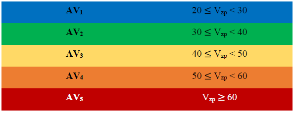
It is known from previous studies that irregularities in the F region can be observed when Vzp amplitudes are higher than 30 m s−1 (Abdu et al., 1985; Fejer et al., 1999). In the Brazilian region, Abdu et al. (1983) and Abdu et al. (2009a) found that the Vzp should be around 30–50 m s−1 to observe the irregularity/spread F. Other authors found a threshold of 40 m s−1 in different locations (Basu et al., 1996; Whalen, 2003). Furthermore, the irregularity occurrence probability becomes higher when the Vzp is greater than 40 m s−1 (Huang et al., 2015). In fact, we do not observe in our analysis an expressive irregularity occurrence for the Vz less than 40 m s−1. Therefore, the threshold was selected as 40 m s−1 here to validate the proposed AV index. In other words, values smaller than 40 m s−1 mean that the irregularity will not appear (AV1) or will rarely appear (AV2) since the interest of this study is related to general cases.
Since the Vzp intensification may indicate the occurrence of plasma irregularities in ionograms, mainly plasma bubbles, we performed a statistical analysis to find a correlation between the instant in which the Vzp increases and the time that the irregularity is identified. An example is shown in Table 2 for 11 January 2001. It is observed that the Vzp reaches 43 m s−1 at 21:45 UTC, corresponding to the AV3 index. The irregularity can be observed in the ionogram 45 min after the Vzp peak (22:30 UTC), as shown in Fig. 1. The red arrows indicate the spread in the F region.
Table 2Example of the relationship between the irregularity occurrence and the Vzp parameter.
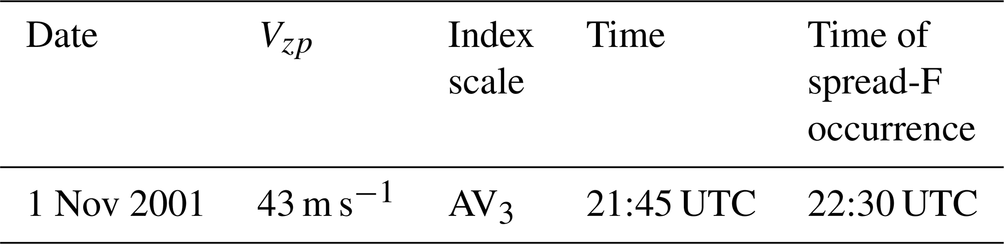

Figure 1Sequences of ionograms showing the spread F over São Luís on 11 January 2001 (red arrows).
3.2 AV index validation
Table 3 presents statistics of the data used in the analysis for 2001 and 2015, considering the total number of observations, number of days in which the irregularities were observed, and the number of days that were classified as the AV3, AV4, or AV5.
Table 3Statistics of the data used in this study for 2001 and 2015.

Figure 2 shows the statistical analysis between the Vzp values considering only the indexes AV3, AV4, and AV5 and the time that the irregularity starts to appear in the ionogram. Firstly, the analysis takes into account the data gathered in the summer of 2001 and 2015 over São Luís. The interval between the Vzp peak and the observation of the spread F was discretized into five intervals for the sake of the analysis: 0, 15, 30, 45, and ≥60 min. This quantity is called the Δtvi hereafter. Notice that this granularity of 150 min is a limitation of the Digisonde sampling time, and all the occurrences in which the Δtvi is higher than 60 min were placed in the last interval.
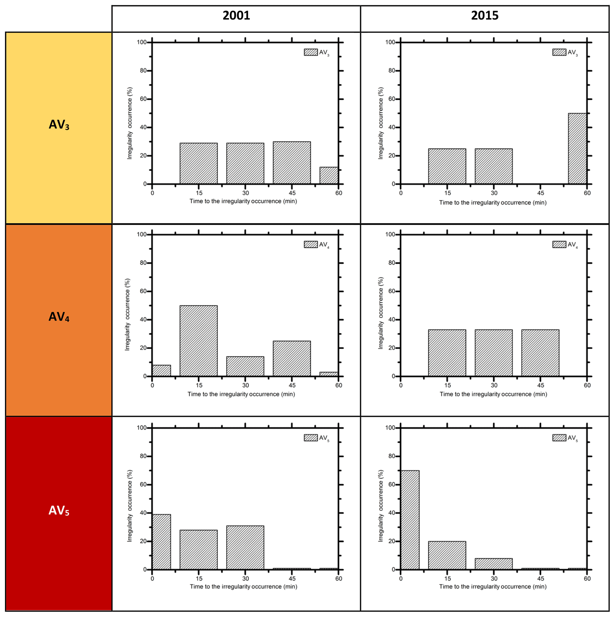
Figure 2The time relationship between the Vzp parameter, considering the AV3, AV4, and AV5 indexes, and the irregularity observations in ionograms in the summer of 2001 and 2015 over São Luís.
Comparing the results for the AV3 index, it is observed that the Δtvi is at least 15 min in both solar cycles. In 2015, no data with the Δtvi equal to 45 min were observed. There was also a significant change comparing both scenarios with respect to the occurrences with the Δtvi equal to or greater than 60 min. In 2001, only 16 % of the cases fell into this interval, whereas in 2015 it was 50 %. The high occurrence in the descending phase of the solar cycle could be related to the post-midnight occurrence of the irregularities and, generally, they are observed in low solar activity (Otsuka, 2018).
Regarding the AV4 index, 10 % of the cases had a Δtvi equal to 0 min during the maximum solar flux (2001), meaning that the spread F occurred at the same time of the Vzp. On the other hand, in 2015 no data fell into this interval. However, notice that there is a high probability that the Δtvi is equal to or higher than 15 min.
When the index reached the AV5 corresponding to extreme cases, we observe a high occurrence of events in which the Δtvi equals 0 min. In fact, notice that almost 40 % of that data in 2001 and 70 % of the data in 2015 comprise this interval.
It can be inferred from our results that the probability density function of the Δtvi for the AV3 and AV4 approaches a uniform distribution with its lower bound at 15 min, except for 2001 and the AV4. Regarding the AV5 in 2001, the distribution seems uniform with its lower bound at 0 min and its upper bound at 30 min. For the same index, the distribution appears to be exponential in 2015. Furthermore, it can be concluded that there is a high probability of observing a Δtvi of less than 15 min, given that the index for the AV3 or AV4 is negligible.
It is well established that the spread-F occurrence depends on the season and epoch in the solar cycle (Abdu et al., 1983, 1995; Abdu, 2001). Abdu et al. (1985) showed that the drift velocities were small during low-sunspot years, which weakens the development of irregularities. Huang et al. (2002) observed that the maximum irregularity rates were significantly higher during the maximum phase of the solar cycle. This behavior happens because the thermospheric winds and longitudinal gradients in conjugate-E layer conductivity are more effective. Those are the key parameters that control the evening F region dynamo electric field. Therefore, during high solar activity, there are significant variations in thermospheric winds and in longitudinal conductivity gradients of the evening conjugate E layers, which lead to higher values of the Vzp and, consequently, a favorable environment for irregularity formation (Abdu et al., 1983).
In our analysis, we observed a significantly high number of irregularities in 2015. We believe that this is caused by the descending phase of the solar cycle. However, although the irregularities reached the AV5 level in 2015, its duration in ionograms was lower than in 2001. This can be seen in Fig. 3, where we show the duration of spread F in ionograms for the AV3 level in 2001 and 2015. The duration of the irregularities was divided into five intervals: less than 6, between 6 and 7, between 7 and 8, between 8 and 9, and more than 9 h (t<6, 6<t<7, 7<t<8, 8<t<9, and ≥9 h). The difference between the years is very clear, and during the high solar cycle the duration of the irregularities is more than 9 h for most of the events. On the other hand, in 2015 the spread F lasted less than 6 h in almost 70 % of cases, revealing a solar flux influence and agreeing with the previous study (Abdu et al., 1985; Huang et al., 2002).
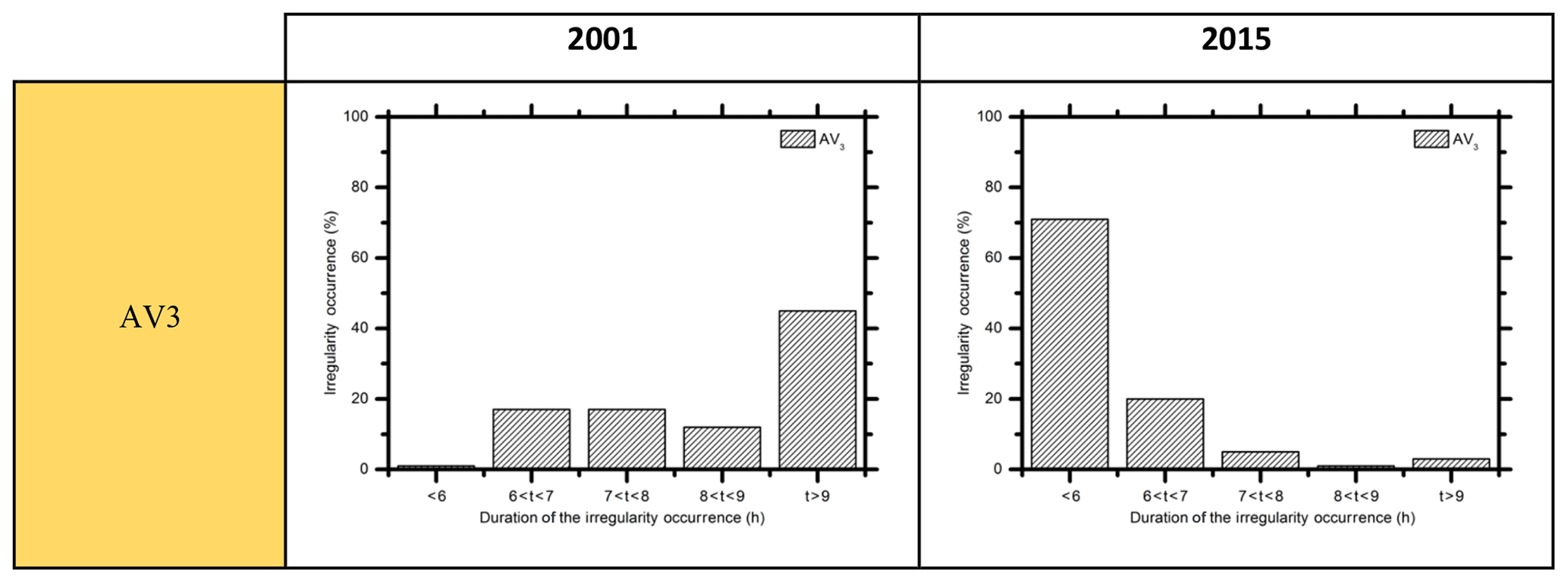
Figure 3Occurrence of spread F in ionograms for the AV3 index in 2001 and 2015 over São Luís to exemplify the differences between the solar flux levels.
In the early hours, the irregularities were controlled by the polarization electric field, but after 6 h the ionospheric plasma dynamics control the bubble (Huang et al., 2011). Barros et al. (2018) show an important role of the zonal wind plays in the evolution of the plasma bubbles in the TEC data between 2012 and 2016. They did not discuss the differences in the solar cycle phases. However, they showed a good agreement between the zonal drift velocities and the thermospheric winds regarding the occurrence of plasma bubbles. Therefore, we believe that the thermospheric winds in 2015 were lower than in 2001, interfering with the growth rate of Rayleigh–Taylor instability (discussed below). This fact will be evaluated in greater detail in future work.
As mentioned before, the spread F is directly related to the plasma bubbles. These plasma bubbles are formed due to the Rayleigh–Taylor gravitational instability process, which is operational on the steep upward gradient in the nighttime bottom side of the F region at the magnetic equator (Abdu et al., 2006). This Rayleigh–Taylor mechanism is related to the linear growth rate (γ) given by Haerendel et al. (1992), Sultan (1996), and Abdu et al. (2009a, 2006).
where the ∑P is the Pedersen conductivity in the field line integrated for E and F, UP is the Pedersen conductivity-weighted neutral wind perpendicular to the magnetic field in the magnetic meridian plane, E and B are the intensities of the ambient zonal electric field and the magnetic field, g is the gravitational acceleration, ν is the collision frequency, L is the McIlwain parameter, and β is the recombination loss rate. All the terms in this equation were discussed in Abdu (2001). However, we highlight here that the angle formed between the solar terminator and the magnetic meridian is relatively small in summer, and consequently there is an almost instantaneous decoupling between the E and F regions (Batista et al., 1986). Thus, the polarization electric fields of the F region associated with the Vz peak have higher amplitudes, favoring instability growth. Thus, the irregularity is more favored to occur in summer than winter (Tsunoda, 1985; Barros et al., 2018).
In order to investigate the seasonal behavior, we analyzed the AV index for the equinoxes and the winter of 2001 and 2015 over São Luís. The results are presented in Figs. 4 and 5 for the equinoxes and winter, respectively.
In relation to the equinoxes (Fig. 4), the Vzp did not reach the AV5 in both years. For the AV4, only a few cases were observed in the high solar cycle. Among those, 10 % had a Δtvi equal to 0 min, 34 % had a Δtvi equal to 15 min, 15 % had a Δtvi equal to 30 min, 10 % had a Δtvi equal to 45 min, and 31 % had a Δtvi equal to or greater than 60 min. Regarding the AV3, the irregularities were observed between 15 and 45 min after the Vzp peak in both years. No significant values in which the Δtvi was equal to 0 min or greater than 60 min were found.
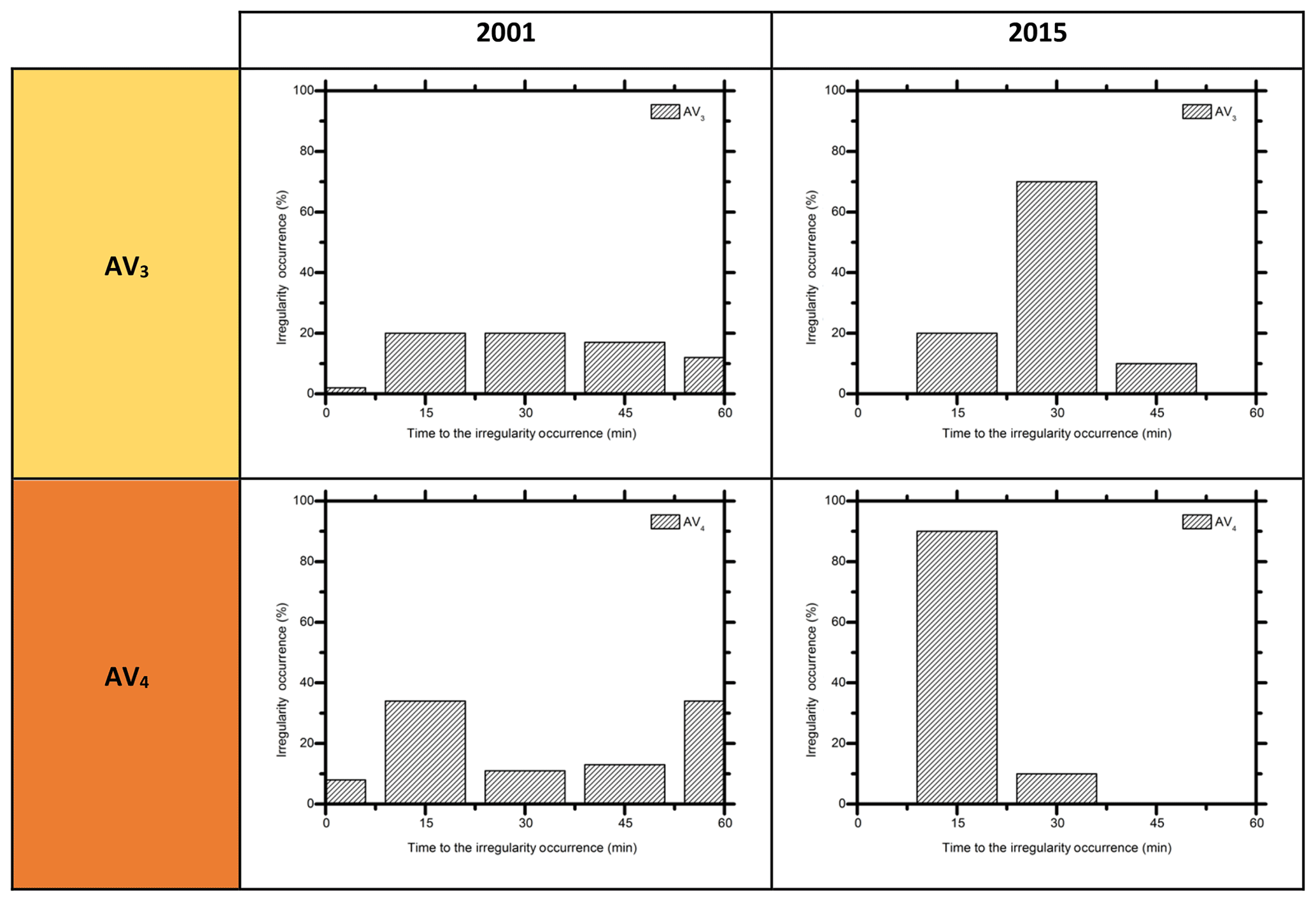
Figure 4The time relationship between the Vzp parameter, considering the AV3 and AV4 indexes, and the irregularity observations in ionograms in the equinoxes of 2001 and 2015 over São Luís. The Vzp did not reach the AV5 scale.
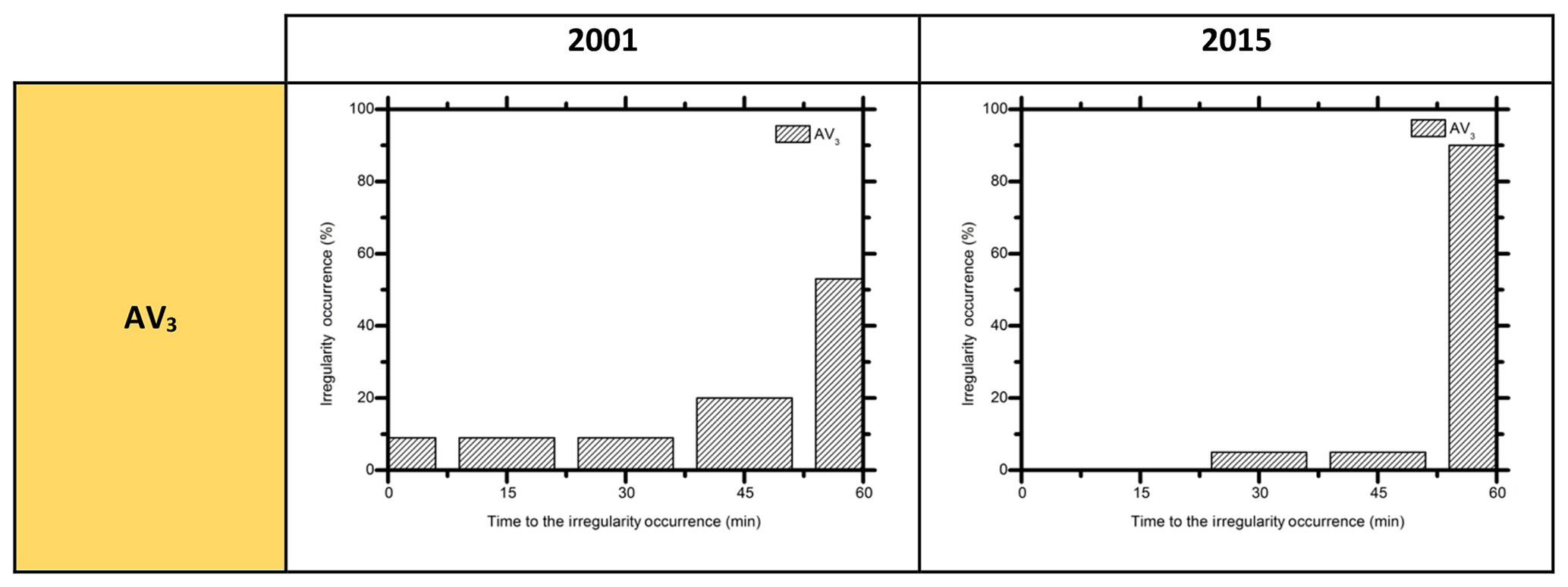
Figure 5The time relationship between the Vzp parameter, considering the AV3 index, and the irregularity observations in ionograms in the winter of 2001 and 2015 over São Luís. The Vzp did not reach the AV4 and AV5 scales.
As seen in Fig. 5, the index did not reach the AV4 or the AV5 in winter. During the high solar cycle, 10 % of the cases had a Δtvi equal to 0 min, 10 % had a Δtvi equal to 15 min, 10 % had a Δtvi equal to 30 min, and almost 20 % had a Δtvi equal to 45 min. Thus, most of the irregularity observations occurred after 1 h from the Vzp peak. In general, the irregularities observed in the ionograms had a Δtvi equal to or greater than 60 min in 2015.
Therefore, we observed only a few cases of spread F in both seasons, agreeing with previous studies that irregularities related to plasma bubbles are more frequent in summer (Barros et al., 2018). Thus, we considered the analysis of the summer as enough to validate the proposed AV scale. However, it is important to mention that the index is valid for the other stations of the year too, as shown in the examples above. The climatological results are presented in the following section.
3.3 Climatological study of the AV index and spread F in summer
Figure 6 shows the relationship between Vzp intensification, the AV index, and the time that the irregularity starts to appear in the ionogram. This study considered the data obtained from São Luís station from the summer of 2009 to 2014. The years 2009 and 2010 occurred during the minimum solar cycle 24, 2011 and 2012 occurred during the ascending phase of the same solar cycle, and 2013 and 2014 occurred during its maximum. In this figure, we also show the quantity of available observations and the number of days that we used in the analysis (below the year). Also, we show the quantity for each scale in the AV index used in this analysis.
It is possible to observe from the results that there is no regular pattern between the highest Vzp value and the irregularity observations. However, it is important to mention that the probability to observe a Δtvi equal to or higher than 15 min is still very high in all phases of the solar cycle.
After the AV3 and AV4 results, we did not observe significant values with a Δtvi equal to 0 min. Most of the events found that the Δtvi lies between 30 min and greater than 60 min, showing the same pattern of the results presented in the previous section. Additionally, a high number of observations with a Δtvi greater than 60 min were found, mainly in 2009, 2010, and 2014. As mentioned before, this percentage can be associated with the irregularities that occurred in the post-midnight hours, which is a common observation in low solar activity. Otsuka (2018) affirms that during solar minimum conditions, post-midnight irregularities may occur mostly in association with plasma bubbles initiated around midnight. In addition, post-midnight plasma bubbles could be caused by atmospheric gravity wave seeding of Rayleigh–Taylor instability and/or an increase in the growth rate of Rayleigh–Taylor instability due to F-layer uplift.
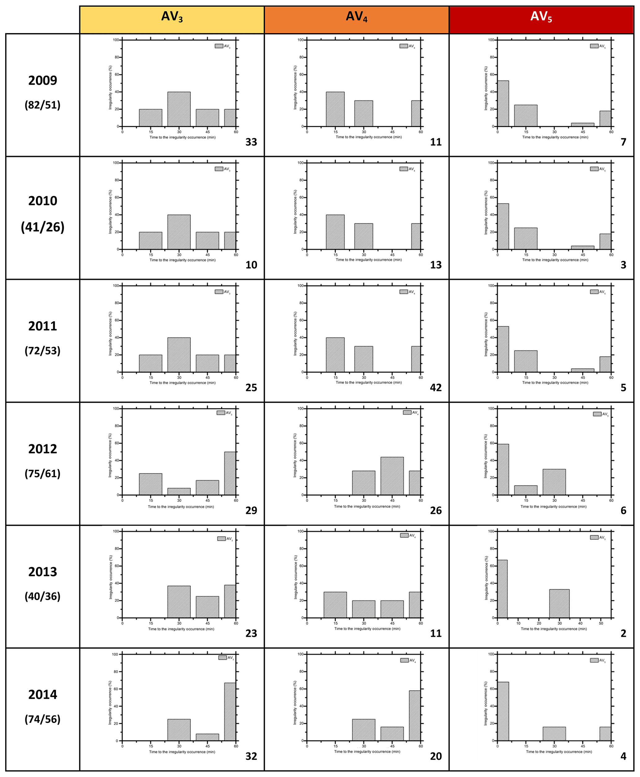
Figure 6The time relationship between the Vzp parameter, considering the AV3, AV4, and AV5 indexes, and the irregularity observations in ionograms in the summer of 2009 until 2014 over São Luís.
We notice that when the index reached the AV5, there is a high occurrence of events with a Δtvi equal to 0 min. This behavior is clearly observed during the ascending and maximum phases of the solar cycle, which accounts for almost 70 % of the occurrences in this interval. During the minimum solar cycle (2009 and 2010), this probability for such occurrences reduces to less than 60 %. This fact can serve as evidence that the zonal drift reversal time and the weak zonal neutral wind magnitude can cause a delay in the irregularity occurrence during the solar minimum activity phase (Abdu et al., 1985). Despite all these promising results, we shall recall that we are working with a 7-year interval. Thus, any definitive conclusion on the solar cycle dependence must be accompanied by a more comprehensive study that confirms our results.
We included an analysis of the average Δtvi considering all the years for the AV3 (yellow line), AV4 (orange line), and AV5 (red line) in Fig. 7. It is possible to observe that the mean Δtvi is greater than 60 min for the AV3 and AV4. In severe events, i.e., AV5, we had the mean Δtvi equal to 0 min. Thus, we can infer that, with considerable probability (around 50 %), regarding the AV3 and AV4, the elapsed time between the Vzp peak and the irregularity occurrence is greater than 60 min.
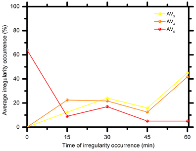
Figure 7The average time relationship between the Vzp parameter, considering the AV3 (yellow), AV4 (orange), and AV5 (red) indexes, and the irregularity observations in ionograms in summer from 2009 until 2014 over São Luís.
It is well known that the term in Eq. (1) arises from the evening vertical drift enhancement, also known as PRE (Abdu et al., 2009b). Therefore, when the base of the F layer lies above 300 km, is approximately equal to the Vzp (Bittencourt and Abdu, 1981; Batista et al., 1986). Furthermore, the term can be enhanced due to a large Vzp, leading to an enhancement of the linear growth rate (γ). In other words, there is a clear compromise between the Vzp and the linear growth rate of the plasma bubble. Moreover, several authors have reported the necessity to have a wave-like perturbation to trigger Rayleigh–Taylor instability (Abdu et al., 2009b; Takahashi et al., 2018; Tsunoda, 2006).
Using data from ground-based experiments conducted during the 2005 SpreadFEx campaign in Brazil, Abdu et al. (2009c) have shown a few case studies where it is possible to identify a relationship between the Vzp and plasma bubble occurrence. The authors observed that the spread F occurs 30 min after the Vzp reached values of around 40 m s−1. They concluded that the relationship between the Vzp and plasma bubble occurrence is a significant factor in understanding the development of these irregularities. Moreover, as mentioned before, several authors have reported the necessity to have a wave-like perturbation trigger Rayleigh–Taylor instability, which is responsible for plasma irregularity formation in the F region (Abdu et al., 2009c; Tsunoda, 2006). Narayanan et al. (2014) studied the connection between the equatorial spread F and satellite traces over an Indian equatorial station, Tirunelveli (8.7∘ N, 77.8∘ E; dip: 1.1∘ N). They used ionosonde observations with 5 min intervals from March 2008 to February 2009 during the extended solar minimum conditions. Among their results, they found an average spread-F onset delay of about 30 min compared to observations made with the satellite traces. Therefore, they believed that the satellite trace remarks may be used as a precursor to irregularity occurrences. Additionally, they recommended validating their analysis with the Vzp parameter, but they did not perform this analysis.
In a recent study, Sousasantos et al. (2019) developed a three-dimensional numerical model to analyze plasma bubble structure. An input parameter is the PRE (ranging between 20 and 60 m s−1) obtained using the SAMI2 model (Huba et al., 2000), which is a necessary condition in addition to all mechanisms in forming plasma bubbles. Thus, the authors showed that the plasma bubble structure is generated approximately 20–30 min after the PRE enters in the model. They attributed this delay to the parallel conductivity that may reduce the growth rate on the equatorial region. In turn, this implies longer times are required to reach the nonlinear stage.
As presented here, the relationship between the Vzp and irregularity onset time is an open important scientific issue. Based on the previous studies, both wave-like perturbations or parallel conductivity can modify the outset of the irregularity, being the responsible for the delay. In order to determine the key factor, a more comprehensive and specific study shall be designed.
Additionally, the ionospheric indexes found show a relationship between TEC or satellite measurements and plasma irregularity occurrence (Huang et al., 2015; Nishioka et al., 2017). On the other hand, there is no ionospheric index in the available literature that found a relationship between the drift velocity and irregularity/plasma bubble occurrences. Furthermore, this study confirms that this proposed index can be used to warn users about irregularity occurrences, since it was shown that regarding the AV3 and AV4 there is at least 15 min between observation of the Vzp peak and the occurrence of the irregularity.
Finally, as a perspective for future work, this index will be useful to study the seasonality, solar cycle, and onset time of plasma irregularities. Notice that the temporal error is around 15 min, since the ionograms have this range of time. However, we believe that the error is not significant in terms of spread-F occurrence. Therefore, the AV index is suitable to be incorporated into the products offered by the Embrace program, and it will help in the evaluation of phenomena impacts in the space weather environment.
In this study, we develop an ionospheric index, AV, based on the Vz parameter in the F region. The index quantifies the time relationship between the Vzp and the ionospheric irregularity occurrences that may be associated with plasma bubbles, Δtvi. We analyzed data from 2 years, 2001 and 2015, representing different solar flux in order to construct the AV index scale. After, we performed a climatological study from 2009 to 2014, in order to validate the AV scale.
In general, the results show that a Δtvi is at least 15 min in both solar cycles for the AV3 and AV4 indexes. However, when the index reached the AV5, in which case it is considered an extreme event, we observed a rate of events with a Δtvi equal to 0 min (60 % of the cases).
Additionally, we observed a significantly high number of irregularities in 2015 (61 cases in summer, 58 during the equinoxes, and 23 in winter). We attributed this fact to the descending phase of the solar cycle. However, although the irregularities reached the AV5 in 2015, its duration in ionograms was lower than in 2001. We believe that the thermospheric winds are the main agent responsible for this behavior, since they interfere in the growth rate of Rayleigh–Taylor instability. This fact will be evaluated in greater detail in future work.
We performed a climatological study during the summer since this season is more significant regarding spread-F occurrences. Thus, we considered the data obtained from the São Luís station from 2009 to 2014, almost covering the ascending solar cycle. We show an irregular pattern between the highest Vzp value and irregularity observations. However, it is important to mention that the probability to observe a Δtvi equal to or higher than 15 min is still very high in all phases of the solar cycle. In fact, we can infer that, with very high probability under the AV3 and AV4, the elapsed time between the Vzp peak and the irregularity occurrence is greater than 60 min.
Finally, as stated in previous studies the wave-like perturbations which trigger Rayleigh–Taylor instability or parallel conductivity can modify the outset of the irregularity, and this might be responsible for the delay between the Vzp and irregularity occurrence. However, more studies are needed to understand this relationship. In fact, we did not find any study about the ionospheric index that showed the relationship between the drift velocity and irregularity/plasma bubble occurrences that is shown in this work. Thus, the AV index is suitable to be incorporated into the products offered by the Embrace program, and it will help in the evaluation of phenomena impacts in the space weather environment.
The data used in this study are available by contacting the Responsible Coordinator at the DAE/INPE (Inez S. Batista, email: inez.batista@inpe.br).
LCAR, CMD, GP, DB, and CF designed the study, analyzed and interpreted the data, and wrote the paper. JM and RP helped to improve the paper. All authors read and approved the paper
The authors declare that they have no conflict of interest.
This article is part of the special issue “7th Brazilian meeting on space geophysics and aeronomy”. It is a result of the Brazilian meeting on Space Geophysics and Aeronomy, Santa Maria/RS, Brazil, 5–9 November 2018.
Laysa Cristina Araujo Resende would like to thank the National Space Science Center (NSSC), the Chinese Academy of Sciences (CAS) for supporting her postdoctoral research, and the CNPq/MCTIC (grant no. 169404/2017-0). Clezio Marcos Denardini thanks the CNPq/MCTI (no. grant 03121/2014-9). Giorgio Arlan Silva Picanço would like to thank the CNPq for the financial support received during his M.Sc. (grant no. 132252/2017-18). Juliano Moro would like to thank the National Space Science Center (NSSC), the Chinese Academy of Sciences (CAS) for supporting his postdoctoral research, and the CNPq/MCTIC (grant no. 429517/2018-01). Diego Barros thanks the CNPq for his fellowship (grant no. 301211/2019-1). Cosme Alexandre Oliveira Barros Figueiredo thanks the FAPESP for his postdoctoral fellowship (grant no. 2018/09066-8). Régia Pereira Silva thanks the CNPq for their support (grant no. 300329/2019-9). The authors thank DAE/INPE for kindly providing the ionospheric data.
This paper was edited by Igo Paulino and reviewed by Ricardo Cueva and one anonymous referee.
Abdu, M. A.: Outstanding problems in the equatorial ionosphere- thermosphere electrodynamics relevant to spread F, J. Atmos. Terr. Phys., 63, 869–884, https://doi.org/10.1016/S1364-6826(00)00201-7, 2001.
Abdu, M. A., Medeiros, R. T., Bittencourt, J. A., and Batista, I. S.: Vertical ionization drift velocities and range spread F in the evening equatorial ionosphere, J. Geophys. Res., 88, 399–402, https://doi.org/10.1029/JA088iA01p00399, 1983.
Abdu, M. A., Sobral, J. H. A., Nelson, O. R., and Batista, I. S.: Solar cycle related range type spread-F occurrence characteristics over equatorial and low latitude stations in Brazil, J. Atmos. Terr. Phys., 47, 901–905, https://doi.org/10.1016/0021-9169(85)90065-0, 1985.
Abdu, M. A., Batista, I. S., Walker, G. O., Sobral, J. H. A., Trivedi, N. B., and De Paula, E. R.: Equatorial Ionospheric Electric Fields During Magnetospheric Disturbances: Local Time/Longitude Dependences from Recent EITS Campaigns, J. Atmos. Terr. Phys., 57, 1065–1083, https://doi.org/10.1016/0021-9169(94)00123-6, 1995.
Abdu, M. A., Batista, P. P., Batista I. S., Brum, C. G. M., Carrasco, A. J., and Reinisch, B. W.: Planetary wave oscillations in mesospheric winds, equatorial evening prereversal electric field and spread F, Geophys. Res. Lett., 33, 1–4, https://doi.org/10.1029/2005GL024837, 2006.
Abdu, M., Kherani, A. E. A., Batista, I. S., and Sobral, J. H. A.: Equatorial Evening Prereversal Vertical Drift and Spread F Suppression by Disturbance Penetration Electric Fields, Geophys. Res. Lett., 36, L19103, https://doi.org/10.1029/2009GL039919, 2009a.
Abdu, M. A., Alam Kherani, E., Batista, I. S., de Paula, E. R., Fritts, D. C., and Sobral, J. H. A.: Gravity wave initiation of equatorial spread F/plasma bubble irregularities based on observational data from the SpreadFEx campaign, Ann. Geophys., 27, 2607–2622, https://doi.org/10.5194/angeo-27-2607-2009, 2009b.
Abdu, M. A., Batista, I. S., Reinisch, B. W., de Souza, J. R., Sobral, J. H. A., Pedersen, T. R., Medeiros, A. F., Schuch, N. J., de Paula, E. R., and Groces, K. M.: Conjugate Point Equatorial Experiment (COPEX) campaign in Brazil: Electrodynamics highlights on spread F development conditions and day-to-day variability, J. Geophys. Res., 114, A04308, https://doi.org/10.1029/2008JA013749, 2009c.
Barros, D., Takahashi, H., Wrasse, C. M., and Figueiredo, C. A. O. B.: Characteristics of equatorial plasma bubbles observed by TEC map based on ground-based GNSS receivers over South America, Ann. Geophys., 36, 91–100, https://doi.org/10.5194/angeo-36-91-2018, 2018.
Basu, S., Kudeki, E., Valladares, C. E., Weber E. J., Zengingonul, H. P., Bhattacharyya, S., Sheehan, R., Meriwether, J. W., Biondi, M. A., Kuenzler, H., and Espinoza, J.: Scintillations, plasma drifts, and neutral winds in the equatorial ionosphere after sunset, J. Geophys. Res., 101, 795–809, https://doi.org/10.1029/96JA00760, 1996.
Batista, I. S., Abdu, M. A., and Bittencourt, J. A.: Equatorial F-region vertical plasma drifts: Seasonal and Longitudinal Asymmetries in the American Sector, J. Geophys. Res., 91, 12055–12064, https://doi.org/10.1029/JA091iA11p12055, 1986.
Batista, I. S., De Medeiros, R. T., Abdu, M. A., De Sousa, J. R., Bailey, G. J., and De Paula, E. R.: Equatorial ionosphere vertical plasma drift model over the Brazilian region, J. Geophys. Res., 101, 10887–10892, https://doi.org/10.1029/95JA03833, 1996.
Bittencourt, J. A. and Abdu, M. A.: Theoretical Comparison between Apparent and Real Vertical Ionization Drift Velocities in the Equatorial F-Region, J. Geophys. Res., 86, 2451–55, https://doi.org/10.1029/JA086iA04p02451, 1981.
Farley, D. T., Bonelli, E., Fejer, B. G., and Larsen, M. F.: The prereversal enhancement of the zonal electric field in the equatorial ionosphere, J. Geophys. Res., 91, 13723–13728, https://doi.org/10.1029/JA091iA12p13723,1986.
Fejer, B. G.: Low latitude electrodynamic plasma drifts: A review, J. Atmos. Terr. Phys., 53, 677–693, https://doi.org/10.1016/0021-9169(91)90121-M, 1991.
Fejer, B. G., Farley, D. T., Woodman, R. F., and Calderon, C.: Dependence of equatorial F region vertical drifts on season and solar cycle, J. Geophys. Res., 84, 5792–5796, https://doi.org/10.1029/JA084iA10p05792, 1979.
Fejer, B. G., Scherliess, L., and De Paula, E. R.: Effects of the vertical plasma drift velocity on the generation and evolution of equatorial spread F, J. Geophys. Res., 104, 19854–19869, https://doi.org/10.1029/1999JA900271, 1999.
Fejer, B. G., Jensen, J. W., and Su, S. Y.: Seasonal and longitudinal dependence of equatorial disturbance vertical plasma drifts, Geophys. Res. Lett., 35, L20106, https://doi.org/10.1029/2008GL035584, 2008.
Haerendel, G., Eccles, J., and Cakir, S.: Theory of modeling the equatorial evening ionosphere and the origin of the shear in the horizontal plasma flow, J. Geophys. Res., 97, 1209–1223, https://doi.org/10.1029/91JA02226, 1992.
Heelis, R. A., Kendall, P. C., Moffet, R. J., Windle, D. W., and Rishbeth, H.: Electrical coupling of the E- and F-region and its effects on the F-region drifts and winds, Planet. Space Sci., 22, 743–756, https://doi.org/10.1016/0032-0633(74)90144-5, 1974.
Huang, C. Y., Burke, W. J., Machuzak, J. S., Gentile, L. C., and Sultan, P. J.: Equatorial plasma bubbles observed by DMSP satellites during a full solar cycle: Toward a global climatology, J. Geophys. Res., 107, 1434, 1–10, https://doi.org/10.1029/2002JA009452, 2002.
Huang, C. S., Beaujardiere, O., Roddy, P. A., Hunton, D. E., Pfaff, R. F., Valladares, C. E., and Ballenthin, J. O.: Evolution of equatorial ionospheric plasma bubbles and formation of broad plasma depletions measured by the C/NOFS satellite during deep solar minimum, J. Geophys. Res.-Space, 116, A03309, https://doi.org/10.1029/2010JA015982, 2011.
Huang, C. S. and Hairston, M. R.: The post-sunset vertical plasma drift and its effects on the generation of equatorial plasma bubbles observed by the C/NOFS satellite, J. Geophys. Res.-Space, 120, 2263–2275, https://doi.org/10.1029/2010JA015982, 2015.
Huba, J., Joyce, G., and Fedder, J. A.: Sami2 is Another Model of the Ionosphere (SAMI2): a new low-latitude ionosphere model, J. Geophys. Res.-Space, 105, 23035–23053, https://doi.org/10.1029/2000JA000035, 2000.
Jakowski, N., Borries, C., and Wilken, V.: Introducing a disturbance ionosphere index, Radio Sci., 47, RS0L14, https://doi.org/10.1029/2011RS004939, 2012.
Narayanan, V. L., Sau, S., Gurubaran, S., Shiokawa, K., Balan, N., Emperumal, K., and Sripathi, S.: A statistical study of satellite traces and evolution of equatorial spread F, Earth Planet. Space, 66, 1–13, 2014.
Nishioka, M., Tsugawa, T., Jin, H., and Ishii, M.: A new ionospheric storm scale based on TEC and foF2 statistics, Space Weather, 15, 228–239, https://doi.org/10.1002/2016SW001536, 2017.
Otsuka, Y.: Review of the generation mechanisms of post-midnight irregularities in the equatorial and low-latitude ionosphere, Prog. Earth Planet. Sci., 5, 1–13, https://doi.org/10.1186/s40645-018-0212-7, 2018.
Reinisch, B. W.: New techniques in ground-based ionospheric sounding and studies, Radio Sci., 21, 331–341, https://doi.org/10.1029/RS021i003p00331, 1986.
Reinisch, B. W., Galkin, I. A., and Khmyrov, G. M.: New Digisonde for research and monitoring applications, Radio Sci., 44, RS0A24, https://doi.org/10.1029/2008RS004115, 2009.
Sousasantos, J., Kherani, E. A., Sobral, J. H. A., Abdu, M. A., Moraes, A. O., and Oliveira, C. B. A.: A numerical study on the 3-D approach of the equatorial plasma bubble seeded by the prereversal vertical drift, J. Geophys. Res.-Space, 124, 4539–4555, https://doi.org/10.1029/2018JA026239, 2019
Sultan, P. J.: Linear theory and modeling of the Rayleigh–Taylor instability leading to the occurrence of equatorial spread F, J. Geophys. Res., 101, 26875–26891, https://doi.org/10.1029/96JA00682, 2006.
Takahashi, H., Wrasse, C. M., Figueiredo, C. A. O. B., Barros, D., Abdu, M. A., Otsuka, Y., and Shiokawa, K.: Equatorial plasma bubble seeding by MSTIDs in the ionosphere, Prog. Earth Planet. Sci., 32, 1–13, https://doi.org/10.1186/s40645-018-0189-2, 2018.
Tsunoda, R. T.: Control of the seasonal and longitudinal occurrence of equatorial scintillation by longitudinal gradient in integrated Pedersen conductivity, J. Geophys. Res., 90, 447–456, https://doi.org/10.1029/JA090iA01p00447, 1985.
Tsunoda, R. T.: Day-to-day variability in equatorial spread F: Is there some physics missing?, Geophys. Res. Lett., 33, L16106, https://doi.org/10.1029/2006GL025956, 2006.
Whalen, J. A.: Dependence of the equatorial anomaly and of equatorial spread F on the maximum prereversal E×B drift velocity measured at solar maximum, J. Geophys. Res., 108, 1193, https://doi.org/10.1029/2002JA009755, 2003.