the Creative Commons Attribution 4.0 License.
the Creative Commons Attribution 4.0 License.
 | 12 Aug 2019
High-resolution vertical total electron content maps based on multi-scale B-spline representations
Michael Schmidt
Eren Erdogan
Barbara Görres
Florian Seitz
For more than 2 decades the IGS (International GNSS Service) ionosphere associated analysis centers (IAACs) have provided global maps of the vertical total electron content (VTEC). In general, the representation of a 2-D or 3-D function can be performed by means of a series expansion or by using a discretization technique. While in the latter case, pixels or voxels are usually chosen for a spherical function such as VTEC, for a series expansion spherical harmonics (SH) are primarily used as basis functions. The selection of the best suited approach for ionosphere modeling means a trade-off between the distribution of available data and their possibility of representing ionospheric variations with high resolution and high accuracy.
Most of the IAACs generate global ionosphere maps (GIMs) based on SH expansions up to the spectral degree n=15 and provide them with a spatial resolution of with respect to the latitudinal and longitudinal directions, respectively, and a temporal sampling interval of 2 h. In recent years, it has frequently been claimed that the spatial resolution of the VTEC GIMs has to be increased to a spatial resolution of and to a temporal sampling interval of about 15 min. Enhancing the grid resolution means an interpolation of VTEC values for intermediate points but with no further information about variations in the signal. n=15 in the SH case, for instance, corresponds to a spatial sampling of . Consequently, increasing the grid resolution concurrently requires an extension of the spectral content, i.e., to choose a higher SH degree value than 15.
Unlike most of the IAACs, the VTEC modeling approach at Deutsches Geodätisches Forschungsinstitut der Technischen Universität München (DGFI-TUM) is based on localizing basis functions, namely tensor products of polynomial and trigonometric B-splines. In this way, not only can data gaps be handled appropriately and sparse normal equation systems be established for the parameter estimation procedure, a multi-scale representation (MSR) can also be set up to determine GIMs of different spectral content directly, by applying the so-called pyramid algorithm, and to perform highly effective data compression techniques. The estimation of the MSR model parameters is finally performed by a Kalman filter driven by near real-time (NRT) GNSS data.
Within this paper, we realize the MSR and create multi-scale products based on B-spline scaling, wavelet coefficients and VTEC grid values. We compare these products with different final and rapid products from the IAACs, e.g., the SH model from CODE (Berne) and the voxel solution from UPC (Barcelona). In contrast to the abovementioned products, DGFI-TUM's products are based solely on NRT GNSS observations and ultra-rapid orbits. Nevertheless, we can conclude that the DGFI-TUM's high-resolution product (“othg”) outperforms all products used within the selected time span of investigation, namely September 2017.
- Article
(4754 KB) - Full-text XML
- BibTeX
- EndNote


The properties of the atmosphere can be described by means of different variables, e.g., the temperature or the charge state. In the case of temperature, we distinguish between the troposphere (up to a height of about 15 km), the stratosphere (about 15 to 50 km), the mesosphere (about 50 to 90 km), the thermosphere (about 90 to 800 km) and the exosphere (above 800 km) using increasing height above the Earth's surface. In the case of the charge state, the atmosphere is split into the neutral atmosphere (up to a height of 80 km), the ionosphere (about 80 to 1000 km) and the plasmasphere (above 1000 km) (see, e.g., Limberger, 2015).
The ionosphere is mostly driven by the Sun; extreme UV (EUV), X-ray and solar particle radiation cause ionization processes. In geodesy, the main ionospheric impact is the influence of free electrons on radio wave propagation. This effect mainly depends on the signal frequency, i.e., the ionosphere is a dispersive medium (Schaer, 1999). Signals with frequencies lower than 30 MHz will be blocked and reflected by the ionosphere, whereas signals with shorter wavelengths penetrate the ionosphere but are affected with respect to speed and direction. The ionospheric influence on radio waves is twofold: the signal travel times are changed (delay) and the signal paths are modified (bending). While the latter effect can be neglected for most applications, the ionospheric delay
depends directly on the electron density Ne along the signal path s between satellite S and receiver R and inversely on the carrier frequency f. Equation (1), which can be derived from dual-frequency measurements, is only an approximation as higher-order effects are neglected. These terms depend on the magnetic field, signal frequency, signal elevation, and ionospheric conditions and reach about 0.2 cm in zenith for GPS signals (Bassiri and Hajj, 1993). The sign on the right-hand side changes depending on whether it is applied for a carrier phase observation (“−”) or for a pseudorange measurement (“+”) (see, e.g., Langley, 1998).
Observations of space geodetic techniques, such as the global navigation satellite systems (GNSS) and the Doppler Orbitography and Radiopositioning Integrated by Satellite (DORIS) tracking system as well as satellite altimetry and ionospheric radio occultation (IRO) are based on electromagnetic signal propagation; thus, they are disturbed by the ionosphere. Most of the techniques are not directly sensitive to the electron density, but to the integrated effect along the ray path. In Eq. (1) the integral
is called the slant total electron content (STEC). In Eq. (2), in addition to the time t we introduce the position vectors xS xR and
of the satellite S, the receiver R and an arbitrary point P moving along the signal path s; the coordinate triple comprises latitude φ, longitude λ and radial distance r within a geocentric coordinate system ΣE.
The vertical total electron content (VTEC),
is defined as the integration of the electron density in the vertical direction, i.e., along the height h above the Earth's surface, defined as ; RE refers to the radius of a spherical Earth. Furthermore, in Eq. (4) hl and hu are the respective heights of the lower and the upper boundary of the ionosphere (see, e.g., Dettmering et al., 2011, 2014; Limberger, 2015).
Equations (2) and (4) require a 3-D integration of the electron density. Often a simplification is preferred which is based on the so-called single-layer model (SLM). It assumes that all free electrons are concentrated in an infinitesimally thin shell, i.e., the sphere ΩH with radius (Schaer, 1999), where H is the single-layer height. As a consequence of this assumption and according to
VTEC can be transformed into STEC by introducing a mapping function M(z) depending on the zenith angle z of the ray path between satellite S and receiver R. In Eq. (5) the position vector xIPP, i.e., the spherical coordinates (φIPP, λIPP, RH) define the ionospheric pierce point (IPP), which refers to the geometrical piercing point of the straight line between S and R with the sphere ΩH of the SLM. This point denotes the reference point of an observation including the STEC, such as a GNSS measurement (see, e.g., Erdogan et al., 2017). Figure 1 shows, for instance, the global distribution of the IPPs from GNSS observations on 6 September 2017 between 12:55 and 13:05 UT. However, it must be pointed out that the introduction of a simple isotropic mapping function M(z), depending solely on the zenith angle z, can only generate an approximation of STEC. Recently, more sophisticated approaches, e.g., the Barcelona ionospheric mapping function (BIMF), have been developed to improve the projection of VTEC on STEC (see, e.g., Lyu et al., 2018).
Combining Eqs. (1), (2) and (5) yields the relation
between VTEC and the ionospheric delay dion in the case of a phase observation. Equation (6) can be interpreted and applied in two ways:
-
if VTEC is given from an ionospheric model, the delay dion can be computed and used as a correction for GNSS observations;
-
or if the delay dion can be derived from double-frequency GNSS measurements, it can be used as an observation to develop or improve VTEC models.
Applications, such as satellite navigation and positioning require high-precision and high-resolution VTEC models. For this purpose the correction dion could, according to Eq. (6), be derived from VTEC maps, usually the so-called global ionosphere maps (GIM). The most prominent GIM is provided by the International GNSS Service (IGS) (Feltens and Schaer, 1998; Hernández-Pajares et al., 2011) as a weighted combination product of VTEC maps from various IGS ionosphere associated analysis centers (IAACs), namely (1) the Jet Propulsion Laboratory (JPL), (2) the Center for Orbit Determination in Europe (CODE), (3) the European Space Operations Center of the European Space Agency (ESOC), (4) the Universitat Politècnica de Catalunya (UPC), (5) the Canadian Geodetic Survey of Natural Resources Canada (NRCan), (6) the Wuhan University (WHU) and (7) the Chinese Academy of Sciences (CAS). Recently, Roma-Dollase et al. (2017) published a review paper on these seven GIMs concerning their mapping techniques and their consistency during one solar cycle.
There are several modeling strategies for generating GIMs; the most prominent approach is based on spherical harmonics (SH) and was introduced by Schaer (1999). Further approaches include the tomographic approach based on voxels (Hernández-Pajares et al., 1999) and other approaches based on B-spline scaling functions and wavelets (Schmidt, 2007, 2015b; Schmidt et al., 2011), multivariate adaptive regression splines (MARS) and adaptive regression B-splines (BMARS) (Durmaz et al., 2010; Durmaz and Karslioglu, 2015), and polynomials (Komjathy and Langley, 1996).
Generally, we distinguish between GIMs provided as “final”, “rapid”, “near real-time” (NRT) or “real-time” (RT) products. This classification is based on the latency of the underlying input data. For final products, for instance, only post-processed observations and orbits are used, whereas NRT products are based on rapid orbits and observations with a latency of some minutes up to a few hours. GIMs are typically provided with a temporal resolution of 1 or 2 h and with a spatial resolution of with respect to geographical latitude and longitude (Hernández-Pajares et al., 2017).
VTEC variations basically follow annual, seasonal, diurnal and semidiurnal periods. Earthquakes or incidental natural hazards can also cause small but visible signatures (Liu et al., 2004; Zhu et al., 2013). However, during space weather events, such as solar flares or coronal mass ejections (CME), the number of free electrons may drastically increase. In the latter case, solar plasma consisting of electrons, ions and photons may enter the Earth's atmosphere and cause short period variations within the electron density distribution (see, e.g., Monte-Moreno and Hernández-Pajares, 2014; Wang et al., 2016; Tsurutani et al., 2006, 2009). As a consequence, the modeling of the disturbed ionosphere requires both a high temporal and a high spatial resolution. In 2012, during the IGS 2012 workshop in Olsztyn, Poland, it was recommended that high-resolution IGS combined GIMs be provided. The UPC and JPL IAACs agreed on disseminating GIMs with a temporal resolution of 15 min and a spatial resolution of with respect to latitude and longitude, respectively (Dach and Jean, 2013).
As already confirmed by Roma-Dollase et al. (2017), an increase in temporal resolution allows for an improvement in the overall accuracy of the GIMs. The authors compared the final products with a temporal resolution of 2 h with rapid products with a temporal resolution of 15 min using the dSTEC analysis, which is the most reliable method of assessing the accuracy of VTEC products (Hernández-Pajares et al., 2017). Following the results of their investigations, it can be stated that an increase in the temporal resolution yields better results in the dSTEC analysis.
To the knowledge of the authors, the spatial resolution of GIMs has not been investigated in detail to date. Most of the GIMs are based on series expansions in terms of SHs with a maximum degree of nmax=15. This value fits to a block size of about on the sphere ΩH. In contrast, a grid spacing of corresponds to a maximum SH degree of around n=36; a grid spacing, i.e., a spatial resolution of around 110 km along the Equator fits to a SH expansion up to degree n=180. As a matter of fact, a reliable computation of the corresponding SH series coefficients requires a global input data coverage of the same spatial sampling. As the IAAC VTEC maps are based solely on GNSS observations with a rather inhomogeneous distribution (cf. Fig. 1 showing the IPPs of NRT observations with dense clusters over continents and large data gaps over oceans), finer ionospheric structures can only be monitored and modeled where high-resolution input data are available.
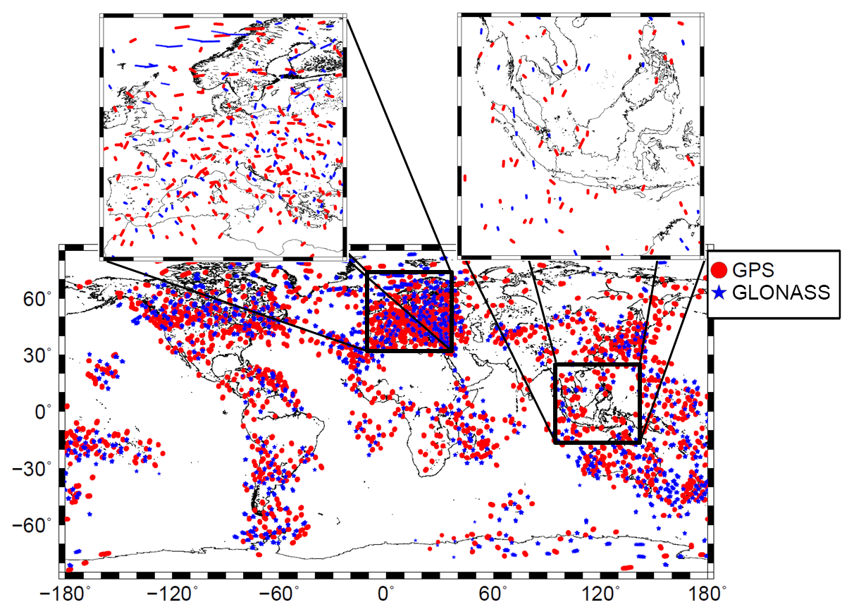
Figure 1Global distribution of the IPPs from GPS (red dots) and GLONASS (blue stars) measurements for 6 September 2017 collected within a 10 min interval between 12:55 and 13:05 UT. The regional maps at the top are “zoom-ins” of Europe and Indonesia.
By increasing the temporal resolution of the GIMs, the number of observations supporting the individual maps decreases. The two “zoom-in” maps at the top of Fig. 1 show the strong incongruity between the data distribution and the signal structure (cf. Fig. 9a, c). In areas with high-resolution data, such as Europe, the US or Australia, the VTEC signal is usually rather smooth. In areas with highly variable spatial and temporal signal structures such as in the equatorial belt, a much smaller number of observations is generally given. As a consequence, for global modeling we have to deal with a trade-off between signal structure and data resolution.
It is a well-known fact that SHs as global basis functions are not suitable for representing unevenly, globally distributed data. Consequently, in such cases, a series expansion in terms of localizing basis functions is more appropriate. In the following, we apply tensor products of polynomial and trigonometric B-splines as localizing 2-D basis functions. Besides the localizing features, B-splines additionally generate a multi-scale representation (MSR), also known as multi-resolution representation (MRR). The basic feature of a MSR is to split a target function into a smoothed, i.e., low-pass-filtered version, and a number of detail signals, i.e., band-pass-filtered versions via successive low-pass filtering (Mertins, 1999). Hence, a spatial MSR of VTEC adapts the model resolution to the data distribution and, thus, fulfills IGS' requirement of high-resolution VTEC modeling.
In this study, we compare global VTEC maps based on series expansions in terms of both globally defined SHs and localizing B-spline functions, including the MSR with respect to the spectral content. For this purpose, we use the SH degree as the common measure for the spectral content of a spherical signal. In detail, we study the interrelations between the SH degree, the spatial sampling intervals of the input data and the resolution levels of B-spline expansions. In addition, we discuss the influence of different temporal resolutions of the GIMs. For the estimation of the unknown series coefficients of the B-spline expansion, we use a Kalman filter (KF) procedure as explained by Erdogan et al. (2017). In order to assess the quality of the approach, we perform a dSTEC analysis (Hernández-Pajares et al., 2017).
The paper is outlined as follows: in Sect. 2 a description of VTEC modeling procedures based on both, SH and B-spline expansions are presented. In Sect. 2.3 we study the spectral resolution of global VTEC maps. Section 3 comprises a detailed description of the MSR and the estimation procedure. In Sect. 4 case studies are set up to verify the results of the previous sections numerically. Furthermore, this section provides a final assessment by means of a dSTEC validation. The final section provides conclusions and an outlook for future work.
The 3-D signal VTEC, introduced in Eqs. (4) and (5), can be modeled as series expansion
in terms of given space-dependent basis functions ϕk(x) and unknown time-dependent series coefficients ck(t). 1 Assuming that at discrete times with s∈ℕ0 and sampling interval Δt the total number of Is observations y(, ts) of VTEC at IPP position with is=1, 2, …, Is are given. Considering the measurement errors e(, ts), the observation equation follows from Eq. (7) and reads
Note, that we neglect the truncation error in the following
and omit other unknown parameters such as the satellite and receiver differential code biases (DCB) for GNSS geometry-free observations on the right-hand side of Eq. (8) (see, e.g., Erdogan et al., 2017).
In the following (Sect. 2.1 and 2.2), the SH expansion – as likely the most frequently used approach in ionosphere modeling – and the 2-D B-spline tensor product approach are described.
2.1 Spherical harmonic expansion
In the SH approach, the observation equation, Eq. (8), can be rewritten as
where the functions Yn,m(x), i.e., the SHs of degree n=0, …, nmax and order , …, n, are defined as
with being the normalized associated Legendre functions of degree n and order m. The total (nmax+1)2 quantities cn,m(t) in Eq. (10) are the time-dependent SH coefficients. According to the sampling theorem on the sphere, the maximum degree nmax is related to the sampling intervals Δφ and Δλ of the input data with respect to latitude φ and longitude λ, namely
As can be seen from Eq. (11), SHs are basis functions of global support. This implies that each single SH function is different from zero almost everywhere on the sphere ΩH. Consequently, each coefficient cn,m has to be recomputed if only one additional observation is considered in the set of observation Eq. (10).
As the VTEC observations at the IPP positions will usually not be given on a spatial grid with constant mesh size, the sampling intervals Δφ and Δλ in the formulae of Eq. (12) have to be interpreted as global average values.
2.2 B-spline expansion
At DGFI-TUM we rely on B-splines as basis functions for ionosphere modeling, as they are (1) characterized by their localizing feature and (2) they can be used to generate a MSR. For VTEC modeling we rewrite Eq. (8) as
with initially unknown time-dependent scaling coefficients and the 2-D scaling functions of levels J1 and J2 with respect to φ and λ. The latter are defined as tensor products
of the 1-D scaling functions and depending on latitude φ and longitude λ, respectively. As the B-spline approach is not as well known as the SH approach, it will be described in more detail in the following; we further refer to Dierckx (1984); Stollnitz et al. (1995a, b); Lyche and Schumaker (2001); Jekeli (2005); Schmidt (2015b) and citations therein.
To decompose VTEC into its spectral components via the MSR in Sect. 3, Eqs. (13) and (14) need to be rewritten in vector and matrix notation. For this purpose we introduce the vector
the vector
and the coefficient matrix
Considering the computation rules for the Kronecker product “⊗” (cf. Koch, 1999), Eq. (13) can be written as
where “vec” refers to the vec operator.
2.2.1 Polynomial B-splines
In the following, we apply polynomial quadratic B-splines
of resolution level J1∈ℕ0 and shift k1=0, 1, …, to represent the latitude-dependent variations of VTEC. To be more specific, a total of B-splines are located along a meridian depending on the latitude . To construct the B-spline functions, the sequence
of knot points is established; the consideration of multiple knot points at the poles is called “endpoint-interpolating” and ensures the closing of the modeling interval. The constant distance between two consecutive knots and for k1=2, …, amounts to . Following Schumaker and Traas (1991) and Stollnitz et al. (1995b) the normalized quadratic polynomial B-splines can be calculated via the recursive relation
with from the initial values
Note, in Eq. (21) a factor is set to zero if the denominator is equal to zero.
As can be seen from Fig. 2, B-splines are characterized by their compact support or – in other words – they are different from zero only within a small subinterval of length , where
refers to the approximate distance between two consecutive B-splines along the meridian. As the total number of B-splines depends on the level J1, finer structures can be modeled by increasing J1. The numerical value for the level J1 depends on the global average value Δφ for the input data sampling interval in the latitudinal direction according to
(Schmidt et al., 2011). Solving Eq. (23), considering the level value J1 from Eq. (22), the inequality
results.
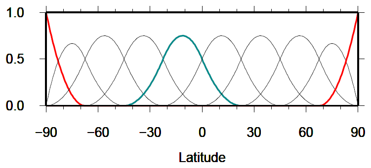
Figure 2Polynomial B-splines of level J1=3 with a total number of B-splines along the meridian. The blue spline function corresponds to the shift value k1=4 and covers a subinterval of length . The red spline functions with shift value k1=0 and with shift value k1=9 close the modeling interval at the poles.
2.2.2 Trigonometric B-splines
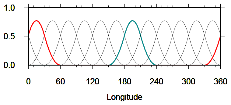
For modeling the longitudinal variations of VTEC trigonometric B-splines of order 3 and, depending on the resolution level, J2∈ℕ0 and shift k2=0, 1, …, are applied. As can be seen from Fig. 3, the total number of trigonometric B-splines are located along the parallels of the chosen spherical coordinate system within the interval . Consequently, the first and the last two B-spline functions within the interval have to be completed by the so-called “wrapping around” effect. This constraint allows trigonometric B-splines to be defined in two different ways:
-
Following Schumaker and Traas (1991), Jekeli (2005) and Limberger (2015) periodic trigonometric B-splines can be calculated by means of a recurrence relation similar to Eq. (21). Thereby, additional constraints have to be introduced to force the periodicity of the series coefficients.
-
The second option was introduced by Lyche and Schumaker (2001) and used by Schmidt et al. (2011) and Schmidt (2015b). It will be described in the following in more detail.
To be more specific, the sequence of nondecreasing knot points
with additional knots
for considering the periodicity is introduced. Similar to the polynomial B-splines, the distance between consecutive knots and for k2=0, 1, …, is given as
thus, the length of the nonzero subinterval of a trigonometric B-spline function reads . Following Lyche and Schumaker (2001) we define the functions
Setting and for the sake of simplification, the functions can be calculated via
Finally, we define the basis functions
introduced in Eq. (14). Figure 3 shows trigonometric B-splines of level J2=2. With larger values for level J2 the splines become more narrow and finer structures can be modeled. The choice of the level value J2 again depends on the input data sampling interval. Analog to Eq. (23), the inequality
has to be fulfilled, where Δλ denotes the global average value of the data sampling interval in the longitudinal direction. Finally, taking Eq. (27) into consideration, the inequality
for the level value J2 is obtained.
2.3 Spectral resolution of global VTEC models
In Sect. 2.1 we derived the relations between the maximum degree nmax of a SH expansion and the sampling intervals Δφ and Δλ of the input data. In Sect. 2.2 the corresponding relations between the level values J1 and J2 of a B-spline expansion and the data sampling intervals have been deduced. The substitution of the expression from the inequalities Eq. (12) into Eqs. (24) and (32) yields a total of six inequalities
Given the numerical values 1 to 6 for the B-spline levels J1 and J2 Table 1 presents the corresponding largest numerical values for each, the SH degree nmax and the sampling intervals Δφ and Δλ by evaluating the inequalities using Eq. (33).
Table 1Numerical values for the B-spline levels J1 and J2, the maximum SH degree nmax and the input data sampling intervals Δφ and Δλ by evaluating the inequalities from Eq. (33); the left part of the table presents the numbers along a meridian (upper inequalities in Eq. 33), and the right part represents the corresponding numbers along the Equator and its parallels according to the lower inequalities in Eq. (33).

From the spectral point of view the six inequalities from Eq. (33) comprise the following three scenarios:
-
If the global sampling intervals Δφ and Δλ are known, the mid parts of the inequalities from Eq. (33) are given. The maximum degree nmax is calculable from the right-hand side inequalities and may be inserted into the SH expansion in Eq. (10). The left-hand side inequalities yield the two level values J1 and J2 which can be inserted into the B-spline expansion from Eq. (13).
-
With a specified numerical value for nmax the right-hand parts of the inequalities from Eq. (33) are given. The data input sampling intervals Δφ and Δλ can be determined from the mid parts of the inequalities. Next, the two numerical values for the level values J1 and J2 can be calculated from the left-hand side inequalities and can be inserted into the B-spline expansion in Eq. (13).
-
If the processing time of VTEC maps has to be considered, the level values J1 and J2 are subject to certain restrictions; this is due to the fact that the number of numerical operations increases exponentially with the chosen numerical values for the levels. In this case, from the given left-hand side inequalities, the data sampling intervals Δφ and Δλ can be determined from the mid parts. Finally, the right-hand side inequalities yield numerical values for the maximum SH degree nmax.
As already mentioned in the introduction, most of the GIMs produced by the IAACs are based on series expansions in SHs up to a maximum degree of nmax=15. Following the abovementioned second strategy and Table 1, we obtain the approximations J1=4 (for nmax=17) and J2=3 (for nmax=12) for the two B-spline levels J1 and J2 for this example. Inserting these numbers into the B-spline expansion Eq. (13) yields the spectrally closest representation to the current IGS solutions. A numerical verification of this choice will be presented in Sect. 4.3.
2.4 VTEC output grids
The VTEC GIMs of the IAACs are usually provided with a spatial resolution of in the latitudinal direction and in the longitudinal direction as well as a temporal sampling of ΔT=2 h. Note, the resolution intervals ΔΦ, ΔΛ and ΔT are usually distinct from the sampling intervals Δφ, Δλ and Δt of the observations introduced in Sect. 2.1.
In order to calculate a VTEC value VTEC at an arbitrary location with and at an arbitrary time moment t, a simple bilinear spatial interpolation from the VTEC values of the four given corner points P(φi,λk), , and is performed according to
(see, e.g., Schaer et al., 1998, Fig. 4 in this paper).
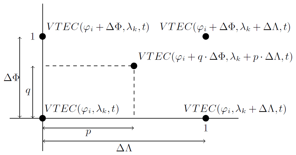
Figure 4Schematic representation of the four-point spatial interpolation to calculate the VTEC value at from the four corner points of the grid cell of interest.
Note, by applying the interpolation formula (34), the quality of the calculated VTEC value decreases with increasing spatial resolution intervals ΔΦ and ΔΛ and depends on the position within the grid cell. In order to improve the quality of the VTEC computation two methods can be used:
-
the chosen model approach, e.g., the SH or the B-spline expansion can be used directly to calculate VTEC values at any arbitrary point P(φ,λ);
-
the resolution intervals ΔΦ and ΔΛ of the output grid can be set to smaller values, e.g., to 1∘, as was proposed at the IGS workshop 2012.
For the calculation of a VTEC value VTEC at an arbitrary time moment with at a given spatial location P(φ,λ), an interpolation with respect to time can be applied. Commonly, the linear interpolation
between the two consecutive maps at epochs ts and ts+ΔT is performed (see, e.g., Schaer et al., 1998).
The previously described interpolation methods allow for the calculation of VTEC values VTEC at any spatial location P(φ,λ) and at any time t. However, for a more accurate calculation of VTEC an increase in the resolution is necessary for both domains. In the following, it is shown that the usage of a MSR based on the B-spline approach in combination with a KF estimation procedure provides the possibility to create VTEC maps of higher spatial and temporal resolution. Consequently, according to Table 1 the calculated VTEC maps cover a wider spectral band, i.e., the numerical value of nmax becomes larger.
The B-spline functions as introduced in Sect. 2.2.1 and 2.2.2 allow for the generation of a MSR. To be more specific, B-spline tensor product wavelet functions will be constructed which are intrinsically connected to the resolution levels of the MSR. Usually the MSR is interpreted as viewing a signal under different resolutions, as a microscope does (see, e.g., Schmidt, 2012; Schmidt et al., 2015a; Schmidt, 2015b; Liang, 2017). In all of the aforementioned studies, the MSR is based on a regional 2-D representation of VTEC in terms of tensor products of polynomial B-spline functions only. Within this study, however, we apply the MSR for a global 2-D representation of VTEC in terms of tensor products of polynomial and trigonometric B-spline functions, as described by Lyche and Schumaker (2001) and Schumaker and Traas (1991).
3.1 Pyramid algorithm
Neglecting the time dependency, the B-spline approach Eq. (18) reads
In the context of the MSR the vectors and are called scaling vectors, and the elements of the matrix are denoted as scaling coefficients.
With and we obtain the 2-D MSR of the target function f(x) introduced in Eq. (7) as
Following the argumentation of Schmidt et al. (2015a) but considering the polynomial and the trigonometric B-spline functions the low-passed-filtered level signal and the band-pass-filtered level detail signals can be computed via the following relations:
where we introduced the definitions and for . Herein, the and scaling vectors and as well as the and wavelet vectors and can be calculated by means of the two-scale relations
with and .
The numerical entries of the matrix and the matrix can be taken from Stollnitz et al. (1995b) or Zeilhofer (2008); the corresponding entries of the matrix and the matrix are provided by Lyche and Schumaker (2001).
In Eq. (38) we introduced the matrix of scaling coefficients as well as the matrix , the matrix and the matrix of wavelet coefficients. These four matrices can be calculated via the 2-D downsampling equation
also known as the 2-D pyramid algorithm. The matrix , the matrix , the matrix and the matrix can be computed via the identities
(see, e.g., Schmidt, 2007). The 2-D pyramid algorithm based on the decomposition Eq. (37) is visualized in Fig. 5. The “zeroth” step transforms the observations according to Eqs. (13) and (18) into the elements of the scaling matrix as introduced in Eq. (17). The procedure applied will be explained in Sect. 3.2.

The previously described MSR refers to a successive low-pass filtering of the target function into two directions, namely latitude φ and longitude λ, in the same manner. If a signal is represented according to Eq. (18) up to the level values J1 with respect to latitude and J2 with respect to longitude, i.e., , the application of the MSR Eq. (37) allows for the computation of low-pass-filtered signal approximations up to the level pairs , ,… . The principal structures of the ionospheric key parameters such as VTEC, however, are usually parallel to the geomagnetic Equator. Consequently, we will additionally deal with a 1-D MSR of the signal with respect to the latitude. In this case Eq. (37) reduces to
Thus, signal approximations up to the level pairs , , … are obtained. From the four relations in Eq. (38) only the first and the third one have to be considered within the 1-D MSR Eq. (43), namely
with for , and . The matrix of scaling coefficients and the matrix of wavelet coefficients can be calculated from the 1-D downsampling equation
where the matrices and can be computed via Eq. (41). The 1-D pyramid algorithm based on the decomposition Eq. (43) is visualized in Fig. 6.
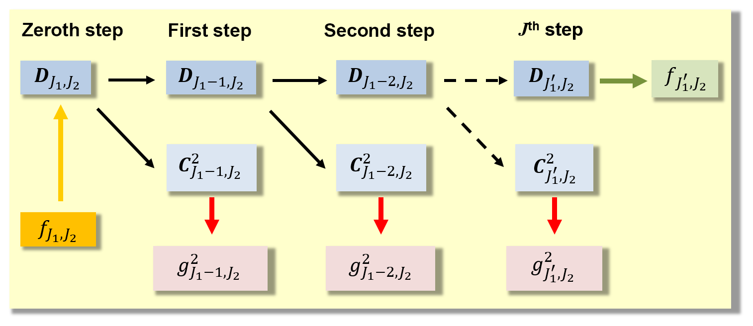
Figure 6A 1-D MSR of the signal with respect to the latitude φ. The “zeroth” step on the left-hand side conforms with the one in Fig. 5.
Besides the representation of a signal, e.g., VTEC, by means of approximations on different resolution levels with respect to latitude and longitude, the MSR also allows for the utilization of a powerful “data compression procedure”, as the numerical value of a large number of wavelet coefficients is generally close to zero depending on the signal structure (see, e.g., Zeilhofer, 2008).
3.2 Estimation of unknown model parameters
To estimate the elements of the unknown matrix from VTEC observations (cf. Eq. 8) within the “zeroth” step of the MSR we apply Kalman filtering according to Erdogan et al. (2017).
In the linear formulation the Kalman filter consists (1) of the state equation
and (2) of the system
of observation equations. In Eq. (46 ) the u×1 vector – known as the state vector – of the unknown scaling coefficients at time moment ts is predicted from the state vector βs−1 of the previous time moment ts−1 by means of the u×u transition matrix Fs and the u×1 vector ws−1 of the process noise. In Eq. (47) and are the Is×1 vectors of the observations and the measurement errors, respectively; the (is)th row vector of the Is×u coefficient matrix As is given by the expression
as introduced in Eq. (18). The measurement error vector es and the vector ws of the process noise are assumed to be white noise vectors with expectation values E(es)=0 and E(ws)=0, and fulfill the requirements
where δs,l is the delta symbol that equals 1 for s=l and 0 for s≠l. In Eq. (49) Σy and Σw are given covariance matrices of the observations and the process noise, respectively.
The solution of the estimation problem as defined in Eqs. (46) and (47) generally consists of the sequential application of a prediction step (time update) and a correction step (measurement update). In the prediction step, the estimated state vector and its covariance matrix are propagated from the time moment ts−1 to the next time moment ts by means of
where the symbol “–” indicates the predicted quantities. The prediction step is followed by the measurement update
where and are the updated state vector and its covariance matrix, respectively. In Eqs. (52) and (53) the u×Is Kalman gain matrix
behaves as a weighting factor between the new measurements and the predicted state vector. The chosen step size within the KF determines the maximum temporal resolution of the output.
Using the estimations and from Eqs. (52) and (53), a V×1 vector fs of function values at arbitrary locations P(φi,λk) with i=1, …, I, k=1, …, K and can be estimated by
where is the estimated V×V covariance matrix of the estimation . The V×u matrix is set up in a similar way to matrix As in Eq. (47) with Eq. (48). In the following, we will interpret the function values as VTEC values.
3.3 B-Spline model output
The previously explained procedure allows for the dissemination of two products to the users:
-
Product 1: a set of estimated scaling coefficients
from Eq. (52) at time moments ts for level values J1 and J2 at the spatial positions k1 in the latitudinal direction and k2 in the longitudinal direction, respectively, as well as their estimated standard deviations
extracted from the covariance matrix Eq. (53).
-
Product 2: estimated VTEC values given as
according to Eq. (55) at time moments ts for level values J1 and J2 in the latitudinal and longitudinal direction, respectively, calculated at grid points P(φi,λk) as well as their estimated standard deviations
extracted from the covariance matrix Eq. (56).
According to Eq. (35), the time interval ΔT between two consecutive maps of the coefficients Eq. (57) and their standard deviations Eq. (58) or the VTEC grid values Eq. (59) and their standard deviations Eq. (60) at times ts and ts+ΔT can be chosen arbitrarily, e.g., as 10 or 15 min, 1 h or 2 h. Following Eq. (34), the coordinates φi and λk of all of the V grid points P(φi,λk) are defined as with and with . As previously mentioned, the spatial resolution intervals ΔΦ and ΔΛ are usually chosen as 1∘, 2.5∘ or 5∘, i.e., I=181, 73, 37 and K=360, 144, 72.
The two products, i.e., the set of coefficients or the VTEC grid values reflect the two strategies of dissemination. In case of a SH expansion for RT applications as introduced in Sect. 2.1 the corresponding SH coefficients cn,m from Eq. (10) can be transferred to the user by means of a RTCM (Radio Technical Commission for Maritime services) standard 1264 message. This message allows for the consideration of SH coefficients, but only up to degree n=16. In the case of the B-spline expansion Eq. (13), however, an encoder procedure for the B-spline coefficients Eq. (57) is necessary, because the user has to evaluate the B-spline model just as in the SH case by substituting the B-spline tensor product Eq. (14) for the SHs Eq. (11). Due to the two restrictions, namely the sole use SH expansions and only up to a maximum degree nmax=16, the RTCM message format for data dissemination has to be urgently discussed and must be set up in a more flexible way (refer to the comments in Sect. 5). To apply the RTCM format in its current form, the VTEC grid values Eq. (59) can alternatively be used as observations in Eq. (10) to calculate SH coefficients cn,m(ts) by means of a least-squares estimation. This way each GIM can be sent at a high update rate to the user for RT applications.
For Product 2, the VTEC grid values Eq. (59) as well as there standard deviations Eq. (60) are disseminated as VTEC and standard deviation maps, i.e., GIMs, with given spatial resolutions ΔΦ and ΔΛ in the latitudinal and longitudinal direction, respectively, in IONEX format to the user.
In the following, the described modeling approach developed at DGFI-TUM is applied to real data. To be more specific, we use GPS and GLONASS NRT data in hourly blocks and apply ultra-rapid orbits. A detailed explanation of the data preprocessing and the setup of the full observation equations is presented by Erdogan et al. (2017). The IGS IAACs provide final products based on post-processed GNSS observations and orbits with a latency of more than 1 week. Several IAACs additionally provide rapid products with a latency of 1 d using rapid orbits. An overview on the products used in the this paper is given in Table 2.
Table 2List of GIM products used in this paper. Information on names, types and latencies are taken from the following references: (1) Roma-Dollase et al. (2017), (2) Orus et al. (2005) and (3) this paper.

For the evaluation of the data we have to define an appropriate coordinate system. Here we follow the standard procedure and use a sun-fixed geomagnetic coordinate system. To be more specific, we identify the coordinate system ΣE introduced in the context of Eq. (3) with the Geocentric Solar Magnetic (GSM) coordinate system (see, e.g., Laundal and Richmond, 2017). Consequently, the SH and B-spline theory as presented in the previous sections is applied in the orthogonal GSM system. As diurnal variations of the ionosphere are mitigated in this coordinate system, the transition matrix Fs introduced in the state Eq. (46) of the KF can be set to the identity matrix I, i.e., Fs=I. In other words, the dynamic system of the KF is set to a random walk process. Furthermore, for the time update in Eq. (46) we fix the step size to 5 min.
While the scaling coefficients Eq. (57) and their standard deviations Eq. (58) of Product 1 are located within the GSM system, the VTEC values Eq. (59) and their standard deviations Eq. (60) of Product 2 are provided in the aforementioned IONEX format on a regular grid defined in a geographical geocentric Earth-fixed coordinate system. Thus, a coordinate system transformation has to be interposed.
4.1 Validation procedure
For validation purposes we rely on the dSTEC analysis which is currently regarded as the standard method for the quality assessment of VTEC models (see, e.g., Orus et al., 2007; Rovira-Garcia et al., 2015).
This analysis method is based on the calculation of the difference between STEC observations STEC at discrete time moments ts according to Eq. (2) and a reference observation STEC along a specified satellite arc as
The reference time moment t=tref is usually referred to the observation with the smallest zenith angle z=zref. In the same manner, the differences
are calculated by means of Eq. (5) from the VTEC map to be validated. The quality assessment is performed by studying the differences
with expectation value E(dSTEC(ts))=0.
4.2 Estimation of B-spline multi-scale products
Figure 7 shows the global distribution of the IPPs related to GNSS VTEC observations as introduced in Eq. (13) for 6 September 2017 at 13:00 UT. As the B-spline model is set up in the GSM coordinate system and the scaling coefficients are restricted to the state equation
according to Eq. (46), we select and as appropriate values for the global average sampling interval of the input data as introduced at the end of Sect. 2.1. Consequently, the B-spline levels to J1=5 and J2=3 are taken from Table 1.
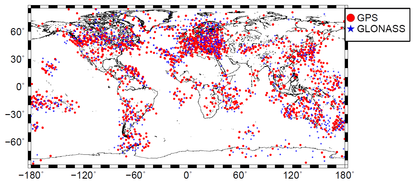
Figure 7Global distribution of the IPPs from GPS (red dots) and GLONASS (blue stars) measurements for 6 September 2017, at 13:00 UT.
The covariance matrices Σy and Σw of the observations and the process noise, respectively, as defined in the formulae of Eq.(49), are set up according to Erdogan et al. (2017). In more detail, Σy consists of two diagonal block matrices related to GPS and GLONASS VTEC observations. The relative weighting between the blocks, i.e., between GPS and GLONASS, is performed by manually defined variance factors.
Figure 8a shows with , and , the numerical values of the total scaling coefficients are
according to Eq. (57), estimated by means of Eq. (52). As the shift values k1 and k2 determine the location of the scaling coefficients, they can be plotted. Figure 8b shows the corresponding standard deviations as defined in Eq. (58). A test of significance is performed for each of the scaling coefficients according to Koch (1999).
While Fig. 8a and b show the results of Product 1 in the GSM system, Fig. 8c and d depict the corresponding results of Product 2 in a geographical geocentric coordinate system. With the choices and for the grid spacing in the latitudinal and longitudinal directions, respectively, Product 2 provides the VTEC grid values
and the corresponding standard deviations from Eqs. (59) and (60).

Figure 8Estimated scaling coefficients (a) and their standard deviations (b) for level values J1=5 and J2=3 within the GSM coordinate system. Estimated VTEC values (c) and their standard deviations (d) as GIMs within a geographical coordinate system; all sets calculated for 6 September 2017 at 13:00 UT.
Note that for the visualization of VTEC and their standard deviations in Fig. 8c and d, we computed function values on a much denser grid using the interpolation formula (34).
From the comparison of Fig. 8a and c, it can be stated that the numerical values of the scaling coefficients directly reflect the signal structure, i.e., the signal energy. This fact is the consequence of the localizing character of the B-spline functions. Figure 8b and d reveal that the standard deviations are generally larger where no or only a few GNSS observations from IGS stations are available, namely over the oceans, e.g., the Southern Atlantic, but also over specific continental regions such as the Sahara and the Amazon region.
Figure 8a, i.e., the plot of the set of scaling coefficients in Eq. (65) can be interpreted as a visualization of the 34×24 matrix D5,3 defined in Eq. (17) and displayed in the top-left boxes of Figs. 5 and 6 for the 2-D and the 1-D MSR, respectively. Consequently, Fig. 8a and b are the results of the zeroth step within the pyramid algorithm, as explained in Sect. 3. Applying the first step of the 1-D pyramid algorithm, the downsampling Eq. (44) provides both the 18×24 matrix D4,3 of estimated scaling coefficients for the level values J1=4 and J2=3 as well as the 16×24 matrix of estimated wavelet coefficients. Consequently, the definition of Product 2 in Sect. 3.3 can be extended to “Multi-Scale Products 2”:
-
ophg: estimations with levels J1=5, J2=3
-
oplg: estimations with levels J1=4, J2=3
We denote the two Multi-Scale Products 2 as “ophg” and “oplg”', where the first symbols refer to the OPTIMAP processing software, which was developed within a third-party funded project (see Acknowledgements). The “p” is chosen according to the temporal output sampling ΔT of maps, with “t” for ΔT=10 min, “1” for ΔT=1 h and “2” for ΔT=2 h. The third symbol describes the spectral resolution and is selected as “l” for “low” and “h” for “high”. Finally, the last symbols indicates the model domain and is set to “g” for “global”. Furthermore, we want to mention again, that the “ophg” and “oplg” products are all presented in geographical coordinates.
4.3 Comparison of VTEC maps from B-spline and spherical harmonic expansions
As mentioned in the context of Table 1, the B-spline levels J1=4 for latitude and J2=3 for longitude fit best to the highest degree nmax=15 of a SH expansion Eq. (10). To be more specific, we compare the multi-scale product “o1lg” with the product “codg” provided by CODE. “codg” is characterized by a SH expansion up to degree nmax=15 and a time interval ΔT=1 h of two consecutive maps (Schaer, 1999).
Figure 9 shows the VTEC and standard deviation maps for 6 September 2017 at 13:00 UT as well as the difference map between “o1lg” and “codg”. Although the structures of the two VTEC maps are rather similar, the difference map shows deviations of up to ±6 TECU. To judge this amount, a comparison of VTEC GIMs from different IAACs was performed (not shown here). This investigation stated that deviations between individual IAAC products can reach ±10 % or even more. Studying the structures within the difference map no larger systematic patterns are visible and, thus, justify our assumption that the quality of “o1lg” is comparable with the quality of the IAAC products. The standard deviation maps in Fig. 9b and d show different structures that are mainly caused by the application of the different estimation strategies, namely KF (“o1lg”) and least-squares estimation (“codg”).
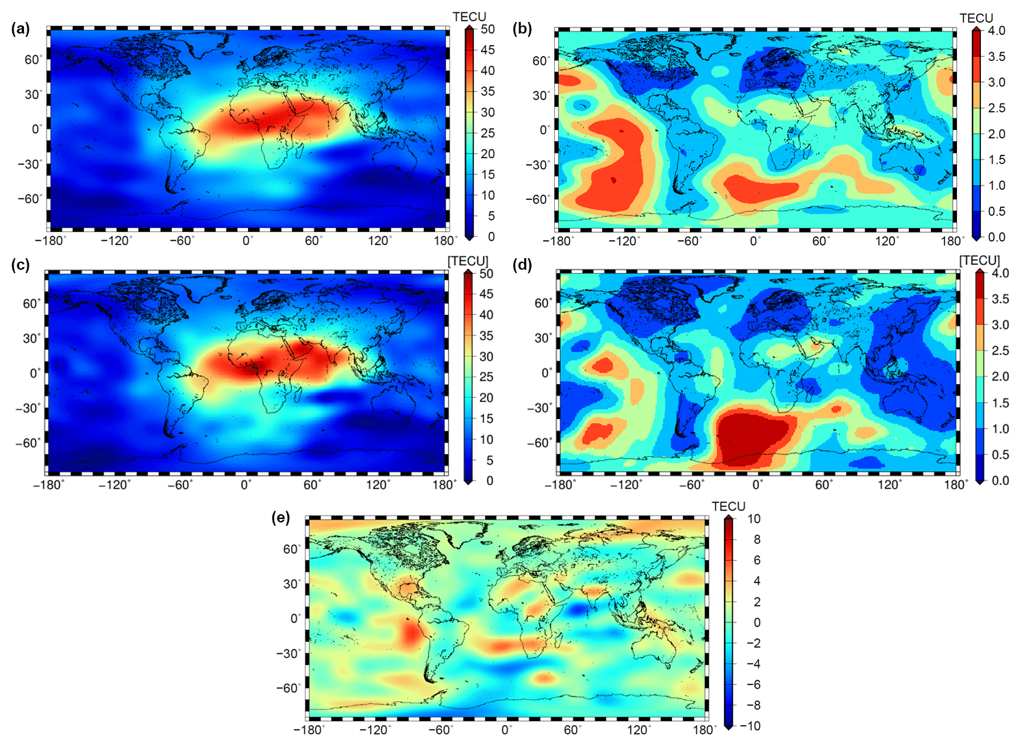
Figure 9VTEC maps “codg” (a) and “o1lg” (c) as well as their standard deviation maps (b, d); difference map of the two VTEC maps (e); all data for 6 September 2017 at 13:00 UT.
To numerically assess the comparability we apply the dSTEC analysis described in Sect. 4.1. First we define a network of receiver stations which are used in Eq. (61).
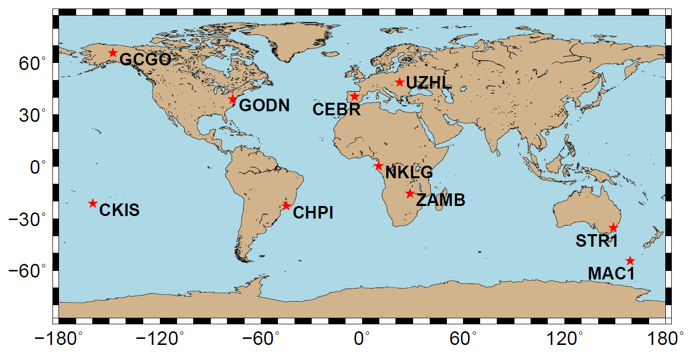
Figure 10Distribution of the 10 IGS receiver stations used for the dSTEC analysis.
The chosen set should not be used within the computation of the VTEC maps. Fulfilling both requirements at the same time is difficult and, thus, the set of stations shown in Fig. 10 contains both independent stations and stations used simultaneously in all VTEC models. As GNSS measurements are taken along the satellite arcs, the corresponding IPPs are located spatially within a grid cell and temporally between the discrete time moments of the “o1lg” and “codg” products. In order to calculate the VTEC values in Eq. (62), the spatial and temporal interpolation formulae (34) and (35) have to be applied. Figure 11 shows the RMS values of the differences Eq. (63) during the time span between 1 and 30 September 2017, at the chosen receiver stations.
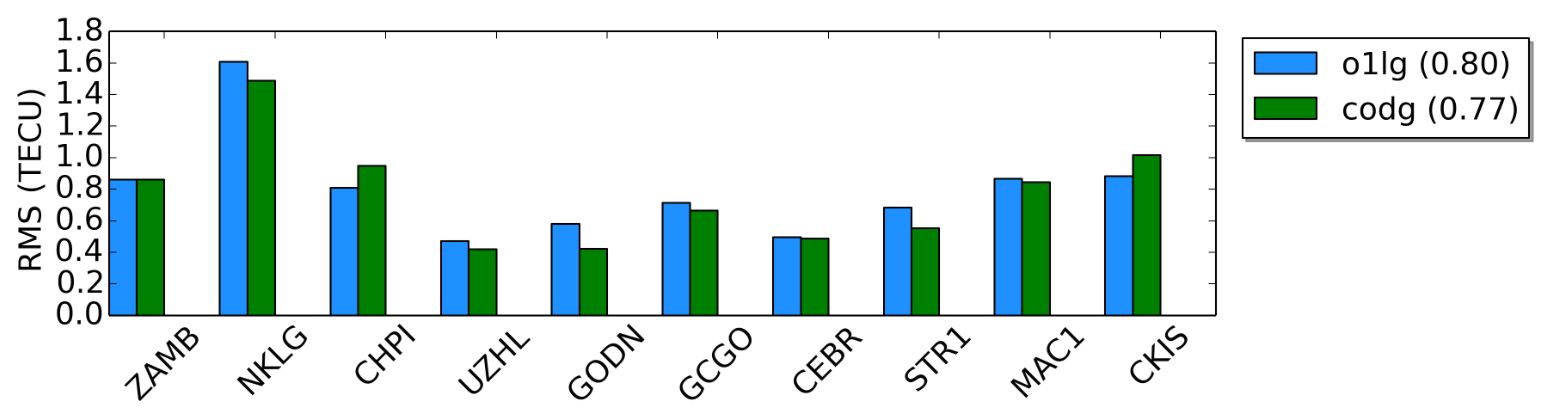
Figure 11RMS values for the “codg” (green) and “o1lg” (blue) products computed at the 10 receiver stations shown in Fig. 10. The values in parentheses in the legend are the average RMS values over all 10 receiver stations for the entire test period between 1 and 30 September 2017.
As can be seen, the RMS values vary between 0.3 and 1.6 TECU. By comparing the RMS values of “o1lg” with a mean RMS value of 0.80 TECU and “codg” with a mean RMS of 0.77 TECU we can state that the quality of these two products is very close to each other.
The results indicate that the overall quality of the NRT product “o1lg” is comparable with that of the final product “codg” including the developed and implemented preprocessing strategies and steps of the GNSS data (see Table 2).
4.4 Assessment of the multi-scale VTEC products
The two multi-scale VTEC products “ophg” and “oplg” have been introduced in the two equation blocks Eqs. (67) and (68). In what follows, we study them during a solar storm of medium intensity on 8 September 2017 and during the strongest storm of the last 10 years, the prominent St. Patrick storm, which occurred on 17 March 2015. Figure 12a, c, and d show the results of the 8 September 2017 event at 19:00 UT and Fig. 12b, d, and e display the corresponding maps for the St. Patrick storm event on 17 March 2015 at 19:00 UT.

Figure 12Multi-scale VTEC products for solar storm events: high-resolution VTEC map “ophg” for 8 September 2017 (a) and for 17 March 2015 (b); low-resolution VTEC map “oplg” for 8 September 2017 (c) and for 17 March 2015 (d); panels (e) and (f) show the detail signals introduced in equation block Eq. (68) and computed by means of Eq. (44) for the two solar events.
As already mentioned in the context of Eq. (43), it is expected that the detail signal Eq. (44) is dominated by structures parallel to the geomagnetic Equator. The detail signal shown in Fig. 12e and f meets these expectations. Especially during the St. Patrick storm event, the detail signal shows strong signatures. It should be mentioned that a large number of estimated wavelet coefficients collected in the matrix are characterized by absolute values smaller than a given threshold. The neglect of these coefficients allows for a high data compression rate. Consequently, the number of significant coefficients as the outcome of a MSR would go drastically below the number of scaling coefficients within the set Eq. (57) of Product 1; the reader can get an impression of the number of neglected coefficients by paying attention to the light green and light blue colors in Fig. 12e and f. This advantageous feature of the MSR was not studied within this work but will be applied and published in the future.
Next, we focus on the solar storm during September 2017 and study the temporal sampling intervals of different GIMs. In summary, we distinguish between six products of different spectral content and different sampling intervals.
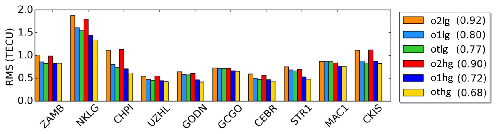
Figure 13RMS values for the “o2hg”, “o1hg”, “othg”, “o2lg”, “o1lg” and “otlg” products computed at the 10 receiver stations shown in Fig. 10 during September 2017. The values in parentheses in the legend are the average RMS values over all 10 receiver stations for the entire test period between 1 and 30 September 2017.
Figure 13 depicts the RMS values computed by the dSTEC analysis at the stations shown in Fig. 10. It is assumed that a product with a larger sampling interval ΔT is less accurate than a product with a smaller sampling interval. Consequently, the average RMS values of “o2hg” and “o2lg” are larger than the corresponding values for a shorter sampling interval. Furthermore, it is assumed that RMS values for a product with higher B-spline levels, e.g., “othg”, are smaller than for the corresponding product with lower B-spline level values such as “otlg”. By comparing the corresponding color bars in Fig. 13, i.e., orange (“o2lg”) vs. red (“o2hg”), light blue (“o1lg”) vs. blue (“o1hg”) and green (“otlg”) vs. yellow (“othg”), the aforementioned assumptions are confirmed.
The differences in the RMS values of the first three products, “o2lg”, “o1lg” and “otlg”, are caused by their different sampling intervals. Comparing the mean RMS values of 0.92 and 0.80 TECU for “o2lg” and “o1lg”, respectively, we find a relative improvement of approximately 13.0 %. By decreasing the sampling from ΔT=2 h to ΔT=10 min, a further improvement of 16.3 % can be achieved.
Table 3Relative improvements (in percentage) for a downsizing of the sampling interval of the “o2lg”, “o1lg”, “otlg”, “o2hg”, “o1hg” and “otlg” products.
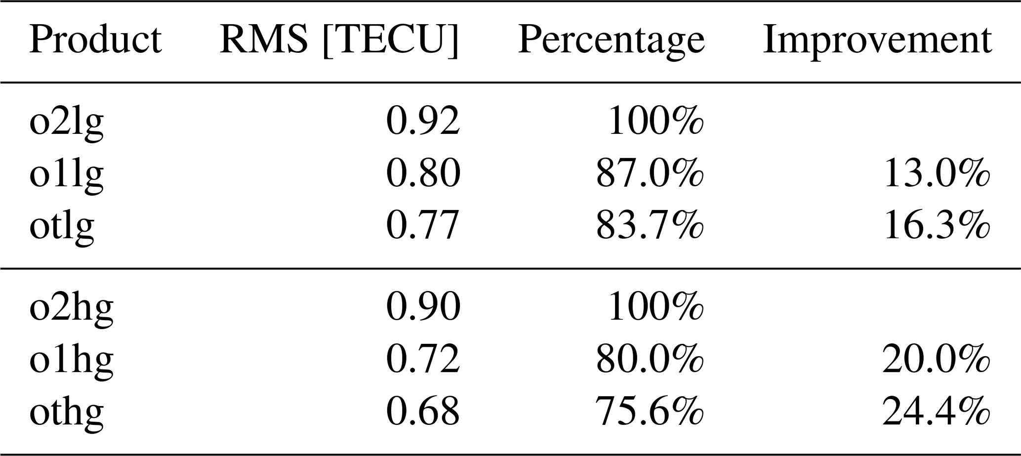
Comparing the RMS values 0.90, 0.72 and 0.68 TECU of the “o2hg”, “o1hg” and “othg” products, respectively, we find relative improvements of 20 % and 24.4 % by downsizing the sampling interval from 2 to 1 h and finally to 10 min. A summary of the relative improvements is given in Table 3.
In the next step, we compare the quality of the multi-scale products “ophg” and “oplg” directly. First, we compare “o2lg” with “o2hg” and obtain an improvement of approximately 2.2 % . In the same manner, we compare “o1lg” with “o1hg” and “otlg” with “othg” and find that improvements of 10.0 % and 11.7 % can be achieved, respectively. Table 4 shows the results for the comparison of each pair of products; an improvement is indicated by numbers in bold font, and a deterioration is indicated by numbers in italic font. As a consequence, an increase of the numerical value for level J1, i.e., the enhancement of the spectral resolution with respect to the latitude yields a significant improvement in the RMS values as long as the temporal sampling ΔT is less than 2 h.
Table 4Results (in percentage) of the comparisons of the high-resolution products “ophg” with the low-resolution products “oplg”. Positive (bold) numbers mean an improvement, and negative (italic) values represent a reduction in the quality.
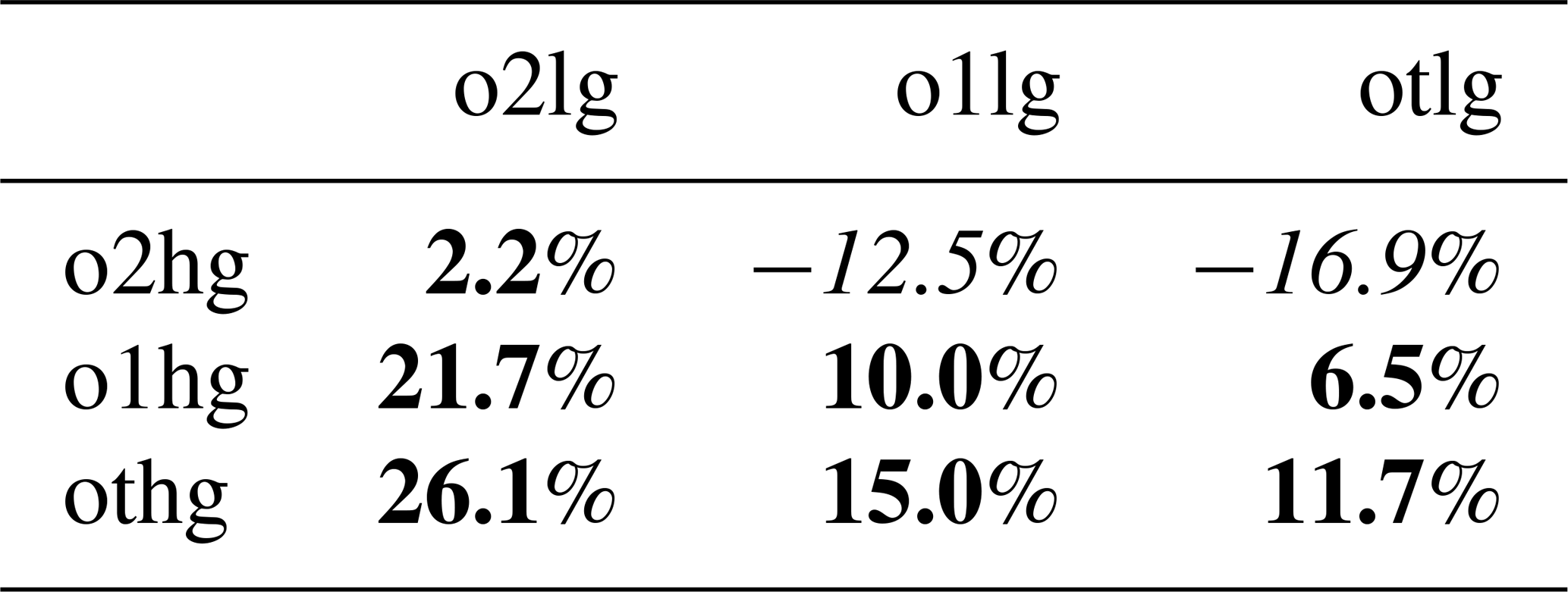
From the investigations in Sect. 4.3, it could be concluded that the quality of the “o2lg” product is comparable to the quality of the IAAC products. It can be seen from Table 4 that there is a strong improvement of more than 26 % when using the “othg” product instead of the “o2lg” product. It is worth mentioning that both products are based on the same input data and are spatially related to each other by means of the MSR.
4.5 Assessment of high-resolution VTEC models
As the “othg” product outperforms all other products used in the previous sections we now compare it with UPC's “uqrg” product (Roma-Dollase et al., 2017) which provides smaller values in the relative standard deviation of their dSTEC analysis in comparison with the products of other IAACs. “uqrg” is a rapid product and is provided with a sampling interval ΔT=15 min. As the “NKLG” station is not used in the calculation of “uqrg”, it is excluded from the calculation of the overall RMS value shown in the legend.
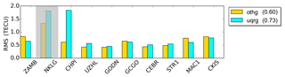
Figure 14RMS values for the “uqrg” and “othg” products computed at 9 IGS receiver stations during September 2017. The values in parentheses in the legend are the average RMS values over all 9 receiver stations for the entire test period between 1 and 30 September 2017.
As can be seen, the RMS values vary between 0.5 and 1.8 TECU but are mostly below 1.0 TECU. The dominant RMS value of “uqrg” at the “CHPI” station reduces its quality significantly. If “CHPI” is neglected, the mean RMS value of “uqrg” decrease to 0.59 TECU. Summarizing these investigations, we can state that the overall quality of the two products is very similar. Considering the fact that “othg” is a NRT product with a latency of less than 3 h, it also outperforms “uqrg” which is a rapid product with a latency of around 1 d (see Table 2). However, for a final assessment, further validation studies have to be performed between the different products.
This paper presents an approach to model VTEC solely from NRT GNSS observations by generating a MSR based on B-splines; the unknown model parameters are estimated by means of an KF. Based on this approach, a number of products have been created which differ both in their spectral content and in their temporal resolution. From our investigations we state that the MSR provides B-spline models comparable to the standard GIMs of the IAACs, mostly based on SH expansions up to degree nmax=15. As the core of the numerical study we compare our results with the most prominent VTEC maps of the IAACs to rate the quality. As the dSTEC analysis is the most frequently used validation method, we abandon a comparison with satellite altimetry products here. To summarize the validation studies, it can be stated that the high-resolution “othg” product outperforms all products used within the selected time span of investigation.
Besides the facts, that our models can handle data gaps due to the utilization of localizing basis functions, the application of a KF to include a dynamic prediction procedure and the use of the MSR to create products of different spectral content at the same time, it should be mentioned that DGFI-TUM's products
-
are based on NRT GNSS observations only, i.e., are using input data with a latency of less then 3 h (in contrast, “codg” relies on post-processed data with a latency of larger than 3 weeks, and “uqrg” relies on rapid data with a latency of at least 1 d; cf. Table 2);
-
rely on specially developed software modules (cf. Fig. 15), e.g., the preprocessing module using ultra-rapid orbits;
-
and can be disseminated to users with a delay of 2–3 h.
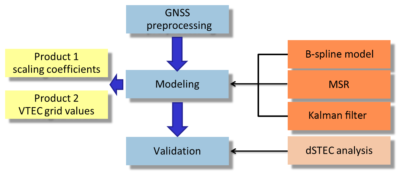
Figure 15DGFI-TUM's processing modules, including (blue boxes) the download and preprocessing module for GNSS observations, the modeling module by means of B-splines, MSR and Kalman filtering (orange boxes) with possible output as Product 1 and Product 2 (yellow boxes) and the validation module.
In general, the dissemination of these products to users can be undertaken in two different ways: based on estimated scaling coefficients (Product 1) or by calculated VTEC grid values (Product 2). For RT applications, however, the dissemination in terms of Product 1 is preferred, in particular the usage of the RTCM format. In the scope of the developments in the recent years, RT applications have become more important, e.g., in unmanned or autonomous vehicle development; thus, the restriction of the RTCM message to allow only for SH coefficients needs to urgently be discussed. Particularly from the point of view that there are also other modeling methods, a modification of the RTCM format would be appropriate. The MSR allows for significant data compression to be obtained due the step-wise downsampling of the scaling coefficients according to the pyramid algorithm. Details represented in the signal of the zeroth step are stored in wavelet coefficients for the following steps (see Fig. 5). A large number of estimated wavelet coefficients are characterized by absolute values smaller than a given threshold and, thus, most of them can be neglected for the reconstruction of the original signal. Hence, the overall number of scaling and wavelet coefficients can be reduced drastically. Considering this powerful feature of data compression, we propose replacing the scaling coefficients of the highest levels with the significant wavelet coefficients of the lower levels for a definition of an alternative and more appropriate format for data dissemination in terms of Product 1.
The results presented encourage the further development of high accuracy VTEC maps. By extending the models by a fourth dimension, i.e., modeling of the electron density directly, inaccuracies due to the mapping function can be avoided. To model the vertical structure of the electron density, additional observations have to be incorporated, e.g., from DORIS, satellite altimetry and ionospheric radio occultations. This would mitigate the inhomogeneity of the data distribution and, in turn, even higher levels of the B-spline expansion can be chosen.
The global VTEC maps in IONEX format used in the comparisons were acquired from the Crustal Dynamics Data Information System (CDDIS) data center by the following FTP server: ftp://cddis.gsfc.nasa.gov/gnss/products/ionex/. The hourly available GNSS data from IGS sites were operationally downloaded in real time through mirroring to the different IGS data centers, i.e., the CDDIS (ftp://cddis.gsfc.nasa.gov/pub/gps/data/hourly/), the Bundesamt für Kartographie und Geodäsie (BKG) (ftp://igs.bkg.bund.de/IGS/nrt/), the Institut Geographique National (IGN) (ftp://igs.ensg.ign.fr/pub/igs/data/hourly) and the Korean Astronomy and Space Science Institute (KASI) (ftp://nfs.kasi.re.kr/). Furthermore, the ultrarapid orbits of GPS and GLONASS satellites utilized in the data preprocessing step can be accessed through FTP servers: for GPS via ftp://cddis.gsfc.nasa.gov/pub/gps/products, and for GLONASS via ftp://ftp.glonass-iac.ru/MCC/PRODUCTS/.
The concept for the paper was proposed by AG and discussed with all co-authors. AG compiled the figures and wrote the paper with assistance from MS. The paper and figures were reviewed by all co-authors.
The authors declare that they have no conflict of interest.
We are grateful to the Bundeswehr GeoInformation Centre (BGIC) and the German Space Situational Awareness Centre (GSSAC) for funding the “Operational tool for ionosphere mapping and prediction” (OPTIMAP) project. The approach presented was developed within this framework.
The authors express their thanks to the following services and institutions for providing the input data: IGS and its data centers, the Center for Orbit Determination in Europe (CODE, Berne, Switzerland) and the Universitat Politècnica de Catalunya/IonSAT (UPC, Barcelona, Spain). Furthermore, the authors acknowledge the developers of the Generic Mapping Tools (GMT) which was primarily used for generating the figures in this work.
This work was supported by the German Research Foundation (DFG) and the Technical University of Munich (TUM) in the framework of the Open Access Publishing Program.
This paper was edited by Dalia Buresova and reviewed by Ilya Edemskiy and one anonymous referee.
Bassiri, S. and Hajj, G.: High-order ionospheric effects on the global positioning system observables and means of modeling them, Manuscr Geodetica, 18, 280–289, 1993. a
Bundesamt für Kartographie und Geodäsie, available at: ftp://igs.bkg.bund.de/IGS/nrt/TS6/, last access: 9 August 2019.
CDDIS: GNSS data, available at: ftp://cddis.gsfc.nasa.gov/pub/gps/data/hourly/TS5, last acces: 9 August 2019.
Crustal Dynamics Data Information System: The global VTEC maps in IONEX format used in the comparisons, available at: ftp://cddis.gsfc.nasa.gov/gnss/products/ionex/, last access: 9 August 2019.
Dach, R. and Jean, Y.: International GNSS Service – Technical Report 2012, Tech. Rep., available at: ftp://igs.org/pub/resource/pubs/2012_techreport.pdf (last access: 8 August 2019), 2013. a
Dettmering, D., Schmidt, M., Heinkelmann, R., and Seitz, M.: Combination of different space–geodetic observations for regional ionosphere modeling, J. Geodesy, 85, 989–998, 2011. a
Dettmering, D., Limberger, M., and Schmidt, M.: Using DORIS measurements for modeling the vertical total electron content of the Earth's ionosphere, J. Geodesy, 88, 1131–1143, https://doi.org/10.1007/s00190-014-0748-2, 2014. a
Dierckx, P.: Algorithms for smoothing data on the sphere with tensor products splines, Computing, 32, 319–342, 1984. a
Durmaz, M. and Karslioglu, M. O.: Regional vertical total electron content (VTEC) modeling together with satellite and receiver differential code biases (DCBs) using semi-parametric multivariate adaptive regression B-splines (SP-BMARS), J. Geodesy, 89, 347–360, 2015. a
Durmaz, M., Karslioglu, M. O., and Nohutcu, M.: Regional VTEC modeling with multivariate adaptive regression splines, Adv. Space Res., 46, RSOD12, https://doi.org/10.1016/j.asr.2010.02.030, 2010. a
Erdogan, E., Schmidt, M., Seitz, F., and Durmaz, M.: Near real-time estimation of ionosphere vertical total electron content from GNSS satellites using B-splines in a Kalman filter, Ann. Geophys., 35, 263–277, https://doi.org/10.5194/angeo-35-263-2017, 2017. a, b, c, d, e, f
Feltens, J. and Schaer, S.: IGS Products for the Ionosphere, Tech. Rep., european Space Operation Centre and Astronomical Institue of the University of Berne, 1–8, 1998. a
GPS, available at: ftp://cddis.gsfc.nasa.gov/pub/gps/products, last access: 9 August 2019.
GLONASS, available at: ftp://ftp.glonass-iac.ru/MCC/PRODUCTS/T, last access: 9 August 2019.
Hernández-Pajares, M., Juan, J. M., and Sanz, J.: New approaches in global ionospheric determination using ground GPS data, J. Atmos. Sol.-Terr. Phys., 61, 1237–1247, https://doi.org/10.1016/S1364-6826(99)00054-1, 1999. a
Hernández-Pajares, M., Juan, J. M., Sanz, J., Argón-Àngel, A., Garcia-Rigo, A., Salazar, D., and Escudero, M.: The ionosphere: Effects, GPS modeling and benefits for space geodetic techniques, J. Geodesy, 85, 887–907, 2011. a
Hernández-Pajares, M., Roma-Dollase, D., Krankowski, A., García-Rigo, A., and Orús-Pérez, R.: Methodology and consistency of slant and vertical assessments for ionospheric electron content models, J. Geodesy, 19, 1405–1414, 2017. a, b, c
Institut Geographique National, available at: ftp://igs.ensg.ign.fr/pub/igs/data/hourly, last access: 9 August 2019.
Jekeli, C.: Spline Representations of Functions on a Sphere for Geopotential Modeling, Tech. Rep., 475, 7–12, 2005. a, b
Korean Astronomy and Space Science Institute, available at: ftp://nfs.kasi.re.kr/, last access: 9 August 2019.
Koch, K. R.: Parameter Estimation and Hypothesis Testing in Linear Models, Springer-Verlag Berlin Heidelberg, 1999. a, b
Komjathy, A. and Langley, R.: An assessment of predicted and measured ionospheric total electron content using a regional GPS network, Proceedings of the 1996 National Technical Meeting of The Institute of Navigation, 615–624, 1996. a
Langley, R. B.: Propagation of the GPS Signals, Springer Berlin Heidelberg, Berlin, Heidelberg, 111–149, https://doi.org/10.1007/978-3-642-72011-6_3, 1998. a
Laundal, K. and Richmond, A.: Magnetic Coordinate Systems, Space Sci. Rev., 206, 27–59, 2017. a
Liang, W.: A regional physics-motivated electron density model of the ionosphere, Ph.D. thesis, Technical University of Munich, 2017. a
Limberger, M.: Ionosphere modeling from GPS radio occultations and complementary data based on B-splines, Ph.D. thesis, Technical University of Munich, 2015. a, b, c
Liu, J. Y., Chuo, Y. J., Shan, S. J., Tsai, Y. B., Chen, Y. I., Pulinets, S. A., and Yu, S. B.: Pre-earthquake ionospheric anomalies registered by continuous GPS TEC measurements, Ann. Geophys., 22, 1585–1593, https://doi.org/10.5194/angeo-22-1585-2004, 2004. a
Lyche, T. and Schumaker, L.: A multiresolution tensor spline method for fitting functions on the sphere, Siam J. Sci. Comput., 22, 724–746, 2001. a, b, c, d, e
Lyu, H., Hernández-Pajares, M., Nohutcu, M., García-Rigo, A., Zhang, H., and Liu, J.: The Barcelona ionospheric mapping function (BIMF) and its application to northern mid-latitudes, GPS Solution, 22, 724–746, 2018. a
Mertins, A.: Signal analysis: wavelets, filter banks, time-frequency transforms and applications, Wilex, Chicester, 1999. a
Monte-Moreno, E. and Hernández-Pajares, M.: Occurrence of solar flares viewed with GPS: Statistics and fractal nature, J. Geophys. Res., 119, 9216–9227, 2014. a
Orus, R., Hernándes-Pajares, M., Juan, J., and Sanz, J.: Improvement of global ionospheric VTEC maps by using kriging interpolation technique, J. Atmos. Sol.-Terr. Phys., 67, 1598–1609, 2005. a
Orus, R., Cander, L., and Hernándes-Pajares, M.: Testing regional vertical total electron content maps over Europe during 17–21 January 2005 sudden space weather event, Radio Sci., 42, RS3004, https://doi.org/10.1029/2006RS003515, 2007. a
Roma-Dollase, D., Hernández-Pajares, M., Krankowski, A., Kotulak, K., Ghoddousi-Fard, R., Yuan, Y., Li, Z., Zhang, H., Shi, C., and Wang, C.: Consistency of seven different GNSS global ionospheric mapping techniques during one solar cycle, J. Geodesy, 92, 691–706, 2017. a, b, c, d
Rovira-Garcia, A., Juan, J., Sanz, J., and Gonzalez-Casado, G.: A Worldwide Ionospheric Model for Fast Precise Point Positioning, IEEE T. Geosci. Remote Sens., 53, 4596–4604, 2015. a
Schaer, S.: Mapping and Predicting the Earth's Ionosphere Using the Global Positioning System, Ph.D. thesis, University of Berne, 1999. a, b, c, d
Schaer, S., Gurtner, W., and Feltens, J.: IONEX: The IONosphere Map EXchange Format Version 1, Tech. Rep., Astronomical Institute, University of Berne, Switzerland, 2–3, 1998. a, b
Schmidt, M.: Wavelet modelling in support of IRI, Adv. Space Res., 39, 932–940, 2007. a, b
Schmidt, M.: Towards a multi-scale representation of multi-dimensional signals, VII Hotine-Marussi Symposium on Mathematical Geodesy, 137, 119–127, https://doi.org/10.1007/978-3-642-22078-4_18, 2012. a
Schmidt, M., Dettmering, D., Mößmer, M., and Wang, Y.: Comparison of spherical harmonic and B-spline models for the vertical total electron content, Radio Sci., 46, RS0D11, https://doi.org/10.1029/2010RS004609, 2011. a, b, c
Schmidt, M., Göttl, F., and Heinkelmann, R.: Towards the combination of data sets from various observation techniques, in: The 1st International Workshop on the Quality of Geodetic Observation and Monitoring Systems (QuGOMS'11), edited by: Kutterer, H., Seitz, F., Alkhatib, H., and Schmidt, M., 140, 35–43, 2015a. a, b
Schmidt M., Dettmering D., S. F.: Using B-spline expansions for ionosphere modeling, in: Handbook of Geomathematics, 2nd Edn., edited by: Freeden, W., Nashed, M. Z., and Sonar, T., Springer, 939–983, https://doi.org/10.1007/978-3-642-54551-1_80, 2015b. a, b, c, d
Schumaker, L. and Traas, C.: Fitting scattered data on spherelike surfaces using tensor products of trigonometric and polynomial splines, Numerische Mathematik, 60, 133–144, 1991. a, b, c
Stollnitz, E., DeRose, T., and Salesin, D.: Wavelets for computer graphics: a primer, Part I, IEEE Comput. Graph., 3, 76–84, 1995a. a
Stollnitz, E., DeRose, T., and Salesin, D.: Wavelets for computer graphics: a primer, Part I and Part II, IEEE Comput. Graph., 15, 75–85, 1995b. a, b, c
Tsurutani, B., Mannucci, A., Iijima, B., Guarnieri, F., Gonzalez, W., Judge, D., Gangopadhyay, P., and Pap, J.: The extreme Halloween 2003 solar flares (and Bastille Day, 2000 Flare), ICMEs, and resultant extreme ionospheric effects: A review, Adv. Space Res., 37, 1583–1588, 2006. a
Tsurutani, B., Verkhoglyadova, O. P., Mannucci, A., Lakhina, G. S., Li, G., and Zank, G. P.: A brief review of “solar flare effects” on the ionosphere, Radio Sci., 44, RSOA17, https://doi.org/10.1029/2008RS004029, 2009. a
Wang, C., Rosen, I. G., Tsurutani, B. T., Verkhoglyadova, O. P., Meng, X., and Mannucci, A. J.: Statistical characterization of ionosphere anomalies and their relationship to space weather events, J. Space Weather Space Clim., 6, A5, https://doi.org/10.1051/swsc/2015046, 2016. a
Zeilhofer, C.: Multi-dimensional B-spline Modeling of Spatio-temporal Ionospheric Signals, Series A, 123, 2008. a, b
Zhu, F., Yun, W., Yiyan, Z., and Gao, Y.: Temporal and spatial distribution of GPS-TEC anomalies prior to the strong earthquakes, Astrophys. Space Sci., 345, 239–246, 2013. a
Note that we do not distinguish between geographical and geomagnetic spherical coordinates for latitude φ and longitude λ.