Modeling of GPS total electron content over the African low-latitude region using empirical orthogonal functions

In this paper, an empirical total electron content (TEC) model and trends in the TEC over the African low-latitude region are presented. GPS-derived TEC data from Malindi, Kenya (geographic coordinates 40.194^∘ E, 2.996^∘ S), and global ionospheric maps (GIMs) were used. We employed an empirical orthogonal function (EOF) analysis method together with least-squares regression to model the TEC. The EOF-based TEC model was validated through comparisons with GIMs, the GPS-derived TEC and the TEC derived from the International Reference Ionosphere 2016 (IRI-2016) model for selected quiet and storm conditions. The single-station EOF-based TEC model over Malindi satisfactorily reproduced the known diurnal, semiannual and annual variations in the TEC. Comparison of the EOF-based TEC model results with the TEC derived from the IRI-2016 model showed that the EOF-based model predicted the TEC over Malindi with fewer errors than the IRI-2016. For the selected storms, the EOF-based TEC model simulated the storm time TEC response over Malindi better than the IRI-2016. In the case of the regional model, the EOF-based TEC model was able to reproduce the TEC characteristics in the equatorial ionization anomaly region. The EOF-based TEC model was then used as a background for estimating TEC trends. A latitudinal dependence in the trends was observed over the African low-latitude region.

1 Introduction

The features of the low-latitude ionosphere are quite unique. During the daytime, a double-peaked ionization structure appears over the low-latitude region, a phenomenon often referred to as the equatorial ionization anomaly (EIA). The EIA is normally explained in terms of the plasma fountain theory (Martyn, 1947; Moffett, 1979). The daytime E-region eastward electric field in combination with the nearly horizontal magnetic field of Earth generate a large vertically directed E×B drift force at the dip equator that raises the plasma to higher altitudes. The raised plasma diffuses away from the geomagnetic equator under gravity and pressure gradient forces along the equipotential magnetic field lines to form ionization peaks at dip latitudes $\sim \pm \mathrm{15}$^∘ and a trough that extends over the dip equator (Appleton, 1946). Prior to the electric field turning westwards at night, it is enhanced (pre-reversal enhancement – PRE), resulting in plasma uplift into regions of low recombination. Associated with the electron density at the EIA enhancement is a density gradient instability of the Rayleigh–Taylor (RT) type which creates a spectrum of plasma irregularities that fill the post-sunset low-latitude ionosphere (Kelley, 2009). The EIA and the PRE vary with location, solar activity and season, even on daily basis. These variations make it difficult to predict the characteristics of the low-latitude ionosphere.

The state of the ionosphere is of great importance in space-based navigation systems such as the global navigation satellite systems (GNSS). The total electron content (TEC) is of particular interest to users of GNSS systems. For many practical purposes in the GPS, the desired ionospheric parameter is the TEC. This is because many of the effects on transionospheric satellite links (e.g., time delay, polarization, Faraday rotation and Doppler shift) are related to the TEC in one way or another (Kersley et al., 2004). The low-latitude ionosphere exhibits the highest values of the TEC globally. Therefore, pronounced ionospheric effects are experienced by radio signals transiting the low-latitude ionosphere. Understanding the low-latitude ionospheric dynamics in a bid to forecast its day-to-day conditions is key for advancement of space technology and the improvement of GNSS accuracy.

Ionospheric variability over the low-latitude region of Africa, based on TEC analysis, has been reported before (e.g., Adewale et al., 2011; Olwendo et al., 2012; Habarulema et al., 2013; Andima et al., 2015). From these studies, the diurnal, seasonal, disturbed and quiet-time TEC characteristics over the region have been revealed. However, these analyses made use of TEC data of either the same solar phase or the same solar cycle. Now with a relatively longer record of data in the achieves, it is imperative to extend these studies to the long-term TEC characteristics over the African low-latitude region for practical applications.

A common approach to TEC prediction is through modeling. Various TEC models (e.g., Anderson et al., 1987; Rawer and Bilitza, 1990; Reinisch et al., 2004; Lean et al., 2011; Hajra et al., 2016; Ercha et al., 2012; Chen et al., 2015) have been developed; however, many of these models are limited in geographical extent. A widely used model to describe the global TEC climatology is the International Reference Ionosphere (IRI) model (Bilitza, 1990). The IRI is an empirical model synthesized from global data sets comprised of ionosonde, radar and in situ measurements (Bilitza, 1990; Rawer and Bilitza, 1990). Averaging and smoothing applied when deriving the model coefficients may limit its accuracy in capturing peculiar features such as the TEC variability in the EIA region. Under such circumstances, regional models are superior in characterizing the background TEC.

Long term trends in ionospheric parameters are indicative of the deviation in the ionospheric parameters from their background values. Ionospheric trends are important in understanding the changes in Earth's energy balance (Elias, 2011). Various studies (e.g., Jarvis et al., 1998; Bencze, 2002, 2005; Lastovicka et al., 2006; Danilov and Mikhailov, 1999; Bremer et al., 2012) have reported on long-term trends in ionospheric parameters derived from ionosonde data. A conclusion from these studies is that trends in the F2-layer critical frequency (foF2) and F2-layer maximum electron density height (hmF2) are negative. Some studies on ionospheric trends have also revealed latitudinal dependence of these trends (Danilov and Mikhailov, 1999). Lean et al. (2011), using a database of global ionospheric maps (GIMs), reported that global TEC trends are positive and are dependent on the geomagnetic latitude. Also cases of negligible or no trends in the TEC have been observed. For instance, results obtained by Lastovicka et al. (2017) show a weak negative trend or no trend in ionospheric TEC. Despite the various studies on trends of different ionospheric parameters, those relating to TEC remain limited, hence the question on the nature of ionospheric TEC trends still needs to be answered. There is a need to investigate whether TEC has a negative (Lastovicka et al., 2017), positive (Lean et al., 2011) or no (Lastovicka, 2013) trend. The objective of this paper is therefore twofold: first to attempt to model the low-latitude TEC, and second to estimate trends in the variation of the ionospheric TEC over the African low-latitude region using actual TEC measurements by means of regional GPS receivers and data from the GIMs.

2 Data sets used

The International GNSS Service (IGS) operates a number of GPS ground-based receivers over the African low-latitude region. In this study, data were obtained from one of the IGS receivers located at Malindi, Kenya, which archived data from 1995 to date (December 2017). Prior to 2008, the IGS receiver (station code MALI) was installed at 40.19439^∘ E, 2.99591^∘ S, and was then replaced with another (station code MAL2) installed at 40.19414^∘ E, 2.99606^∘ S. These receivers had nearly the same location and therefore sampled the same geographical region of the ionosphere. We obtained the receiver independent exchange (RINEX) files from ftp://cddis.gsfc.nasa.gov/ (last access: 15 June 2018) and then extracted the TEC along the line-of-site, slant TEC (sTEC) from the RINEX files using the GPS-TEC software of Boston College (Seemala and Valladares, 2011). This software uses the thin shell mapping function to map the sTEC to be vertical to obtain the vertical TEC (vTEC) at an assumed ionospheric height of 350 km. The vTEC for the different viewing geometries for satellites with elevation angles greater than 30^∘ were averaged epoch by epoch to give a representation of the vTEC above the receiver. Due to data paucity from 1995 to 1998, only data from 1999 to 2017 were used in this study. Hourly averages of the daily TEC data were then calculated to minimize noise in the data. The hourly averages were organized into a data matrix M_d×h (day × hour) which was used to model and estimate trends in the TEC over Malindi. To study the TEC over the African low-latitude region, the TEC from the GIMs, a reliable source of ionospheric data (Hernandez-Pajares et al., 2009), was used. Though these maps have been available since 1998, for comparison purposes with the GPS data, we have used data from 1999–2017. It is worthy noting that the 2-hourly GIMs were linearly interpolated to hourly data using a similar approach as in Jee et al. (2010).

Figure 1 The first six basis functions (a) representing the diurnal variation and their coefficients (b) which show the long-term variation of TEC over MAL2. The red curves in the top left panels in (a) and (b) compare the diurnal mean TEC with the first basis vector U₁ and the solar radio flux index measured at 10.7 cm wavelength (F10.7) with coefficients C₁ of the first EOF mode, respectively. Inserted at the top of the top left panel of (b) is a magnified section of the coefficients C₁ in 2002–2003 to show the semiannual and annual variations.

3 Single-station model over Malindi

3.1 EOF decomposition of the TEC data

Empirical orthogonal function (EOF) analysis is a well-known method that dates back to the work of Pearson (1901) and has been widely used in climate (Hannachi et al., 2007) and ionospheric (Dvinskikh, 1988; Zhang et al., 2009; Liu et al., 2008) data analysis. It involves reducing the dimensionality of the data by finding a reduced set of variables (EOF modes) that explain most of the variability in the data. This allows for the original data (TEC(d,h)) to be expressed as a linear combination of a small number of basis functions as

$$\begin{array}{}\text{(1)}& {\displaystyle }\mathrm{TEC}(d,h)=\sum _{j=\mathrm{1}}^n{U}_j\left(h\right)\times C_j\left(d\right),\end{array}$$

where C_j is the coefficient of the basis vector U_j(h) with the index j running from 1 to n (the number of the retained EOF modes). We used the method of singular value decomposition (svd) to determine the EOF modes that explain most of the variability in the TEC data. The TEC data matrix M was decomposed into U and V, the left and right basis vectors respectively, and S is a matrix of singular values of M according to the equation

$$\begin{array}{}\text{(2)}& {\displaystyle }\mathbf{M}=\mathit{U}\mathbf{S}{\mathit{V}}^{\mathrm{T}}.\end{array}$$

The basis vectors of the first six EOF modes in matrix U and their corresponding coefficients obtained using Eq. (3) are shown in Fig. 1. While Table 1 shows the percentage variability in the data explained by the different EOF modes,

$$\begin{array}{}\text{(3)}& {\displaystyle }{C}_j\left(d\right)=S\times V_j^{\mathrm{T}}.\end{array}$$

Figure 1a shows that the average diurnal TEC (red curve) over Malindi has a pre-dawn minimum at about 03:00 UT, a maximum at about 11:30 UT and an enhancement from 18:00 to 20:00 UT. The maximum at 11:30 UT is possibly due to increased ionization, as the solar zenith angle is nearly zero over Malindi around this time. The post-sunset increase in the TEC from 18:00 to 20:00 UT could be due to an enhancement in the eastward electric field before its westward reversal at night. Though the physical interpretation of the basis functions are normally difficult due to their geometric nature (Hannachi et al., 2007), the high correlation between the first basis mode U₁ with the mean TEC shows that U₁ is replicating the diurnal characteristics of the ionospheric TEC over Malindi. Figure 1b shows that the semiannual and annual variations in the TEC have peaks during the equinoxes and high solar activity years respectively. These coefficients are well correlated with the solar radio flux measured at the 10.7 cm wavelength (F10.7), confirming that the main driver of ionospheric variability over Malindi is the changes in the extreme ultraviolet (EUV) radiation.

Table 1 Variance of the TEC data explained by the different EOF modes

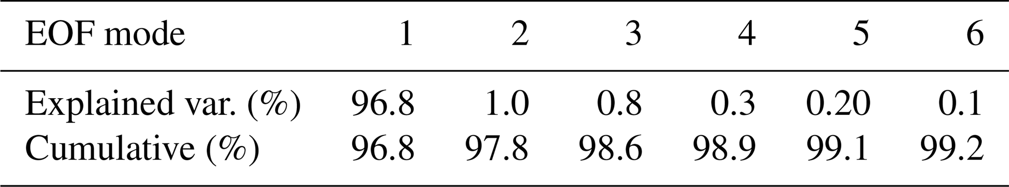
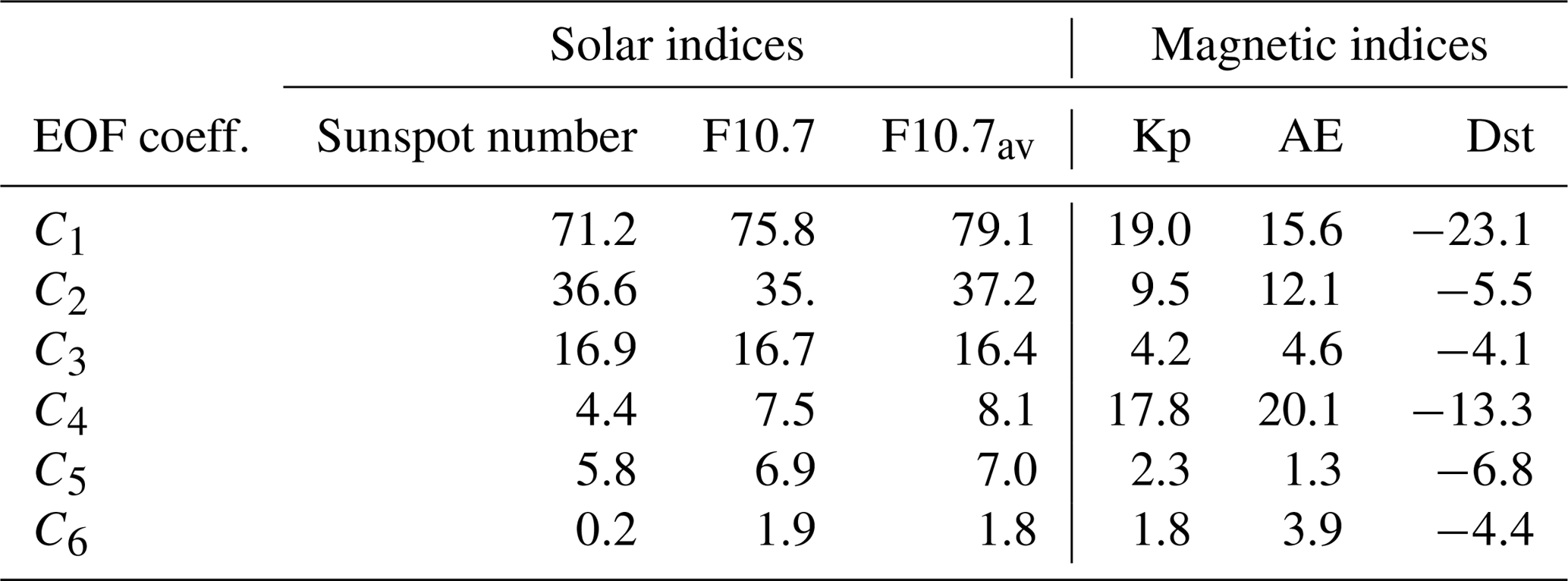
Table 2 Percentage correlation coefficients of some of the commonly used solar and magnetic indices with the first six EOF coefficients.

3.2 Modeling of the coefficients

Due to the rapid convergence of the basis functions, we used only the first six EOF modes, which accounted for 99.2 % of the explained variance in the data, to model the observed regional TEC as derived from GNSS measurements at Malindi. For an effective TEC model, the choice of the input parameters to model the solar and magnetic activity dependencies of the TEC is important. Table 2 shows the correlation coefficients expressed in percentages for some of the commonly used solar and magnetic indices obtained from Omniweb (https://omniweb.gsfc.nasa.gov/, last access: 26 December 2018) with the first six EOF coefficients. Among the solar indices, the first EOF coefficients showed a stronger correlation with the solar activity factor F10.7_av (Richards et al., 1994; Liu et al., 2006) given by $\mathrm{F}{\mathrm{10.7}}_{\mathrm{av}}=\mathrm{1}/\mathrm{2}(\mathrm{F}\mathrm{10.7}+\mathrm{F}{\mathrm{10.7}}_{\mathrm{81}})$, where F10.7₈₁ is the 81-day average of F10.7 centered on the day of interest. For the magnetic indices, the first EOF coefficients showed the highest correlation with Dst, followed by Kp and then AE. Based on the observations in Table 2, it was reasonable to use F10.7_av and Dst as inputs to model the solar and magnetic dependences of TEC over Malindi. Since Dst and F10.7_av vary with the day of the year (DOY), our third input parameter was the DOY number. We then expressed the EOF coefficients as a sum of linear and harmonic functions following the procedure of Zhang et al. (2009) as

$$\begin{array}{}\text{(4)}& {\displaystyle }{C}_j\left(d\right)=B_{j\mathrm{1}}\left(d\right)+B_{j\mathrm{2}}\left(d\right)+B_{j\mathrm{3}}\left(d\right).\end{array}$$

The term B_j1(d) accounts for the linear variation of the EOF coefficients with solar and magnetic activities and is given by

$$\begin{array}{}\text{(5)}& {\displaystyle }{B}_{j\mathrm{1}}\left(d\right)=a_{j\mathrm{1}}+b_{j\mathrm{1}}\mathrm{F}{\mathrm{10.7}}_{\mathrm{av}}\left(d\right)+c_{j\mathrm{1}}\mathrm{Dst}\left(d\right).\end{array}$$

The semiannual and annual variations in the EOF coefficients are represented in Eq. (4) by the harmonic terms B_j2(d) and B_j3(d) of periods of half a year and 1 year (365.25 days) respectively, expressed as

$$\begin{array}{ll}{\displaystyle }{B}_{j\mathrm{2}}\left(d\right)& {\displaystyle }=\left[a_{j\mathrm{2}}+b_{j\mathrm{2}}\mathrm{F}{\mathrm{10.7}}_{\mathrm{av}}\left(d\right)+c_{j\mathrm{2}}\mathrm{Dst}\left(d\right)\right]\cos \left({\displaystyle \frac{\mathrm{2}\mathit{\pi }d}{\mathrm{365.25}}}\right)\\ \text{(6)}& {\displaystyle }& {\displaystyle }+\left[d_{j\mathrm{2}}+e_{j\mathrm{2}}\mathrm{F}{\mathrm{10.7}}_{\mathrm{av}}\left(d\right)+f_{j\mathrm{2}}\mathrm{Dst}\left(d\right)\right]\sin \left({\displaystyle \frac{\mathrm{2}\mathit{\pi }d}{\mathrm{365.25}}}\right),{\displaystyle }{B}_{j\mathrm{3}}\left(d\right)& {\displaystyle }=\left[a_{j\mathrm{3}}+b_{j\mathrm{3}}\mathrm{F}{\mathrm{10.7}}_{\mathrm{av}}\left(d\right)+c_{j\mathrm{3}}\mathrm{Dst}\left(d\right)\right]\cos \left({\displaystyle \frac{\mathrm{4}\mathit{\pi }d}{\mathrm{365.25}}}\right)\\ \text{(7)}& {\displaystyle }& {\displaystyle }+\left[d_{j\mathrm{3}}+e_{j\mathrm{3}}\mathrm{F}{\mathrm{10.7}}_{\mathrm{av}}\left(d\right)+f_{j\mathrm{3}}\mathrm{Dst}\left(d\right)\right]\sin \left({\displaystyle \frac{\mathrm{4}\mathit{\pi }d}{\mathrm{365.25}}}\right).\end{array}$$

The coefficients a_j1 to f_j3 in Eqs. (5)–(7) were determined using a least-squares fit to the EOF coefficients C_j(d) in Eq. (3) obtained from GPS-derived TEC values measured at Malindi. The modeled TEC was then obtained using Eq. ( 1) by replacing the coefficients with their modeled values. The variation of the observed GPS-derived TEC, the reconstructed TEC from the first six EOF modes and the modeled TEC is shown in Fig. 2. It can be seen from Fig. 2a and b that the six EOF modes were sufficient for reproducing the variation in the TEC. Figure 2c shows that the model captured the diurnal, seasonal and the solar activity variations quite well in the observed TEC over Malindi. Correlation analysis between the observed and the modeled TEC show a high positive correlation (Fig. 2d), with a correlation coefficient of 0.9225 and root-mean-square error (RMSE) of 3.703 TEC units (TECU), with 1 TECU equivalent to 10¹⁶ electrons per m². This high correlation is an indication of the EOF decomposition method being capable of reproducing the inherent features of the dynamic ionosphere at the crest of the anomaly region. The reason for the positive bias of 3.2 TECU in the modeled TEC is not known.

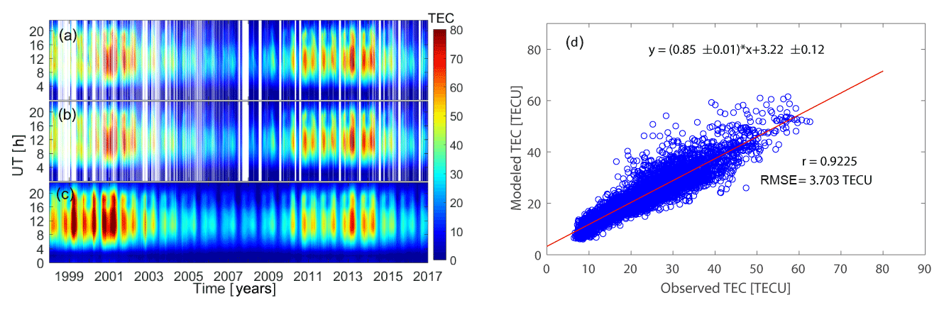
Figure 2 (a) GPS TEC, (b) reconstructed TEC and (c) modeled TEC over Malindi. (d) Correlation between EOF-modeled TEC and GPS-derived TEC over Malindi from 1999 to 2017.

3.3 Model validation

To asses the performance of the EOF-based TEC model, we compared the model results with the TEC derived from the IRI-2016 model and GIMs obtained from the website (ftp://ftp.aiub.unibe.ch/CODE/, last access: 20 April 2018) of the Center for Orbit Determination in Europe (CODE). From here onwards, the TEC from the EOF-based TEC model will be referred to as the EOF TEC, the TEC derived from the GPS receiver in Malindi as the GPS TEC, the TEC from CODE's GIMs as CODE's TEC and the TEC from the IRI-2016 model as the IRI TEC. We used both Kp and Dst to characterize the days into quiet and disturbed. A day was considered to be quiet if Kp ≤ 3 for all 3 h periods of the day.

3.3.1 Quiet days

Quiet days were selected from the equinox (March and September) and solstice (June and December) months of a high (2002) and low (2009) solar activity phases in order to validate the EOF-based TEC model. The data for the selected quiet days were excluded from the matrix used to generate the model coefficients, and the same procedure for model construction was repeated. The IRI TEC for the selected days was obtained from the web interface of the IRI-2016 model hosted at Omniweb (https://omniweb.gsfc.nasa.gov/vitmo/iri2016_vitmo.html, last access: 26 July 2018). To retrieve the IRI TEC, the location was specified to coincide with the geographic coordinates of the MAL2 GPS receiver, and the top-side boundary was set to its maximum value of 2000 km. The NeQuick option was used as the top-side electron density model, and ABT-2009 was used for the bottom-side thickness. Figure 3 shows hourly diurnal variation of the GPS TEC, IRI TEC, EOF TEC and CODE's TEC over Malindi for some selected quiet days. As expected, TEC values were higher in 2002 than in 2009. The IRI-2016 model overestimated the diurnal TEC over Malindi during the low solar activity year 2009 and during the winter solstice of the high solar activity year 2002. The overestimate of the GPS TEC by the IRI TEC is similar to what Olwendo et al. (2012) observed when they compared GPS TEC measurements over Kenya with the TEC from the IRI-2007 model. During the equinox months of higher solar activity years, IRI TEC values were higher and lower than the GPS TEC at about 03:00–09:00 and 11:00–13:00 UT respectively. The CODE's TEC overestimated the GPS TEC, especially during the high solar activity year 2002. The overestimate of the GPS TEC by CODE's TEC was not reflected much during the low solar activity year 2009. The EOF TEC, in contrast, replicated the diurnal TEC quite well, except on DOY 066 and DOY 339 in 2009. In general, the highest correlation was observed between the GPS TEC and CODE's TEC, followed by the correlation of the GPS TEC with the EOF TEC. It is worth noting that CODE's TEC mainly overestimated the TEC over Malindi, especially during higher solar activity years. Meanwhile, the IRI-2016 model overestimated the GPS TEC over MAL2 between 03:00 and 07:00 UT during high solar activity periods and throughout the day during lower solar activity years. This may be due to inadequate ingestion of ground-based data from the East African region in to the IRI model. As mentioned earlier, measurements from ionosondes were used to provide ground data during IRI model construction, and such data are currently limited over East Africa.

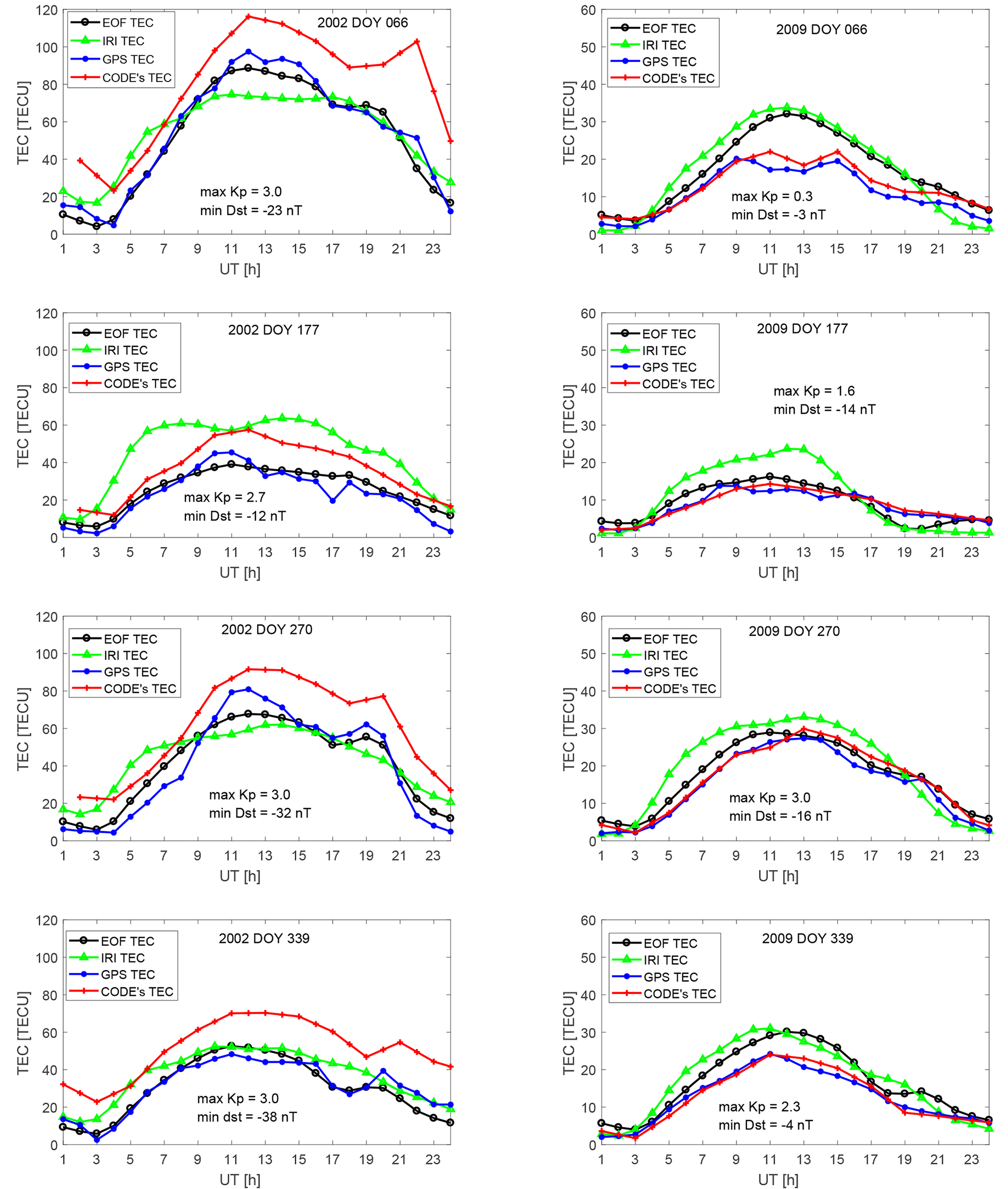
Figure 3 GPS TEC, IRI TEC, CODE's TEC and EOF TEC over Malindi for some selected quiet days. Included in each plot are the maximum Kp and the minimum Dst index for the day.

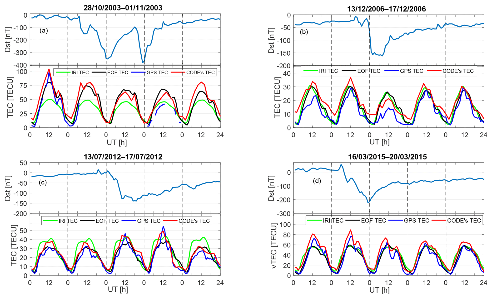
Figure 4 GPS TEC, IRI TEC, CODE's TEC and EOF TEC over Malindi for some selected storms. In these plots, the GPS TEC values are taken as a true representation of the ionosphere over Malindi. However, in the absence of GPS TEC (as in the case of the storm of 29–31 October 2003 shown in a), CODE's TEC was taken as the correct description of the ionospheric response to the storm.

3.3.2 Disturbed days

To study the storm time performance of the EOF-based TEC model, we simulated the TEC for some selected geomagnetic storms. As stated earlier, the test days were excluded in the process of generating the model coefficients. The IRI TEC for the storm days was obtained with the storm model turned on. The bottom panels of Fig. 4 show variation of the hourly diurnal TEC, while the top panels show variation of Dst index during some selected major geomagnetic storms. In Fig. 4a, TEC variation for a storm that occurred from 29–30 October 2003 is shown. No continuous GPS TEC measurements were available from MAL2 IGS receiver during this storm period. As can be seen in CODE's TEC, the storm had negative effect on the peak value of the TEC. The same negative storm effect was replicated by the EOF and IRI models, especially on 30–31 October 2003. Another major geomagnetic storm occurred in December 2006, with the main phase on 15 December 2006 (Fig. 4b). The EOF TEC, CODE's TEC and the IRI TEC on the day of the main phase of the storm showed negative storm effects, consistent with the GPS TEC. A case of a positive storm time effect on the ionosphere is shown in Fig. 4c, where the EOF TEC and CODE's TEC showed similar positive storm time effects to the GPS TEC. This was not reflected in the TEC derived from the IRI-2016 model. Shown in Fig. 4d is the TEC response to the geomagnetic storm that occurred in March 2015. During the recovery period, which lasted for many days, the GPS TEC showed negative storm effects compared to its value during the time of storm commencement. The EOF TEC, CODE's TEC and the IRI TEC all showed negative storm effects during the recovery period.

Figure 5 Diurnal variation of root-mean-square error (RMSE) of IRI TEC, CODE's TEC and EOF TEC relative to GPS TEC over Malindi.

3.3.3 Statistical analysis

From the EOF-based TEC model, we have simulated the TEC for the months of March, June, September and December for low (2009) and high (2013) solar activity years. In each of these simulations, the data for the selected months were excluded from the data used to generate the model coefficients. It is worthy noting that in generating the model coefficients, say for March 2009, only the data of March 2009 were excluded. The monthly median values for the EOF TEC, IRI TEC and CODE's TEC were used to compute the RMSE of the predicted TEC from the GPS TEC for every hour of the day. The diurnal variation of the RMSE values in 2009 and 2013 are shown in Fig. 5. From Fig. 5, the uncertainty in predicting the observed TEC was higher in 2013 than in 2009. This could be due to intensification of equatorial electrodynamic processes and the associated effects, such as TEC perturbations during higher solar activity years (Andima et al., 2015). These secondary effects of the equatorial dynamo processes are probably not well captured by the models. A comparison of the performance of the different models has shown that CODE's GIMs predicted the TEC over MAL2 with the least RMSE values, followed by the EOF model in 2009. The greatest uncertainty in predicting the TEC over MAL2 in the same year was observed in the IRI-2016 TEC. Similarly in 2013, the IRI TEC had higher RMSE values compared to the EOF TEC. CODE's GIMs showed the largest uncertainty in predicting the TEC over MAL2 during the December solstice of the high solar activity year 2013. The diurnal uncertainties in the ability of IRI-2016 to predict the TEC over MAL2 exhibited two peaks in March, June and September in 2009. The maximum RMSE values in the IRI-2016-predicted TEC were observed between 11:00 and 13:00 UT in March and June and between 13:00–14:00 UT in September in 2009. The December solstice showed a single peak in the RMSE values from 06:00–07:00 UT in 2009. Both the EOF TEC and CODE's TEC had the largest RMSE values from 11:00–14:00 UT in the same year. The RMSE values from 16:00–18:00 UT in March and September 2009 were much higher than those in June and December of the same year. In 2013, the RMSE in the IRI-2016-predicted TEC in the months of March and September had only single peaks which occurred at about 06:00 UT. However, two peaks, one between 04:00 and 07:00 UT and a second one between 13:00 and 14:00 UT, were observed in June and December 2013. The smallest error in the IRI TEC and the EOF TEC was observed after midnight local time to about 03:00 UT in both 2009 and 2013.

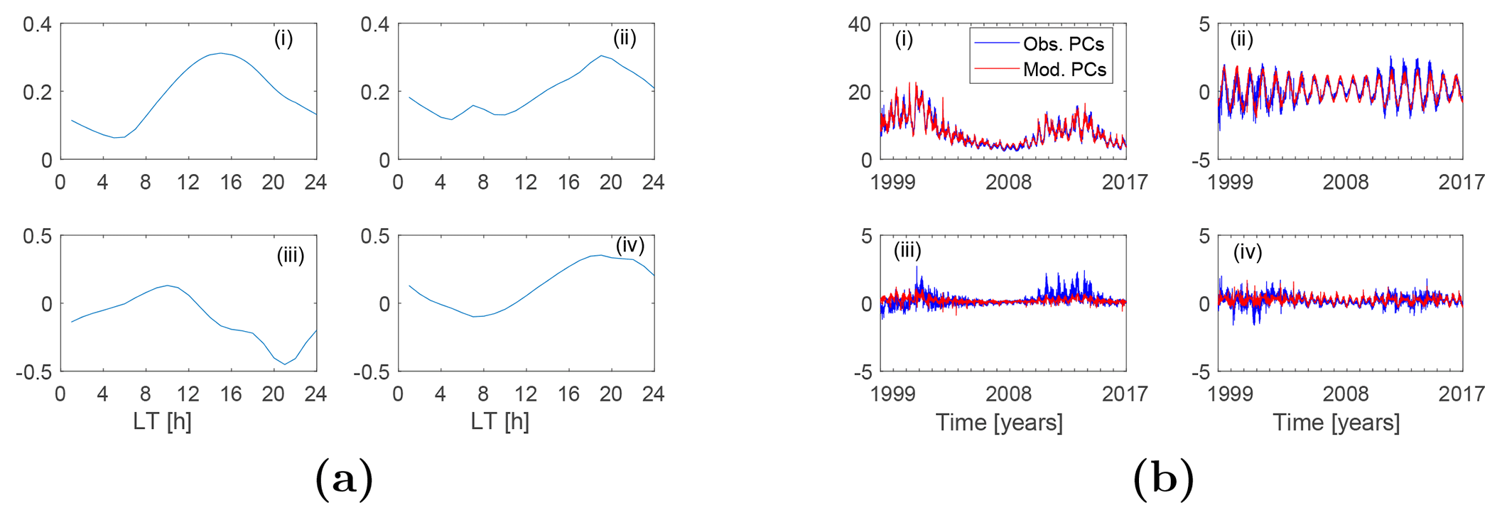
Figure 6 (a) The first basis modes of the first four first-layer expansion coefficients. (b) The expansion coefficients (blue) and their modeled values (red) for the basis modes in (a).

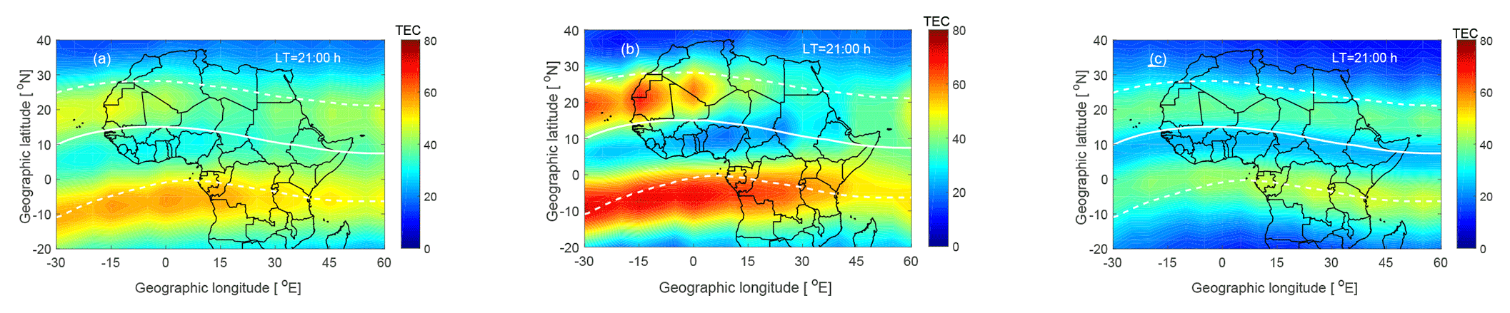
Figure 7 EOF TEC (a), CODE's TEC (b) and the IRI TEC (c) for the DOY 070 in 2015. Shown on the plots are the local times in hours. The horizontal curved solid white lines show the geomagnetic dip equator. The dashed white lines show the anomaly region at ±15^∘ geomagnetic latitude from the dip equator.

4 Modeling the TEC over African low latitudes

The first step in the regional TEC modeling was to extract the TEC for the African low-latitude region from CODE's GIMs. The daily GIMs were organized into bins of 2.5^∘ × 5^∘ × 1 h (latitude × longitude × LT). The binned data were then decomposed into the spatial and temporal components according to the equation

$$\begin{array}{}\text{(8)}& {\displaystyle }\mathrm{TEC}(\mathrm{lat},\mathrm{lon},\mathrm{LT},m)=\sum _{i=\mathrm{1}}^r{U}_i(\mathrm{lon},\mathrm{lat})\times P_i(\mathrm{LT},m).\end{array}$$

In Eq. (8), U_i(lon,lat) is the basis modes representing the spatial TEC variability, and P_i(LT,m) is the coefficients that describe the temporal TEC variations in terms of local time (LT) and month (m). The temporal component in Eq. (8) was further broken into the diurnal and long-term (seasonal, annual and solar cycle) variations by another decomposition which we refer to here as the second-layer decomposition expressed as

$$\begin{array}{}\text{(9)}& {\displaystyle }{P}_i(\mathrm{LT},d)=\sum _{i,j=\mathrm{1}}^m{U}_{i,j}\left(\mathrm{LT}\right)\times A_{i,j}\left(d\right).\end{array}$$

In Eq. (9), U_i,j(LT) is the basis functions of the ith first-layer coefficients, and A_i,j(d) is the coefficients of U_i,j(LT). Figure 6a shows the first basis modes for each of the first four expansion coefficients in the first-layer decomposition. Equations (5)–(7) were then used to model the coefficients A_i,j(d). Figure 6b shows the coefficients A_i,j(d) together with their model-predicted values. Using the modeled values of the coefficients, the regional TEC was then reconstructed in a reverse order. We first used Eq. (9) to obtain the coefficients for the first-layer decomposition and then applied Eq. (8) to determine the TEC in each grid cell. Figure 7 shows the modeled TEC, CODE's TEC and the IRI TEC for DOY 070 in 2015. It can be seen from Fig. 7 that the model has reproduced the main features of the EIA region quite well. Higher correlations are observed between the EOF-modeled TEC and CODE's TEC (Fig. 7a and b). This high correlation is an indication that the model-predicted results could offer a good alternative to estimating the background TEC, since CODE's TEC is derived from GNSS measurements.

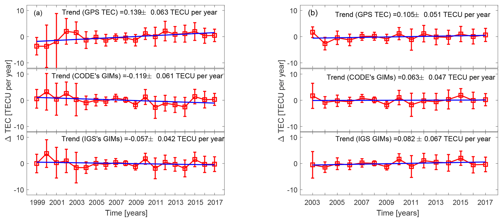
Figure 8 The yearly median residual TEC after removing the solar and magnetic activity variations for the periods 1999–2017 (a) and 2003–2017 (b). The upper panels are for the TEC derived from MAL2 IGS receiver, the middle panels are for TEC from CODE's GIMs and the lower panels are for TEC from IGS GIMs corresponding to the location of MAL2 IGS receiver. The straight lines in these plots are the first-degree polynomial fits used to estimate the trends.

Figure 9 Trends in TEC over the African low-latitude region derived from CODE's (a, b) and IGS (c, d) GIMs. Panels (a) and (c) are for the period 1999–2017 while (b) and (d) are for the period 2003–2017. The horizontal curved white lines are same as described in Fig. 7.

5 TEC trends

In the past, few studies (e.g., Lean et al., 2011; Lastovicka et al., 2017) have derived long-term TEC trends, and these mainly used TEC data from GIMs. In this work, we have used the GPS-derived TEC and GIMs to study TEC trends over the low-latitude region of Africa. A key aspect in trend studies is the art of suppressing the solar and magnetic activity influences on these trends. We used the EOF-modeled TEC as background the TEC to remove the solar and magnetic effects in influencing the TEC trends. First, the monthly median TEC values were calculated from the daily TEC. The median TEC values were then modeled using similar equations as in Eqs. (5)–(7). In these equations, the daily inputs were replaced with their monthly averages. The modeled TEC values were then subtracted from the monthly medians to obtain the TEC residuals. The monthly TEC residuals from 10:00–14:00 LT were averaged for each year to give a representation of the noontime annual TEC residuals (ΔTEC). The trend was then determined using the equation (Lastovicka et al., 2006; Bremer et al., 2012)

$$\begin{array}{}\text{(10)}& {\displaystyle }\mathrm{\Delta }\mathrm{TEC}=A+B\cdot \mathrm{time}\left(\mathrm{year}\right),\end{array}$$

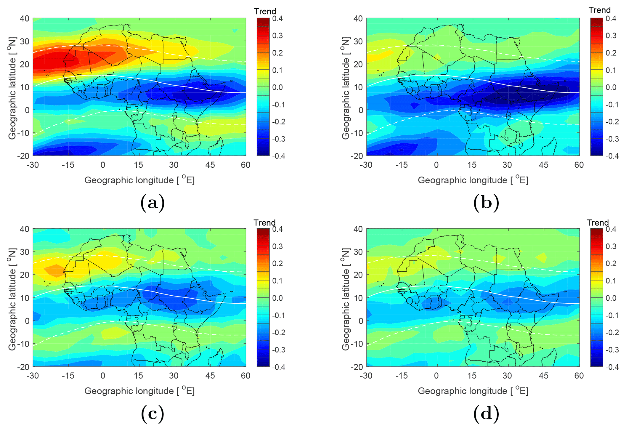
where A is the constant part, and B is the slope (trend) of the time-dependent TEC residuals. Lastovicka et al. (2017) attributed the positive global TEC trends reported in Lean et al. (2011) to lower TEC values in CODE's GIMs, especially prior to 2003. To test this assertion, we have estimated the long-term trends in the TEC for the periods 1999–2017 and 2003–2017 using the GPS-derived TEC, CODE's TEC and the TEC from IGS GIMs. Figure 8 shows the TEC trends obtained from the GPS-derived TEC and the TEC from GIMs of CODE and IGS over Malindi. Trends of 0.139±0.063, $-\mathrm{0.119}\pm \mathrm{0.061}$ and $-\mathrm{0.057}\pm \mathrm{0.042}$ TECU yr⁻¹ were obtained using the GPS TEC, CODE's GIMs and IGS GIMs over Malindi respectively. Though the trend values in Fig. 8a were slightly different, their 95 % confidence bounds reveal a slight positive TEC trend for the period 1999–2017. For the period 2003–2017, the trend estimates from the three data sets show that TEC trends over MAL2 are positive. To study the trends in the TEC over the African low-latitude region, we used the GIMs and estimated the trends in each of the 2.5^∘ × 5^∘ (latitude × longitude) grids. The trends are shown in Fig. 9a and c for the period 1999-2017 and in Fig. 9b and d for the period 2003–2017. The trends in Fig. 9 show a latitudinal dependence, with the trends in the vicinity of the crest of the EIA region being more positive than those near the magnetic equator, where the trend was negative over most of the African equatorial region. Analysis of the data from 1999–2017 revealed higher average values of TEC trends than that from 2003–2017 for both CODE's and IGS GIMs, though the general pattern of the trends remained unchanged. The trend pattern observed in this study confirms the latitudinal variation in TEC trends reported in Lean et al. (2011). The difference in the trend magnitudes for the periods 1999–2017 and 2003–2017 could be as pointed out earlier due to a bias towards lower values of GIMs prior to 2002 (Lastovicka et al., 2017; Emmert et al., 2017). If so, the trends in the TEC over African low latitudes are therefore mainly negative, though cases of slight positive trends are also possible, especially at the crest of the EIA region. Geomagnetic or anthropogenic factors are often the plausible physical mechanisms for explaining trends in upper atmospheric parameters. The anthropogenic contributions to trends arise through the accumulation of greenhouse gases, which result in a decrease of atomic oxygen in the upper atmosphere. While the geomagnetic control of the trends is either due to the long-term changes in geomagnetic activity (Danilov and Mikhailov, 1999; Mikhailov and Marin, 2000) or to Earth's magnetic field secular variations (Foppiano et al., 1999; Gnabahou et al., 2013), the latter view may explain the latitudinal dependence in the trends over the African low-latitude region. However, a detailed study is required to quantify the relative contribution of the different trend drivers over the African low latitudes.

6 Summary and conclusion

We have used EOF expansion together with least-squares regression to model the TEC over the African low-latitude region. We first developed a single-station model over MAL2, a station at the southern crest of the EIA, and then constructed a regional model to predict the TEC over the African low latitudes. Despite the complicated nature of the low-latitude ionosphere, the model over MAL2 was able to satisfactorily reproduce the diurnal, seasonal and solar activity variations in the observed TEC. Comparison of the model results with IRI-2016-derived TEC showed that the EOF-based TEC model was more accurate in predicting the daytime TEC over Malindi than IRI-2016. In contrast, CODE's GIMs were better correlated with GPS TEC than the TEC from the EOF-based model, though CODE's GIMs mainly overestimated the GPS TEC over MAL2 during higher solar activity years. The large discrepancy of the IRI-2016-predicted daytime TEC from the observed TEC over MAL2 during periods of low solar activity and during the winter solstice could be due to the overrepresentation of the effects of the low-latitude E×B plasma drifts and thermospheric winds in the model. The regional model reproduced the known features of the low-latitude ionosphere quite well. Using the TEC from the EOF-based model as the background TEC to suppress solar and magnetic activity dependence of the TEC, we estimated trends in the TEC over the African low-latitude region. The regional trends showed a latitudinal dependence, with the trends in the vicinity of the magnetic equator being more negative than those at the crest of the EIA.