Comparisons between the WRF data assimilation and the GNSS tomography technique in retrieving 3-D wet refractivity fields in Hong Kong

Water vapor plays an important role in various scales of weather processes. However, there are limited means to accurately describe its three-dimensional (3-D) dynamical changes. The data assimilation technique and the Global Navigation Satellite System (GNSS) tomography technique are two of the limited means. Here, we conduct an interesting comparison between the GNSS tomography technique and the Weather Research and Forecasting Data Assimilation (WRFDA) model (a representative of the data assimilation models) in retrieving wet refractivity (WR) in the Hong Kong area during a wet period and a dry period. The GNSS tomography technique is used to retrieve WR from the GNSS slant wet delays. The WRFDA is used to assimilate the zenith tropospheric delay to improve the background data. The radiosonde data are used to validate the WR derived from the GNSS tomography, the WRFDA output, and the background data. The root mean square (rms) of the WR derived from the tomography results, the WRFDA output, and the background data are 6.50, 4.31, and 4.15 mm km⁻¹ in the wet period. The rms becomes 7.02, 7.26, and 6.35 mm km⁻¹ in the dry period. The lower accuracy in the dry period is mainly due to the sharp variation of WR in the vertical direction. The results also show that assimilating GNSS ZTD into the WRFDA only slightly improves the accuracy of the WR and that the WRFDA WR is better than the tomographic WR in most cases. However, in a special experimental period when the water vapor is highly concentrated in the lower troposphere, the tomographic WR outperforms the WRFDA WR in the lower troposphere. When we assimilate the tomographic WR in the lower troposphere into the WRFDA, the retrieved WR is improved.

1 Introduction

Water vapor (WV), mostly contained in the troposphere, plays an important role in various scales of atmospheric processes. But due to its active nature, there are limited models and techniques that can accurately describe or monitor its three-dimensional (3-D) dynamical changes (Rocken et al., 1993).

The development of the Global Navigation Satellite System (GNSS) technique and the densely deployed GNSS receivers provide us with the opportunity to monitor the WV fields in near real time. When the GNSS signal travels through the neutral atmosphere, it undergoes time delay and bending due to atmospheric refractivity. This effect is usually called the tropospheric delay in the GNSS community (Altshuler, 2002). The tropospheric delay is usually considered the product of the zenith delay and the mapping function (Lanyi, 1984; Niell, 1996). The zenith tropospheric delay (ZTD) consists of two parts: the hydrostatic part and the wet part. The wet delay is mainly associated with the WV and reflects WV content in the troposphere. Bevis et al. (1992) introduced the principle of using GNSS zenith wet delay (ZWD) to retrieve the precipitable water vapor (PWV). Since then, many scientists have carried out the GNSS PWV experiments (Askne and Nordius, 1987; Bokoye et al., 2003; Yao et al., 2014; Lu et al., 2015; Shoji et al., 2016). Now, the GNSS PWV can be retrieved with an uncertainty of 1–2 mm in post-processing (Tregoning et al., 1998; Adams et al., 2011; Grejner-Brzezinska, 2013) or real-time modes (Yuan et al., 2014; Li et al., 2014, 2015).

The GNSS WV tomography technique was first proposed to monitor the 3-D or 4-D WV in 2000 (Flores et al., 2000; Seko et al., 2000; Hirahara, 2000). Since then, many scientists have proposed refined methods to improve the GNSS WV tomography (Flores et al., 2001; Nilsson and Gradinarsky, 2006; Rohm and Bosy, 2011; Wang et al., 2014a, b; Zhao and Yao, 2017). The tomographic inversion algorithm can be roughly categorized into two groups. One group solves the tomography equation in the least squares scheme or in the Kalman filter scheme with additional constraints or using a priori information (Flores et al., 2000; Rohm and Bosy, 2011; Cao et al., 2006; Zhang et al., 2017). The other group uses the algebraic reconstruction algorithm or similar methods (Bender et al., 2011; Wang et al., 2014b; Zhao and Yao, 2017). Some scientists also use different methods from above to solve the GNSS WR tomography problem (Nilsson and Gradinarsky, 2006; Perler et al., 2011a; Altuntac, 2015). Besides the algorithm improvement, some scientists tried to optimize the voxel division (Chen and Liu, 2014), use virtual reference stations (Adavi and Mashhadi-Hossainali, 2014) or use additional GNSS rays (Zhao and Yao, 2017) to increase the effective GNSS rays and thus improve the tomography results. Though the tomography technique has the advantages of (1) being free of weather conditions and (2) retrieving 3-D WR fields in near real time, it still suffers from some problems. The sparse distribution of the GNSS receivers and the bad satellite-receiver geometry lead to serious ill-posed and ill-conditioned problems, and also limit the WR retrieval resolution in both vertical and horizontal domains.

Besides the GNSS tomography technique, the WR can also be retrieved by data assimilation which is based on numerical weather prediction (NWP) models (Perler et al., 2011b). The Weather Research and Forecasting (WRF) model is a state-of-the-art atmospheric modeling system that is used to simulate the dynamic processes of the atmosphere (Jankov et al., 2005; Carvalhoaabc, 2012). It is mainly developed and supported by the Mesoscale and Microscale Meteorology (MMM) Laboratory of the National Center for Atmospheric Research (NCAR). And the WRF data assimilation (WRFDA) is designed to obtain the best estimate of the actual atmospheric state at any analysis time (Barker et al., 2004, 2012; Huang et al., 2008; Singh et al., 2017). Many studies have demonstrated that assimilating ZTD/PWV into WRFDA can improve the reanalysis water vapor field (Pacione et al., 2001; Faccani et al., 2005; Bennitt and Jupp, 2012; Moeller et al., 2016; Lindskog et al., 2017). Besides the WRFDA model, the Japan Meteorological Agency (JMA) Mesoscale Numerical Weather Prediction Model (Nakamura et al., 2004) and AROME NWP system (Boniface et al., 2009) can also make use of ZTD/PWV data assimilation.

Though the GNSS tomography technique and the data assimilation technique belong to different fields, both of them could retrieve 3-D WR fields. It will be interesting to compare their capabilities in retrieving WR fields under different weather conditions and to explore the feasibility of combining them. Such results may provide insights for the NWP community into this new technique and the possibility of assimilating the tomography results into the NWP models. For the GNSS community, they will get a better understanding of the WRF data assimilation and its capability in simulating the water vapor field. For this purpose, we conduct GNSS tomography and data assimilation experiments in the Hong Kong area using the SatRef network in a wet period and a dry period. WR fields retrieved from GNSS tomography and WRFDA outputs are validated by the radiosonde data. We also explore the feasibility of assimilating the GNSS tomographic WR into the WRFDA to further improve the WR field.

2 Research area and data analysis

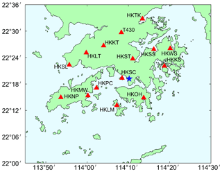
The study area is within 113.75–114.5^∘ E and 22–22.6^∘ N as shown in Fig. 1. There are 15 continuous GNSS stations belonging to the Hong Kong SatRef network deployed in the study area. They are all equipped with Leica GNSS receivers and antennas to receive the GNSS signals and automatic meteorological devices to record the temperature, pressure, and relative humidity. The average inter-distance between stations is about 10 km. The altitudes of the highest station (HKNP) and the lowest station (HKLM) are 354 and 10 m. In GNSS tomography, we regard a network whose altitude differences of its stations are less than 1 km as a flat network. Therefore, the SatRef network is a flat network.

Two periods of GNSS observation data are processed to generate ZTD and slant wet delay (SWD). One is a wet period from 20 to 26 July 2015 when Hong Kong suffered the heaviest daily rainfall of 2015 (191.3 mm rainfall on 22 July). The other is a dry period from 1 to 7 August 2015 when Hong Kong is rainless. The details about the GNSS data processing and the SWD reconstruction can be found in Appendix A.

Figure 1 Research area of the experiment. The red triangles indicate the GNSS stations and the blue star indicates the radiosonde station in Hong Kong.

Figure 2 Flowchart of data assimilation using the WRF model.

3 Method

3.1 WRF data assimilation

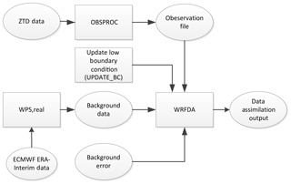
WRF model version 3.7 is used in this study. WRFDA-3DVAR is used to assimilate the GNSS ZTD to improve the background data. The horizontal resolution of WRFDA output is set to 3 km. And the atmosphere is vertically divided into 45 layers. The pressure of the top layer is 50 hpa. There are 10 layers in the planetary boundary layer (PBL). We use the ZTD error output by the Bernese 5.0 software as the observation error. We use the reanalysis data from European Center for Medium-Range Weather Forecasts (ECMWF) ERA-Interim pressure levels and surface data as the background data, whose spatial resolution is $\mathrm{0.75}{}^{\circ }\times \mathrm{0.75}{}^{\circ }$. And we run the WRFDA model at 00:00 and 12:00 UTC, corresponding to the radiosonde observation time. The procedures to do the assimilation experiments are shown in Fig. 2.

The background data are processed by the WRF Preprocessing System (WPS). The WRFDA is run with the generic CV3 option, and the default background error is adopted in this study. The GNSS ZTDs are the input observations for WRFDA. We run WRFDA to obtain the data assimilation output, labeled Output1. The output from the WPS and real.exe is labeled Output2. We compare the WR derived from Output1 and Output2. We use Eq. (1) to calculate WR (Vedel and Huang, 2004) from Output1 and Output2.

$$\begin{array}{}\text{(1)}& {\displaystyle }\mathrm{WR}={\displaystyle \frac{P_{\mathrm{w}}}{T}}\times \left(k_{\mathrm{1}}+{\displaystyle \frac{k_{\mathrm{2}}}{T}}\right),\end{array}$$

where P_w is the water vapor pressure in each grid point in Pascal, and T is the temperature in each grid point in Kelvin. $k_{\mathrm{1}}=\mathrm{2.21}\times {\mathrm{10}}^{-\mathrm{7}}$ K Pa⁻¹; $k_{\mathrm{2}}=\mathrm{3.73}\times {\mathrm{10}}^{-\mathrm{3}}$ K² Pa⁻¹. We use Eq. (2) to calculate P_w.

$$\begin{array}{}\text{(2)}& {\displaystyle }{P}_{\mathrm{w}}={\displaystyle \frac{p\times q}{\mathrm{0.622}}},\end{array}$$

where p is the pressure in Pascal and q is the specific humidity in g g⁻¹.

The WRFDA has many options for different physical parameterizations. In order to find the best choice for the data assimilation experiment, we follow Chien et al. (2006) to set 12 schemes to do the sensitivity tests, which are listed in Table 1. We carry out the sensitivity test at 00:00 UTC 22 July 2015. The domain size is set to 30×24 grids which just cover the study area. The grid size is 3 km × 3 km. We run WRFDA using the different setting schemes. The radiosonde data are used to validate the wet refractivity derived by the WRFDA output. Table 1 shows that all schemes have the same bias, standard deviation (SD), and root mean square (rms), which suggests that the output wet refractivity is not affected by the physical parameterization settings in WRFDA.

In this study, we use the Kain–Fritsch scheme (Kain and Frisch, 1990), WRF Single-Moment (WSM) 5-class scheme (Hong et al., 2004) and Yonsei University PBL scheme (Hong et al., 2006), which are the same as Chien et al. (2006). The other physical options include the unified Noah land-surface model (Tewari et al., 2004) and the revised MM5 Monin–Obukhov scheme (Monin and Obukhov, 1954). The Rapid Radiative Transfer Model (Mlawer et al., 1997) and Dudhia's scheme (Dudhia, 1989) are used for longwave radiation and shortwave radiation, respectively.

Table 1 Physical parameterization schemes and statistics of bias, rms, and SD of retrieved WR using different schemes. Unit is mm km⁻¹.

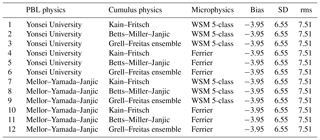
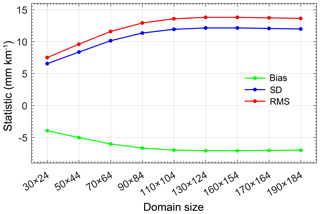
In order to figure out how sensitive the wet refractivity output is to the domain size, we carry out another sensitivity test at 00:00 UTC 22 July 2015. And we increase the domain size gradually from 30×24 grids to 190×184 grids. In each run, we validate the wet refractivity derived by the WRFDA output using the radiosonde data. The statistical results of the sensitivity tests are shown in Fig. 3. It shows that the smaller domain size has the smaller bias, SD, and rms. So, the domain size of the data assimilation experiment is set to 30×24 grids which just cover the study area.

3.2 GNSS tomography

The limited number of stations, flat vertical distribution of stations, and bad satellite-station geometry impose serious ill-posed problems in the WR tomography. To handle this problem well, we use the tomography method proposed by Zhang et al. (2017). This method is based on the adaptive Laplacian smoothing and Helmert variance component estimation. It also uses the meteorological data from each GNSS station to constrain the WR near the ground. This tomography strategy is free of a priori information, which makes it an independent technique and thus ensures the fairness when the tomography technique is compared with the WRFDA model. The WR can be retrieved directly by this tomography strategy when the SWDs are used as observations. The troposphere is vertically divided into 13 layers with a constant thickness of 800 m, and horizontally divided into grids whose resolution is ∼10 km in the longitudinal direction and ∼8 km in the latitudinal direction. The tomography algorithm is described as follows:

$$\begin{array}{}\text{(3)}& \left.\begin{array}{c}\mathit{Y}=\mathbf{A}\mathit{X}\\ \mathbf{0}=\mathbf{V}\mathit{X}\\ \mathbf{0}=\mathbf{H}\mathit{X}\\ \mathbf{0}=\mathbf{B}\mathit{X}\\ {\mathit{X}}_m=\mathit{X}\end{array}\right\},\end{array}$$

where the first equation is the observation equation, Y is the vector of SWDs, A is the design matrix consisting of intercepts in each voxel, and X is the vector of WR in each voxel. The second to fourth equations in Eq. (1) are the vertical, horizontal, and boundary constraints. The fifth equation is used to constrain the WR near the ground using the meteorological data at each GNSS station. V, H, and B are the design matrices for constraint equations. The boundary constraints are established by setting the WR in the top layer to 0. The vertical and horizontal constraints are established by Laplacian smoothing in the vertical and horizontal directions, respectively. The Laplacian smoothing can be described as

$$\begin{array}{}\text{(4)}& x_{\mathrm{1}}+x_{\mathrm{2}}+x_{\mathrm{3}}+x{}_{\mathrm{4}}-q{x}_{\mathrm{0}}=\mathrm{0},\end{array}$$

where the WR x₀ equals the weighted average WR of its nearest four voxels in the same plane, and q is the smoothing factor.

In a least square scheme, the solution can be found by

$$\begin{array}{ll}{\displaystyle }\mathit{X}& {\displaystyle }=({\mathbf{A}}^T\mathbf{A}+{\mathit{\lambda }}_{\mathrm{1}}{\mathbf{V}}^T\mathbf{V}+{\mathit{\lambda }}_{\mathrm{2}}{\mathbf{H}}^T\mathbf{H}+{\mathit{\lambda }}_{\mathrm{3}}{\mathbf{B}}^T\mathbf{B}+{\mathit{\lambda }}_{\mathrm{4}}{)}^{-\mathrm{1}}\\ \text{(5)}& {\displaystyle }& {\displaystyle }\cdot ({\mathbf{A}}^T\mathit{Y}+{\mathit{\lambda }}_{\mathrm{4}}{\mathit{X}}_m),\end{array}$$

where λ_i (i=1, 2, 3, 4) are the weights of corresponding constraints.

In Zhang et al. (2017), the solution is found in an iterative feedback–update process, which is simply described as follows.

• a.

  Establish the initial constraints and initialize their weights as 1, namely ${\mathit{\lambda }}_{\mathrm{1}}={\mathit{\lambda }}_{\mathrm{2}}=\mathrm{1}$; λ₃ is set to a large value; λ₄ is set to 1; λ₃ and λ₄ are not updated in the following run.

• b.

  Determine the values of λ₁ and λ₂ by the Helmert variance component estimation method and calculate the tomography solutions by Eq. (3).

• c.

  Update the smoothing factors by using the solutions in b:

  $$\begin{array}{}\text{(6)}& q=\left\{\begin{array}{ccc}n& \mathrm{if}& x_{\mathrm{0}}<x_m\\ {\displaystyle \frac{\sum _{i=\mathrm{1}}^n{x}_i}{x_{\mathrm{0}}}}& \mathrm{if}& x_{\mathrm{0}}>x_m\end{array}\right.,\end{array}$$

  where n is the number of voxels used to calculate the weighted average. x_m is a threshold set to prevent updating the smoothing factor by inaccurate solutions. The initial value for x_m is half of the maximum wet refractivity in the solutions. x_m is updated by multiplying x_m by a scale factor, say 0.9, after each run until it is no larger than 3 times the mean square error of X.

• d.

  Use the new smoothing factors in c to update the horizontal and vertical constraints and redo b and c until the mean square error of the solution differences between this run and the previous run approaches a stable value. In practice, we set a threshold of 20 iterations, which is enough to ensure a stable solution.

Figure 3 WR statistics of the sensitivity test of domain size validated by radiosonde data.

4 Results

The radiosonde data are used to validate the WR derived from GNSS tomography, Output1 and Output2. Since the radiosonde launches at 00:00 and 12:00 UTC daily, the WR at these epochs is validated. Equation (1) is also used to calculate WR from radiosonde data. The vertical coordinates of Output1 and Output2 are converted to geopotential heights by the NCAR Command Language (NCL) (UCAR/NCAR/CISL/VETS, 2013) and the geodetic heights of tomographic results are converted to normal height. The slight differences between geopotential heights and normal heights are neglected. We interpolate the radiosonde to tomographic nodes since the former has a much higher resolution ∼23 layers from 0 to 10 km height than the latter (13 layers) and thus we can get a higher interpolation accuracy. We use a bilinear interpolation method in the horizontal domain and a linear interpolation method in the vertical direction. By these methods, we interpolate the WR derived from the Output1, Output2 and radiosonde data to the tomography nodes. Finally, the WR is validated by the radiosonde data. For simplicity, WR from radiosonde data and GNSS tomography are denoted as “radiosonde” and “tomography” hereinafter.

Figures 4 and 5 show the vertical profiles of the radiosonde, Output1, Output2 and the tomography in the July and August periods, respectively. Output1, Output2, and the tomography agree well with the radiosonde, which indicates that these three methods successfully retrieved the vertical profile of the WR. It is also observed that Output1, Output2, and the tomography agree better with the radiosonde in the July period than in the August period. This difference should be due to the vertical distribution of WR. Though Hong Kong suffered heavy rain in the July period, the WR was more evenly distributed from 0 to 10 km height than that in the August period. In the dry August period, the WR was highly concentrated in the lower troposphere (<6 km) and its vertical changes were very sharp. This situation decreased the performance of the tomography technique and the data assimilation technique. This also indicates that the tomography technique has decreased capabilities in retrieving WR in a highly changing troposphere. Compared with Output2, Output1 is slightly improved by reducing the mean absolute error (MAE) by 1.25 mm km⁻¹. The difference between the tomography and Output1 is obvious at some time epochs in the dry period (e.g., 12:00 on 4 and 5 August).

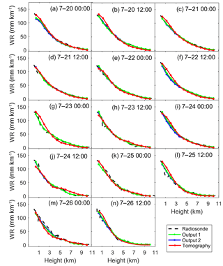
Figure 4 Comparisons among WR derived from Output1, Output2, tomography, and radiosonde in the wet period, 2015.

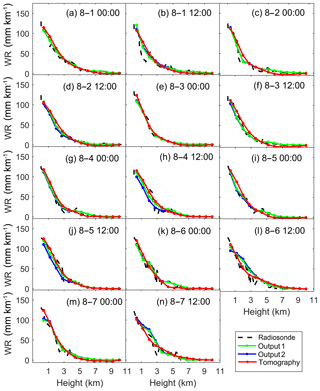
Figure 5 Comparisons among WR derived from Output1, Output2, tomography, and radiosonde in the dry period, 2015.

Figure 6 shows the statistics of the bias, SD, and rms of the tomography, Output1, and Output2 validated by the radiosonde at different heights. In the wet period, bias of Output1 is smaller than that of Output2, but the differences are not obvious in terms of SD and rms. In the dry period, the bias of Output1 in the lower troposphere is slightly greater than that of Output2. Overall, the differences between Output1 and Output2 are not significant.

In the wet period, the bias, SD, and rms of the tomography are greater than that of Output1 most of the time. But in the dry period, the SD and rms of the tomography tend to be smaller than that of Output1 in the lower troposphere, but its bias is still greater. In general, the WRFDA performs better than the tomography technique in most of the cases, but the rms of tomography validated by the radiosonde at 400, 1600 and 2400 m height is smaller than WRFDA output as shown in Fig. 6f. So, in the lower troposphere in the dry period the tomography performed better than the WRFDA in terms of rms.

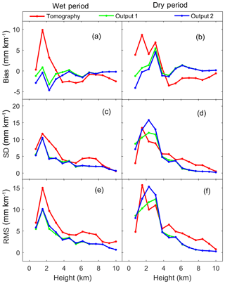
Figure 6 Statistics of bias, SD, and rms of the tomography, Output1, and Output2 validated by the radiosonde.

Table 2 shows the bias, SD, and rms of the tomography, Output1, and Output2 validated by the radiosonde. In the whole troposphere in the wet period, the tomography has the smallest bias but the largest SD and rms. Output1 and Output2 have the similar SD and rms that are much smaller than that of the tomography. But Output2 has the largest bias than Output1 and the tomography. In the lower troposphere in the wet period, Output1 has the smallest SD and rms, while the tomography has the largest ones. The bias of tomography is positive in the lower troposphere but negative in the upper troposphere; this should be due to the vertical smoothing constraints imposed on the WR. In the upper troposphere in the wet period, the tomography has the largest bias, SD, and rms, while Output1 has the smallest ones. Overall, both the tomography and the WRFDA results have larger bias, SD, and rms in the lower troposphere than in the upper troposphere, indicating that both the tomography technique and the data assimilation technique have deceased capabilities in the lower troposphere.

In the whole troposphere in the dry period, Output2 has the smallest bias but the largest SD and rms. The SD and rms of the tomography are larger than Output1. In the lower troposphere in the dry period, Output2 has the largest rms and SD, while Output1 has the smallest ones. In the lower troposphere in the dry period, the performance of the tomography is not as good as Output1 in terms of rms. However, in the upper troposphere in the dry period, the tomography has relatively larger bias, SD and rms than the WRFDA results.

Table 2 Statistics of bias, rms and SD of tomography, Output1 and Output2 validated by the radiosonde WR. Unit is mm km⁻¹.

Figure 7 Differences between WR obtained by various methods and radiosonde WR.

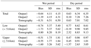
In general, assimilating GNSS ZTD into the WRFDA has slightly improved the WR retrieval by decreasing the rms by 0.2 mm km⁻¹. The WR derived from Output1 and Output2 has apparently smaller rms than the tomographic WR (4.15 mm km⁻¹ vs. 6.50 mm km⁻¹ and 4.31 mm km⁻¹ vs. 6.50 mm km⁻¹, respectively). The results obtained from WRFDA and tomography are better in the wet period than in the dry period, which is mainly due to the sharp vertical variation of WR in the dry period.

5 Discussion

In the dry period, due to the sharp vertical variations of WR, the tomography and Output1 have decreased performance in retrieving the WR, especially in the lower troposphere. Compared with the results in the wet period, the rms of the tomography and Output1 increases by 0.94 and 3.24 mm km⁻¹ in the dry period, respectively. The accuracy decrease is more significant in Output1 than in the tomography, resulting in the tomographic WR becoming better than Output1 (Fig. 6d and f) in the lower troposphere.

When assimilating ZTD into the WRFDA, we only use the total water vapor and cannot use the vertical profile of water vapor. This leads to the assimilation of ZTD having limited improvement in retrieving the vertical structure of the WR. Therefore, it is natural to consider assimilating the tomographic WR into the WRFDA to improve the retrieval of the vertical structure of WR. At present, WRFDA could not assimilate WR directly, but can assimilate meteorological parameters such as relative humidity, temperature and pressure. To assimilate the tomographic WR, we convert WR to relative humidity.

The relationship between relative humidity (RH) and P_w is shown as Eq. (7).

$$\begin{array}{}\text{(7)}& {\displaystyle }\mathrm{RH}={\displaystyle \frac{P_{\mathrm{w}}}{P_{\mathrm{s}}}},\end{array}$$

where P_s is the saturated water vapor pressure which is related to temperature and can be calculated by the Wexler formula (Wexler, 1976, 1977). The P_w is calculated by Eq. (1). The needed temperature and pressure data are from Output2.

After converting the tomographic WR to RH, we assimilate the RH together with the corresponding temperature and pressure into the WRFDA. Then, the similar procedures as described in Sect. 3.1 are performed to generate new WRFDA output.

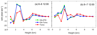
The tomography agrees better with the radiosonde than Output1 and Output2 in the lower troposphere below 3 km at 12:00 on 6 August (Fig. 5l) and at 12:00 on 7 August (Fig. 5n). So, we assimilate the tomographic WR below 3 km into the WRFDA at these two epochs. The generated output data are denoted as “Output3”. The difference between Output3 and radiosonde is denoted as “DA-Tomo”. The difference between Output1 and radiosonde is denoted as “DA-ZTD”. The difference between tomography and radiosonde is denoted as “Tomo”. The MAE at different heights at 12:00 on 6 and 7 August is shown in Fig. 7.

Figure 7 shows that the DA-ZTD is very close to the DA-Tomo. The MAE of the DA-ZTD is 6.04 mm km⁻¹ and the MAE of the DA-Tomo is 5.92 mm km⁻¹. This indicates that assimilating tomographic WR into the WRFDA can slightly improve the WR retrieval. But the large uncertainty (8.35 mm km⁻¹) of tomography WR in the lower troposphere limits the improvement.

6 Conclusions

GNSS WR tomography and data assimilation experiments are conducted in Hong Kong during a wet period and a dry period to test the capabilities of the tomography technique and the WRFDA in retrieving WR. The results show that both the tomography technique and the data assimilation technique can retrieve WR that agrees well with the radiosonde data.

In the wet period in the whole troposphere, the rms of tomography, Output1 and Output2 is 6.50, 4.31, and 4.15 mm km⁻¹. The rms becomes 7.02, 6.35, and 7.26 mm km⁻¹ in the dry period. Both methods obtained better WR in the wet period than in the dry period. We infer that the sharp vertical variations of WR reduced the WR retrieving accuracy in the dry period. In most of the cases, Output1 outperforms the tomographic WR, but the tomographic WR is better than Output1 in the lower troposphere in the dry period. By assimilating better tomographic WR in the lower troposphere into the WRFDA, we slightly improve the retrieved WR.

The above results suggest that both the WRFDA and the tomography technique can retrieve good WR but also have drawbacks. If we combine the two by assimilating good tomographic WR into the WRFDA, we may further improve the performance of the WRFDA in retrieving the water vapor field.

Appendix A

The GNSS observation data are processed by the precise point positioning module in Bernese 5.0 software using the same settings as detailed in Zhang et al. (2017). The International GNSS Service final orbit and clock products are used. The differential code biases (DCBs) are corrected by products from the Center for Orbit Determination in Europe. Antenna phase center offsets and variations, phase wind-up, Earth tides, Earth rotation, ocean tides and relativistic effects are corrected by conventional methods detailed in Kouba and Héroux (2001). We use the ionosphere-free combination of double frequencies to eliminate the first-order ionospheric delay and the higher-order terms are ignored. The tropospheric delay models are the Saastamoinen model (Saastamoinen, 1972) and Niell mapping functions (Niell, 1996). The cut-off elevation angle is 10^∘. The station coordinates and ZTDs are estimated simultaneously. Accurate zenith hydrostatic delays (ZHDs) are estimated by using the in situ pressure observations and Saastamoinen model. The ZWD is estimated by removing the ZHDs from the corresponding ZTDs. The SWD is reconstructed by mapping the ZWD and horizontal gradients onto the ray direction. The phase residuals are added to SWD to consider the inhomogeneity of the troposphere.