the Creative Commons Attribution 4.0 License.
the Creative Commons Attribution 4.0 License.
 | 17 Apr 2019
Reflection of the strahl within the foot of the Earth's bow shock
Christopher A. Gurgiolo
Melvyn L. Goldstein
Adolfo Viñas
The reflection of a fraction of the solar wind at the bow shock to some extent defines the physical properties of what is known as the foreshock, the region where the interplanetary magnetic field has a direct connection to the bow shock. Both ion and electron reflection have been observed and together form a significant source of free energy that is responsible for many of the instabilities observed in this region. In this paper we concentrate on the reflection of electrons at the shock and report two significant findings: the first is that the strahl, the field-aligned component of the electron solar wind distribution, appears to be fully reflected at the bow shock; the second finding is that the reflection is observed to occur in the foot of the shock and not in the shock ramp. This latter observation implies that mirroring in these examples is not the primary determinant of the electron reflection process.
- Article
(7403 KB) - Full-text XML
- BibTeX
- EndNote


The region upstream of a planetary bow shock that is magnetically connected to the shock is known as the foreshock (Russell et al., 1971). This is a highly dynamic and often turbulent region, characterized not only by a solar wind presence but also by the presence of ion and electron distributions formed from solar wind particles reflecting at the shock and propagating back into the upstream solar wind along the magnetic field (Paschmann et al., 1981; Thomsen et al., 1983; Gedalin, 2016). These latter distributions may also include particles that have leaked back upstream from downstream of the shock (Gosling et al., 1989). We will not distinguish these distributions and will, for convenience, label them simply as return distributions.
Although partial reflection of both solar wind ions and electrons off Earth's bow shock has been recognized for many years (Gosling et al., 1978, 1989; Bonifazi and Moreno, 1981a, b; Anderson et al., 1985), most studies have focused on ion observations for the following reasons:
-
The solar wind ion velocity distribution function (VDF) is generally less complex than that of the electrons, despite the fact that the ion distributions do vary with solar activity when fast streams contain field-aligned beams and heavier ions, such as helium. On the other hand, the electron VDFs are generally far from Maxwellian in shape and typically consist of three component populations, core, halo, and strahl, which together can extend from a few eV into the keV range.
-
The ions have substantially longer gyroperiods, which allow for detailed studies of the evolution of the post-reflection VDFs by typical electrostatic analyzers that often require seconds to acquire a full 3-D VDF.
-
The solar wind ions, being of much higher energy than the electrons, are less susceptible to issues that often plague measurements of the solar wind electrons, such as spacecraft charging, low-energy photo-electrons, noise, etc.
It has generally been assumed that results obtained from the ion studies are also applicable to the reflection of electrons from the shock, but this assumption has not been intensively investigated.
At least for ions, the specifics of the reflection of the solar wind at the bow shock are dependent, to some degree, on whether the reflection occurs in a quasi-parallel or quasi-perpendicular shock configuration (see e.g., Fuselier and Schmidt, 1994). In specular reflection off a quasi-perpendicular portion of a shock, the guiding center of the reflected particle is directed downstream often allowing for multiple reflections off the shock and the reflection efficiency can reach as high as 20 % of the incident solar wind (Paschmann and Sckopke, 1983). Reflections off a quasi-parallel shock show a much lower reflection efficiency and result in a guiding center motion which is predominantly directed upstream (Gosling et al., 1982; Schwartz and Marsch, 1983). Yuan et al. (2007), using simulations, showed electron reflection percentages as high as 10 %, the percentage being dependent on the size of the shock magnetic field overshoot.
Return distributions are almost always field aligned and are often nongyrotropic for both electrons and ions. The anisotropy is basically the result of gyrophase bunching that can occur in the reflection process (Gurgiolo et al., 1983) and is integral to the formation of the partial and full ring distributions observed in the foreshock. Those distributions are thought to be derived from the phase mixing of initially gyrophase-bunched distributions as they propagate away from the shock (Gurgiolo et al., 1993; Mesiane et al., 2001; Meziane et al., 2004). Often, as seen in simulations of ion reflection off the shock, the gyrophase mixing is arrested early in the distribution's propagation upstream when the rotating gyrophase-bunched particles begin to drive large-scale magnetohydrodynamic (MHD) waves that themselves trap the distribution, locking it in phase (Thomsen, 1985; Gurgiolo et al., 1993). Phase-locked electrons have been observed well upstream of the shock in the presence of whistler waves (Gurgiolo et al., 2005). The process is generally used to explain observations of phase-bunched distributions made at distances upstream of the shock beyond where gyrophase mixing should have led to isotropization.
Return distributions contain sufficient free energy to drive a number of instabilities commonly observed in the foreshock. These include observations of MHD and ULF (Ultra Low Frequency) waves (Hoppe et al., 1981; Greenstadt et al., 1995), ion and electron cyclotron waves (Smith et al., 1985; Kis et al., 2007), whistler waves (Hoppe and Russell, 1980; Zhang et al., 1998), ion acoustic waves (Gurnett and Frank, 1978), and Langmuir waves (Bale et al., 1997). Many of these are important in the preheating and breaking of the solar wind prior to its interaction with the shock.
Simulations have been very useful in exploring those processes that are thought to act in the reflection and acceleration of the solar wind (e.g., gradient drift at the shock, Leroy et al., 1981; Krauss-Varban and Wu, 1989; Leroy et al., 1982; Scholer and Terasawa, 1990). Direct observations of post-reflected distributions are a second source (Burgess, 1987; Kucharek et al., 2004). There are few, if any, direct observations of the actual reflection process which would be extremely useful in helping to identify the mechanisms responsible. There are probably multiple mechanisms that are active, either singularly or in concert, in the reflection process (Fitzenreiter et al., 1996; Yuan et al., 2007; Savoini et al., 2010). One of the most commonly invoked mechanisms is reflection through magnetic mirroring (Burgess and Schwartz, 1984; Leroy and Mangeney, 1984; Burgess, 1987), which occurs as the solar wind approaches the stronger shock magnetic field. However, as we will demonstrate below, magnetic mirroring does not appear to play a major role in the reflection of the strahl. Mirror-reflected distributions are distinctive and can easily be identified and readily differentiated from return particles that have leaked through the shock from the magnetosheath (Larson et al., 1996).
Almost all reflected particles undergo energization in the reflection process. This occurs in the repartition of the incident particle's parallel and perpendicular velocity with respect to the magnetic field in the reflection process. The energization is driven by changes in the perpendicular velocity that shifts the particles' guiding center position with respect to the V×B electric field (Sonnerup, 1969; Paschmann et al., 1981). Under certain conditions, reflections can also act to decelerate the particle (de-energization).
In this paper we closely examine the reflection of solar wind electrons off the shock. In particular, we are interested in what portion of the solar wind is being reflected and where the reflection occurs. We will also demonstrate a very simple and novel method for determining when a spacecraft is inside the foreshock, which we developed in conjunction with this study. The method does not require knowledge of the shock location, any knowledge of the parameters associated with the shock, or any modeling.
The data used in this study were provided by a number of experiments on board the Cluster spacecraft. These include the Plasma Electron And Current Experiment (PEACE) (Johnstone et al., 1997; Fazakerley et al., 2010), the Fluxgate Magnetometer (FGM) (Balogh et al., 1997; Gloag et al., 2010), the Electric Field and Waves (EFW) experiment (Gustafsson et al., 1997; Khotyaintsev et al., 2010), and the Waves of High frequency and Sounder for Probing of Electron density by Relaxation (WHISPER) (Décréau et al., 1997; Trotignon et al., 2010).
The primary data used in this analysis are from PEACE, which consists of two hemispherical electrostatic analyzers designated HEEA (High Energy Electrostatic Analyzer) and LEEA (Low Energy Electrostatic Analyzer). They are located 180∘ apart on the satellite. The analyzers differ only in their geometric factors (HEEA's geometric factor is the larger one). Despite their names, both can cover identical energy ranges from 0.6 eV to 26 keV. The analyzers' fields of view are perpendicular to the spacecraft spin axis, which is about 5∘ off GSE-Z and cover 180∘ in elevation in 12 sectors. A full 360∘ in azimuth is covered in one rotation of the spacecraft, so that a three-dimensional snapshot of the electron distribution is accumulated once per spin (∼4 s).
Because of telemetry restrictions, PEACE generally returns only a subset of the total data collected, even in burst mode. Exactly what is returned depends on the instrument mode, which can be separately commanded for each analyzer on each of the four spacecraft. The telemetry rate, as well as the amount of data being returned, determines the time cadence at which full three-dimensional distributions are downloaded. During the time intervals used in this paper, all satellites were operating in burst-mode telemetry and PEACE was returning one 3-D distribution per spin. Each distribution consisted of 30 energy bins with each bin divided into 6 or 12 elevations and 32 azimuths. In general, the C2 and C4 experiments returned 12 elevation bins, while C1 and C3 returned only 6. Priority was given to using data from either C2 or C4 as the higher polar resolution greatly improved the registration of the strahl with respect to the magnetic field.
PEACE data are used to characterize the electron plasma using both moments and visualization tools that allow one to highlight aspects of the morphology in velocity space of the electron 3-D velocity distribution function (eVDF). Depending on the lower-energy threshold coupled with the spacecraft potential there are times when the lower-energy portion of the core electron population cannot be sampled. The FGM 5 vector per second data are used both to characterize the local magnetic field and to compute the shock normal. Both the EFW and WHISPER are used in the calculation of the electron moments: EFW provides the spacecraft potential used to correct the measured electron energy and WHISPER provides the flags necessary to filter out times during which the computed moments may be contaminated by local perturbations created by WHISPER active sounding.
All of the data used in the analysis presented in this paper were obtained from either of two open data archives: the Cluster Science Archive (CSA) (https://csa.esac.esa.int/csa-web/, last access: 8 April 2019) and the Mullard Space Science Laboratory (MSSL) Cluster Archive (http://www.mssl.ucl.ac.uk/missions/cluster/about_peace_data.php, last access: 8 April 2019). The CSA provides data in either CDF or CEF format; the MSSL archive returns data in IDFS format, which our analysis tools have been designed to handle.
A majority of the supporting analyses and conclusions in this paper come from either estimates of the plasma moments of the individual electron populations or from various features observed in the ϕ–θ plots (also referred to in the literature as “sky maps”). The ϕ–θ plots are a good plot format for investigating three-dimensional features in eVDFs. For a full description, see Gurgiolo et al. (2010). A detailed description of how the moments are computed as well as how to separate electron populations within an eVDF can be found in Gurgiolo and Goldstein (2016). In the analysis presented here we use a slightly modified version of the population isolation method described in the aforementioned paper. This is briefly outlined below.
Figure 1 contains three columns of ϕ–θ plots, illustrating the method used to separate the strahl and return electron populations. Only a subset of the returned energy steps are shown and each column of plots shows the same eVDF but with different masks applied. The same subset of the returned energy steps are displayed in each column. The first column has no mask applied and shows the complete ϕ–θ content within each of the plotted energy ranges. The black and red traces are lines of constant pitch angles of 120 and 80∘. The second column of plots masks out all data with pitch angles greater than 80∘ at energies ≧47.9 eV, which leaves just the return electrons. The third column masks out all pitch angles less than 120∘ at energies ≧56.7 eV, which leaves only the strahl electrons.

Figure 1A set of three columns of ϕ–θ plots illustrating the use of phase space masks to isolate various electron populations. Panel (a) shows a set of plots with no masking. The black and red traces are lines of constant pitch angles of 120 and 80∘. Panel (b) masks out all pitch angles greater than 80∘ and at energies greater than 37.7 eV, leaving just the return electrons. Panel (c) masks out all pitch angles less than 120∘ and at energies greater than 47.9 eV, leaving just the strahl electrons. The solid triangle and dot in the plots are the projections of the tail and head of the magnetic field vectors.
The areas outside the masks have been set to zero, so that the standard numerical integration technique used to estimate the basic plasma moments can be made over each of the three columns without any modifications. This approach yields the estimated plasma parameters associated with the full, return and strahl electron populations separately. The energy integrations for the latter two populations start at 47.6 and 56.7 eV. Deciding the lower-energy limit at which to begin masking the data and over which the numerical integration is made is subjective and can differ for different populations. In general, we use the energy step above the first unambiguous observation of the population and, should it overlap another population (as is often the case with the strahl and core–halo populations), the energy at which it becomes dominant. This energy is used for an entire event unless there is a clear indication that it has shifted up or down, in which case the moment computations are restarted at the new time with the updated start energy.
This section contains descriptions of the techniques used in the event analysis as well as terminology that may be unfamiliar and the plot formats used in some common figures. Presenting them separately allows them to be introduced in subsequent discussions without their having to be described multiple times.
4.1 Foreshock determination
The return electron population is a common and ubiquitous feature of the foreshock. Although its source may vary from reflection at, to leakage through, the bow shock, its presence or absence essentially determines whether a spacecraft in the upstream is in the foreshock or in the solar wind. As knowledge of the spacecraft location with respect to these two regions plays an important role in this study, we have developed an effective and simple proxy using the density of the return electron population to provide this information. The method is continuous, sensitive, and can easily be automated to interface with most analysis tools.
The algorithm we have developed is based on the assumption that return electrons only exist in the foreshock and not in the solar wind. Under this assumption, if a blind computation of the return electron density is made by utilizing a VDF mask of the type shown in the second column of Fig. 1, one then expects to see a bimodal density pattern. High density implies that the spacecraft is located in the foreshock and is seeing reflected electrons. Low density indicates that the spacecraft is located in the solar wind and nonreflected electrons are present. This is exactly what is seen. Figure 2, which shows the return density computed for a 40 min period upstream of the bow shock. The left-hand panel in the figure contains the time variations of the density and the right-hand panel, which illustrates the bimodal nature of the data, is a plot of the probability density function (PDF) of the same data. To separate the foreshock from solar wind regions, a breakpoint is estimated such that measurements taken when the return density is above the breakpoint indicate times when the spacecraft is in the foreshock. Lower densities indicate being in the solar wind. We estimate the breakpoint by visual inspection of the ϕ–θ plots. For the example shown, the break point was set to 0.09 cm−3, which was used to set the color in the left-hand plot (red when the spacecraft was in the solar wind). The interpretation of the event is not sensitive to small changes in the value chosen for the breakpoint. The breakpoint needs to be set on an event-by-event basis because of differences in the average density between events. The breakpoint also needs to be reset anytime the energy integration limits are changed. The determination of the spacecraft location (foreshock or solar wind) has a temporal resolution equivalent to the cadence at which the 3-D eVDFs are returned (4 s in the example in Fig. 2), which allows for easy identification of rapid motion of the foreshock boundary. Two final notes: if the spacecraft is only in one region for an entire event one needs to use a ϕ–θ plot, at least at one point in the event, to determine whether the spacecraft is in the foreshock or solar wind; and if using the density solely as an indicator of region (as opposed to a quantitative measure of the return density) the numerical integration can be started at any energy step that is above the lowest energy at which a return signature is seen in the ϕ–θ plots. Preferably, it would be higher as that tends to produce better separation between the pseudo return densities in the solar wind and return densities in the foreshock.
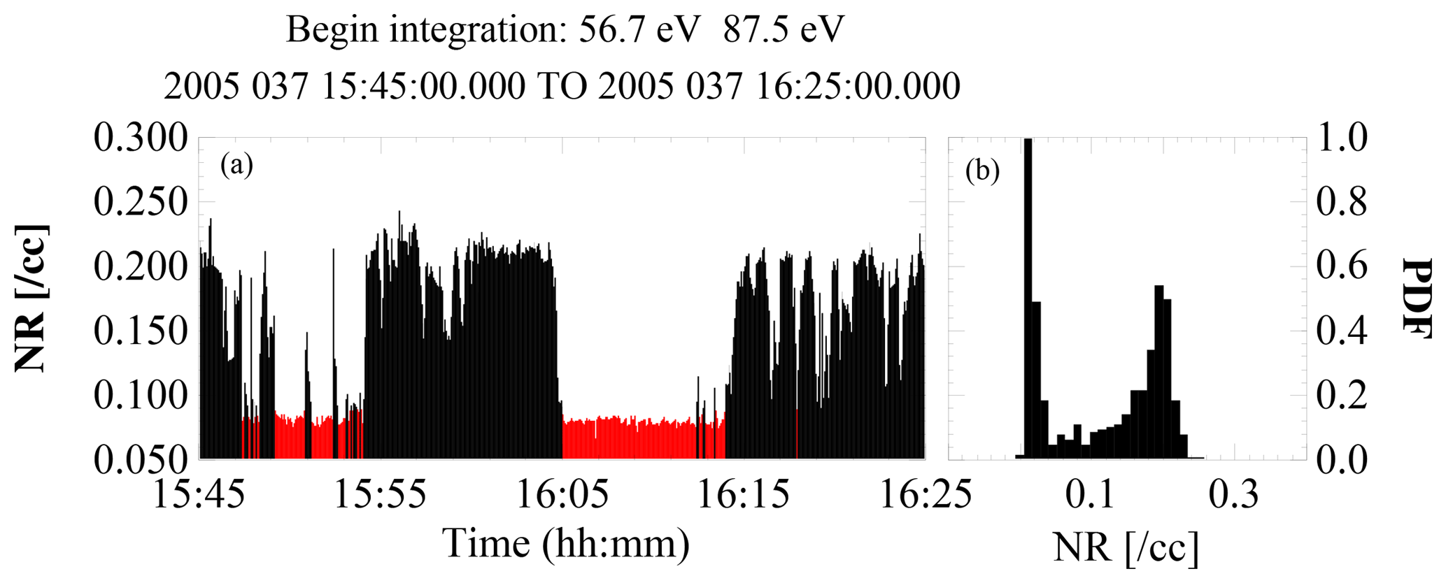
Figure 2Figure demonstrates the bimodal aspect of the return electron density upstream of the bow shock. Panel (b) is a PDF computed for a 40 min stretch when Cluster-2 was upstream of the shock. The two bimodal peaks are obvious. Panel (a) shows the time dependence of the same data. Red indicates when the spacecraft was in the solar wind, which was determined using a 0.09 cm−3 breakpoint in the return density.
4.2 Shock normal
Analytically deriving either the expected pitch-angle spread of the return distribution or the expected energy gain in the reflection process requires an estimate of the shock normal. In this study we use the method described in Shen et al. (2007), which is based on the assumption that the shock normal is antiparallel to the gradient of the magnetic field within the shock front. Gurgiolo et al. (2005) described the multispacecraft methods for computing vector field gradients (curls, vorticity and divergence). Here we implement that approach using 5 vector per second FGM magnetometer field data from the four spacecraft. The result of the analysis is an estimate of the normal vector (in component form in GSE coordinates) with a 1σ deviation given for each component. As with most of the results described in this paper, the method is only valid when the four Cluster spacecraft are in a good tetrahedral configuration (Robert et al., 1998).
4.3 Energization through reflection
To make direct comparisons between the return and strahl populations, it is necessary to remap the return electrons in energy to account for any energy gained in the reflection process. For example, if the energization on reflection is a factor of 2 then the strahl density above ϵ eV should be compared to the return density above 2ϵ eV. The energization can be estimated using the methods described in Sonnerup (1969); Paschmann et al. (1980) to compute the ratio of reflected and incident energies. To implement this method one only needs the direction of the shock normal, as obtained using the Shen et al. (2007) technique. Assuming that the reflected electrons are associated with the strahl, which is either parallel or antiparallel to the magnetic field, knowing the shock normal allows one to estimate the energization directly using Paschmann et al. (1980) Eq. (9). We computed the energization for a number of shock normals and upstream magnetic field orientations by varying the shock normal direction and the magnetic field direction within a 1σ band about their measured component values.
4.4 Estimated pitch-angle spread of the reflected electrons
Under the assumption that the shock is a solid reflective surface, that all reflections are specular, and that the incident strahl guiding center velocity is parallel or antiparallel to the average magnetic field (depending on whether it is pointing sunward or antisunward), it is possible to estimate the pitch-angle spread (over the 4 s spin period) expected of the return electron distribution. The width is estimated by varying both the shock normal and average magnetic field components within their 1σ bands (as done when estimating the energization in reflection) coupled with a spread in the incident strahl velocity determined from its maximum pitch-angle spread as obtained using the ϕ–θ plots (viz., black outline in the first column of plot in Fig. 1). The estimates of the return pitch-angle spread can at times be a bit high when compared to what is observed in the ϕ–θ plots because we use a strahl pitch-angle limit that is generally on the high side to ensure that the total distribution is included in the limits.
4.5 Crossover energy
In both the solar wind and the foreshock there is often an energy below which the strahl begins to overlap the core–halo and the two populations cannot easily be separated, which we refer to as the crossover energy. Although rarely needed, it is possible to define a crossover energy for the return and core–halo populations. The crossover energy (or sometimes the energy above it) defines the starting energy used in the plasma moment integrations of the isolated populations. In the ϕ–θ plots the crossover energy is characterized by a shift in the population location in the plot. Above the crossover energy, the population is predominantly field aligned and the strahl is by far the dominant population, while below the cutoff energy the core–halo is dominant and the population shifts to a more radial profile. This is present in all of the upstream eVDFs, except at times when there is sufficient separation between the two populations, so that no crossover energy exists (both populations are fully separable at all energies). The crossover energy may vary from event to event and even within an event with major changes of the magnetic field orientation. For the most part, however, the crossover energy remains reasonably constant within a given event. At times when the interplanetary magnetic field is basically radial, the crossover energy is not easily identifiable and can be difficult to identify when the field has only a small nonradial component. In most cases, however, the energy at which the shift in dominance between the two populations occurs is unmistakable. The case seen in Fig. 1 is a situation in which the magnetic field has only minor nonradial components, making it difficult to identify the crossover energy, which we estimate to be close to 56.7 or 48.9 eV, where the strahl begins to extend toward lower θ.
4.6 Common figure formats
We basically use three figure formats to illustrate the plasma characteristics of each of the selected events. These consist of an event overview, a set of ϕ–θ plots illustrating the characteristics of a typical foreshock eVDF during the event, and a plot showing the densities of the total, return, and strahl populations across the time period. All figures of one type share a common format.
-
The overview figure (e.g., Fig. 3) consists of two panels. The upper panel is the full electron density and total fluid velocity with density plotted against the left axis and velocity against the right axis. Below this is a spectrogram from the PEACE elevation that is closest to the ecliptic overlaid with a plot of the magnetic field. All data are plotted at 4 s resolution. Higher-resolution magnetic field data are included in plots in the discussion section.
-
The characterization of a typical eVDF from the foreshock for the event is shown in a set of three columns of ϕ–θ plots (e.g., Fig. 4). These form a set of 18 contiguous (in energy) ϕ–θ plots, which together cover the energy range from 15.8 to 669.2 eV. White and red traces in each plot are lines of constant pitch angle and are basically included to delineate where, if present in the plots, the strahl (white) and return electron distributions (red) are expected to be observed. These are also the same regions used to isolate the two populations in the estimation of their plasma moments (viz., Fig. 1). The solid dot and triangle in each plot are the projections of the head and tail of the magnetic field. The plots have no smoothing applied to them and display the data in their native ϕ–θ resolution.
-
The density information figure (e.g., Fig. 6) contains two columns, each consisting of four rows of plots. From top to bottom these are the full, strahl, and return densities and the return-to-strahl density ratio across the event. The left-hand column of plots shows the time variation of the quantities, while the right-hand column consists of plots of the probability density function (PDF) of the quantities from just the foreshock periods. The average values of the plotted quantities for both regions are shown to the right of each PDF plot (foreshock, black text and solar wind, red text). If one or the other of the regions is not sampled in the event, the average value is set to −1.0. In the lower three panels of plots in the first column the red portion(s) of the plot indicate times when the spacecraft are in the solar wind and the black portions indicate times when the spacecraft is in the foreshock. This is determined directly from the return electron density as discussed in Sect. 4.1.
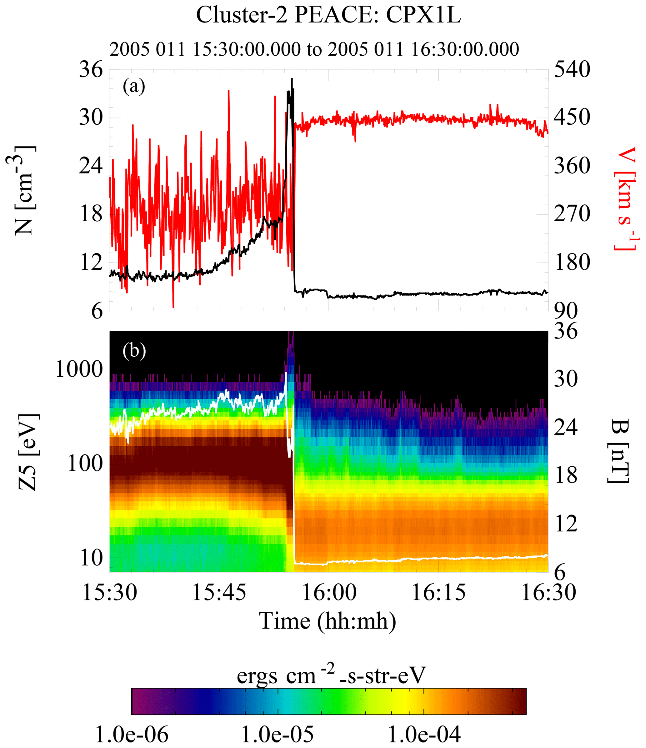
Figure 3An overview of the 11 January 2005 event. Panel (b) shows an energy spectrogram of the electron data from one of the near ecliptic heads of PEACE overlaid by a trace of the magnetic field (white). Panel (a) contains the full electron density (black) and the bulk fluid velocity (red). All data were from C2. At 15:55 the spacecraft exits the magnetosheath, passes through the bow shock, and enters the upstream solar wind. For about the first minute the spacecraft is in the foreshock and then transitions into the solar wind, staying there for most of the remaining time period.
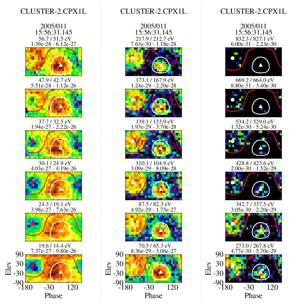
Figure 4A set of ϕ–θ plots showing each energy step from 15.8 to 669.2 eV from a single eVDF in the foreshock. The white and red traces are lines of constant pitch angles (120 and 75∘) and are shown solely to indicate the areas where the strahl (white) and return electrons (red) might be expected to be found. The presence of either population may not exist at any given energy.
Although we have looked at multiple events as part of this study, we present the detailed results for only three. These are typical and illustrate most of the important features pertinent to this analysis.
5.1 Event 1: 11 January 2005
Figure 3 is the event 1 overview. All data were obtained from C2. The event begins in the magnetosheath and at about 15:55 UT the spacecraft passes through the bow shock and enters the foreshock. There is only a short stretch of foreshock (about 45 s) before the spacecraft crosses into the solar wind and remains there for most of the rest of the event with the last 90 s spent in the foreshock. This is explicitly shown in Fig. 6.
Figure 4 shows a partial representation of a typical foreshock eVDF observed just after the spacecraft crosses the bow shock. Both the strahl and return electron distributions are field aligned and counter-streaming, the strahl is moving antisunward and the return electrons are moving sunward. The white and red traces in each plot are lines of constant pitch angles of 120∘ (≡60∘) and 75∘. The region delimited by the white trace marks the strahl and the region delimited by the red trace marks the return population. Neither population needs to be present at any given energy.
In this event the crossover energy is located at about 56.7 eV. Above this energy the electron distribution consists almost exclusively of strahl and return particles. Below this energy there is an obvious contribution of core–halo electrons that rapidly becomes the dominant population. There is still a return electron signature below the crossover energy, probably extending to as low as 37.7 eV. The return electrons are noticeably nongyrotropic at the lower energies, particularly below the crossover energy, where they appear as a partial ring, probably as the result of a combination of phase bunching in the reflection process and subsequent gyrophase mixing and possibly phase locking. As we demonstrate below, it appears that above the crossover energy all of the return electrons originate from the strahl. At lower energies the return electron signature is more likely due to reflection of some percentage of the higher energy halo electrons together with some lower-energy strahl that is not fully separable from the core–halo. In the ϕ–θ plots the core–halo population (when present) is centered near (0∘, 0∘) because it flows radially outward from the Sun. (Recall that the spacecraft spin axis is not quite perpendicular to the ecliptic plane.) Halo and strahl electrons that overlap in velocity space will react identically to any external influences.
The angular spread observed in the return electrons in the ϕ–θ plots appears to be consistent with specular or nearly specular reflection. Computation of the shock normal returns a vector of 0.780±0.033, 0.603±0.043, 0.121±0.098 in GSE coordinates, which when coupled with the average magnetic field just upstream of the shock in the foreshock gives a of 81∘. Assuming a maximum spread in the strahl pitch angle of 60∘, we estimate there should be an 81±5∘ spread in the return electron pitch-angle distribution. The best fit to the return data as determined from the ϕ–θ plots would appear to be a spread of about 75∘ (red trace in Fig. 4).
Above the crossover energy, the return distribution almost exactly matches the energy range covered by the strahl electrons, extending one or two energy steps higher to energies where there is no evidence of strahl. At these energies the weak count rate has the appearance of noise and, were it not for the fact that it is observed exclusively within the region in phase space associated with the return distribution, it would probably be labeled as such. The higher energy is in all likelihood the manifestation of acceleration in the reflection. That acceleration would put the source of the return electrons below the crossover energy, directly within the upper halo.
Using an ensemble of energizations obtained from Eq. (9) in Paschmann et al. (1980), we place the average energization factor in the reflection process at 1.17. Figure 5 shows the results as a PDF plot. This value can be used to remap the return electron densities for comparison with the strahl. Under the assumption that above the crossover energy the observed reflected population has the strahl as its source, we compared the estimated strahl density with energies ≧70.5 eV with that of the return densities with energies ≧87.5 eV (87.5 eV being the closest center energy being returned to eV). We did this by computing the strahl and return densities within each returned energy band and then summing the densities over the energies ≧70.5 eV for the strahl and ≧87.5 for the return electrons. This mapping is equivalent to an energization factor of 1.24. The results are shown in Fig. 6, beginning from just after the shock crossing to 16:30 UT. For this energization mapping, the ratio of return to strahl electrons is 1.04. This was unexpected as the implication is that at least above 70.5 eV there is statistically a full reflection of the strahl at the shock. As a check we increased the starting energies of the density summation up one energy bin for both the strahl and return populations (to 87.5 eV for the strahl and to 110.1 eV for the return electrons, which corresponds to an the energization of 1.26), giving an average density ratio of 1.01.
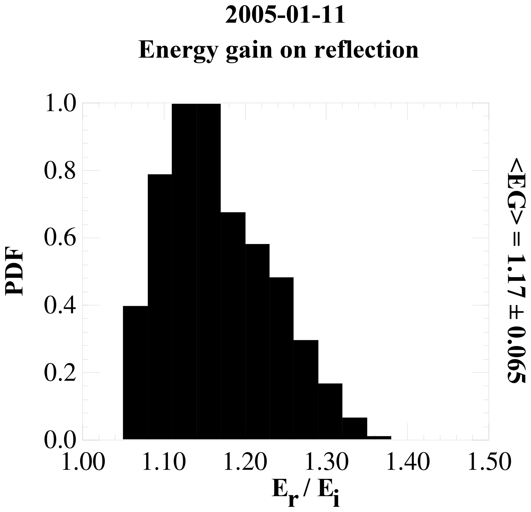
Figure 5PDF plot of the energy gain on reflection from the bow shock. The PDF was formed from the results of the energization model by varying the shock normal and magnetic field components within a 1σ band about their average values. The average energization and the 1σ value are shown to the right of the plot.
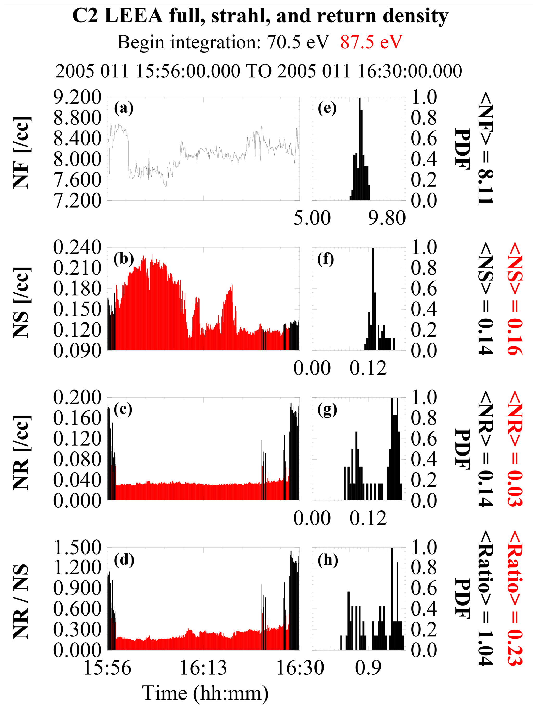
Figure 6Electron density information across the 11 January 2005 event. From top to bottom, the total, strahl, and return electron densities and the ratio of the return to strahl density across the event. Panels (a–d) show the values as a function of time. The red portions in (b–d) show when the spacecraft was in the solar wind. Panels (e–h) are the corresponding PDF plots of the foreshock density only. The average foreshock and solar wind densities are shown to the right of each PDF plot (red solar wind, black foreshock). The beginning energy integration used to estimate the density in each region is shown at the top.
5.2 Event 2: 6 February 2005
Figure 7 shows the overview of event 2. As in the previous event, the spacecraft begins in the magnetosheath and a little before 15:45 UT passes through the bow shock and into the foreshock, where it stays for a little longer than 2 min before entering the solar wind. There are multiple excursions into and out of the foreshock at this point over the rest of the event. Overall the spacecraft spends a significantly larger percentage of time in the foreshock than it did in the previous event, which improves the statistics in the observed return-to-strahl density ratio, as is readily apparent in Fig. 9.
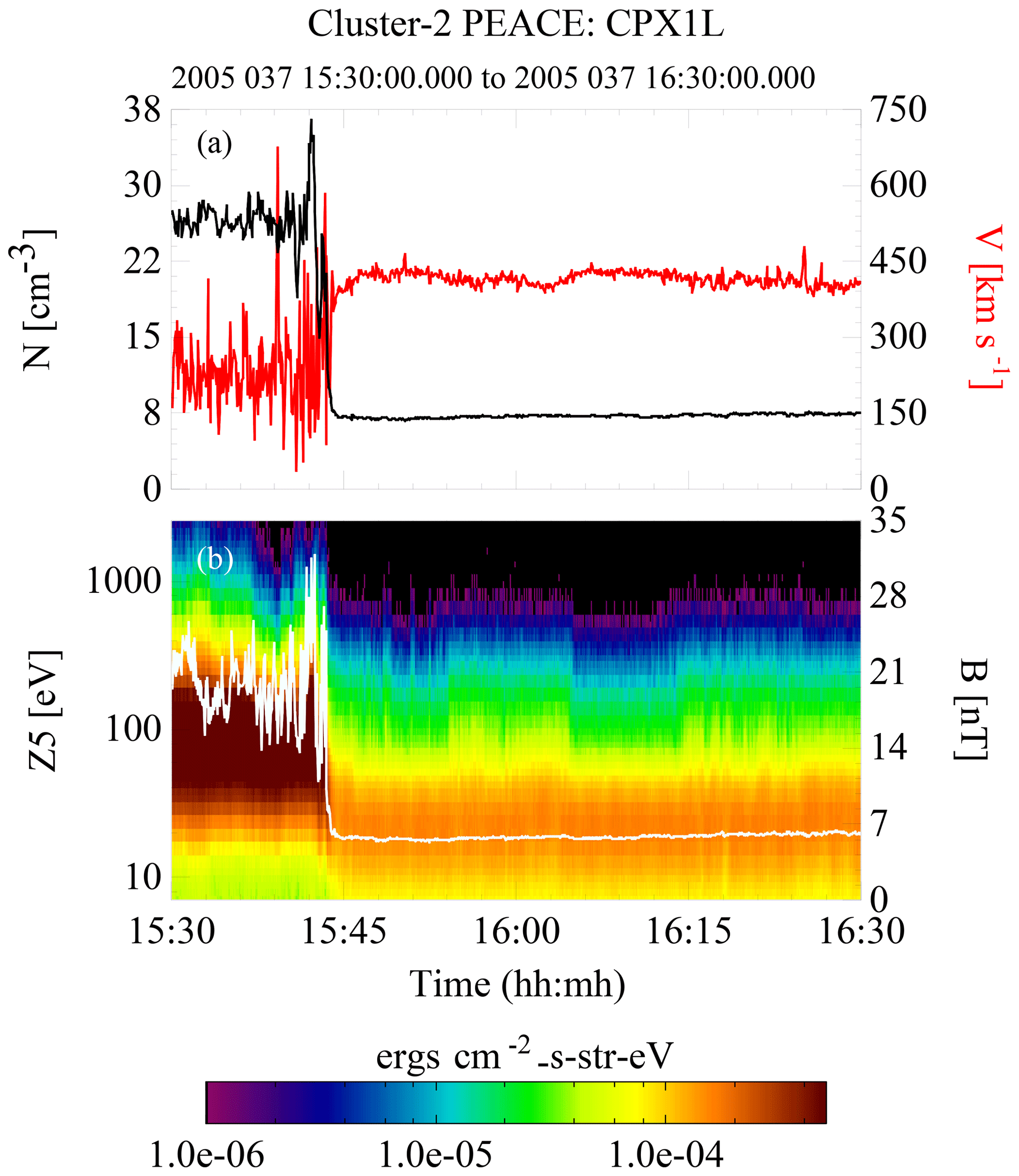
Figure 7An overview of the 6 February 2005 event. Panel (b) shows an energy spectrogram of the electron data from one of the near ecliptic heads of PEACE overlaid by a trace of the magnetic field (white). Panel (a) contains the full electron density (black) and the bulk fluid velocity (red). All data were from C2. At 15:45 the spacecraft exits the magnetosheath, passes through the bow shock, and enters the upstream solar wind. For about 2 min the spacecraft is in the foreshock and then transitions into the solar wind. There are two major periods of solar wind before the end of the event that can be seen in Fig. 10.
The spacecraft were in a good tetrahedral configuration during this event and the shock normal was estimated to be 0.692±0.025, 0.161±0.007, 0.703±0.027 in GSE coordinates. The average magnetic field just upstream of the shock gave a of 70∘. Using a 50∘ pitch-angle spread for the strahl we obtained an estimate of the pitch-angle spread for the return electrons of 74±5∘. The pitch-angle spread determined directly from the ϕ–θ plots in Fig. 8 was 75∘ (the red trace). The white trace used to delineate the strahl is a pitch angle of 50∘.
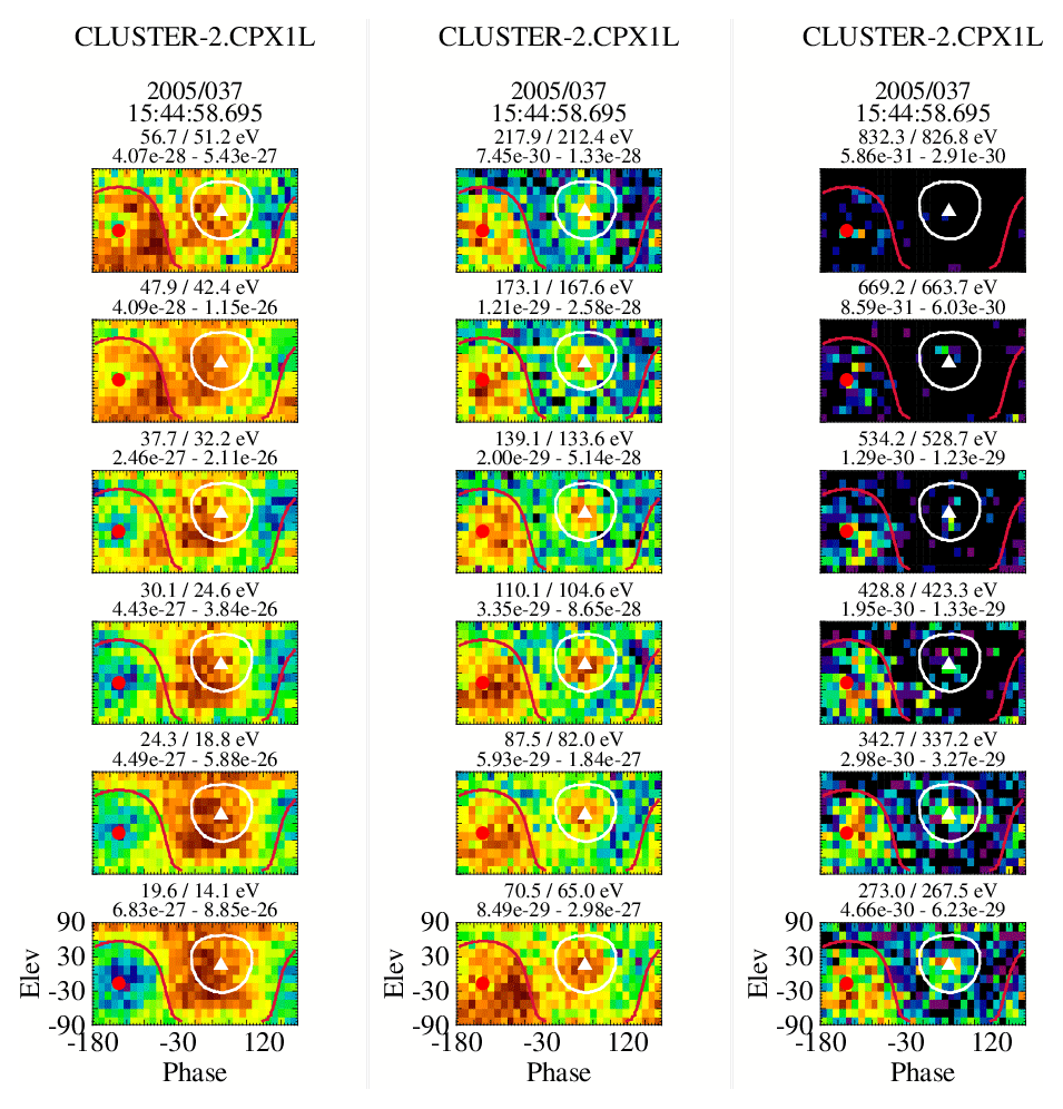
Figure 8A set of ϕ–θ plots showing each energy step from 15.8 to 669.2 eV from a single eVDF in the foreshock. The white and red traces are lines of constant pitch angles (130 and 75∘) and are shown solely to indicate the areas where the strahl (red) and return electrons (white) might be expected to be found. The presence of either population may not exist at any given energy. The solid triangle and dot in the plots are the projections of the tail and head of the magnetic field vectors.
Comparing Fig. 4 with Fig. 8 shows only minor differences in the eVDF morphology between the two events. The crossover energy is, however, slightly lower in this event, probably 47.9 eV. The return electron signature again extends below the crossover energy down to at least 37.7 eV and is distinctly nongyrotropic at the lower-energy end.
As shown in Fig. 9, the energization factor associated with this shock is estimated to be 1.43. Figure 10 shows the electron density profiles of the different populations across Fig. 7, starting just after the spacecraft exits the bow shock. In the plot, the strahl density was determined, beginning from 56.7 eV, and the return density began from 87.5 eV. This mapping accounts for an energization factor of about 1.54, which is slightly larger than the analytical estimate. The ratio (1.01) implies that there is full reflection of the strahl in this event, at least for this mapping. We looked at two further energy ranges with the strahl density summation beginning at energies 70.5 and 110.1 eV and return density beginning at 87.7 and 139.1 eV (both essentially having mappings equivalent to an energization factor of about 1.57). These give return-to-strahl density ratios of 1.08 and 1.05.
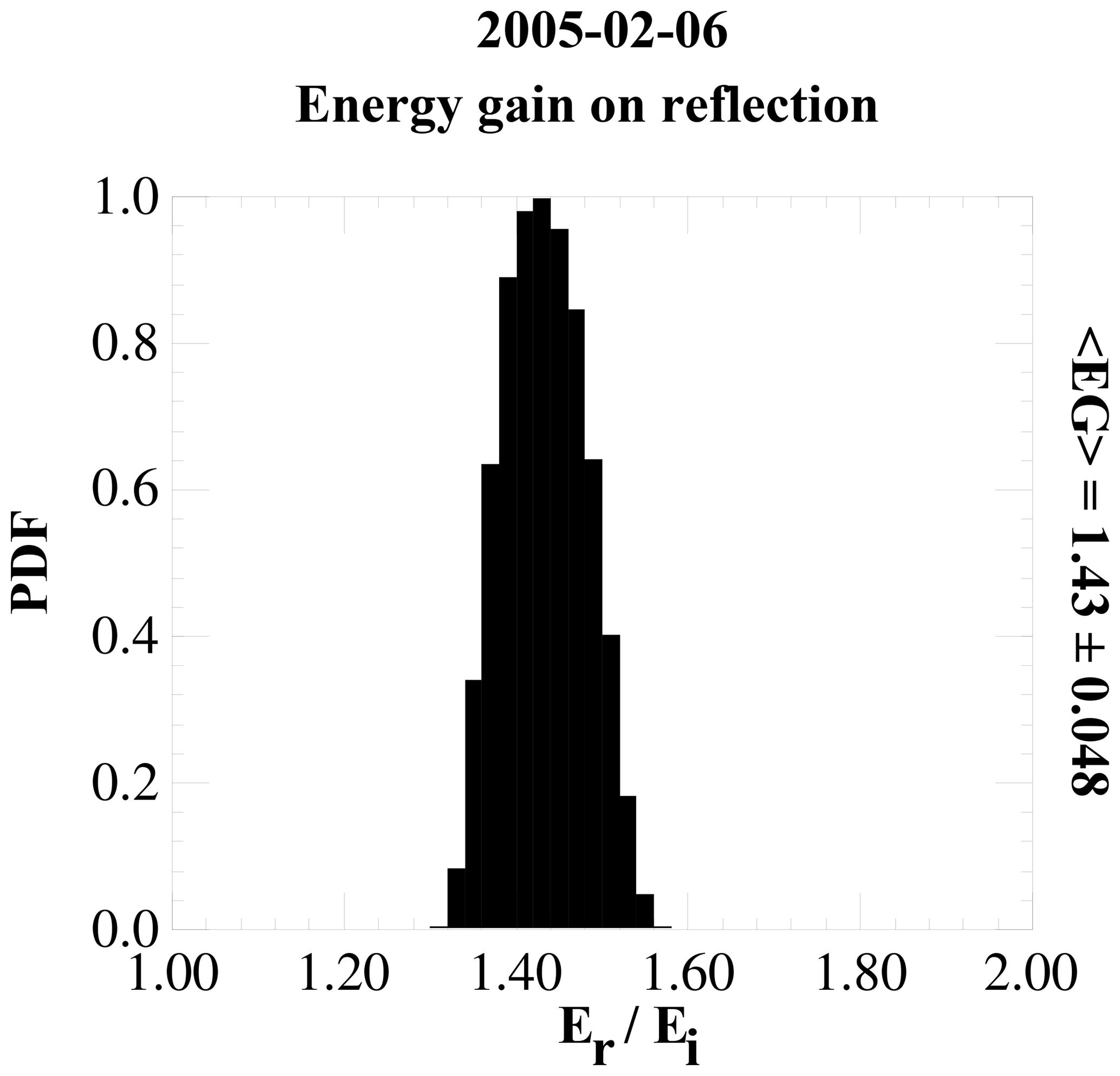
Figure 9PDF plot of the energy gain on reflection from the bow shock. The PDF was formed from the results of the energization model by varying the shock normal and magnetic field components within a 1σ band about their average values. The average energization and the 1σ value are shown to the right of the plot.
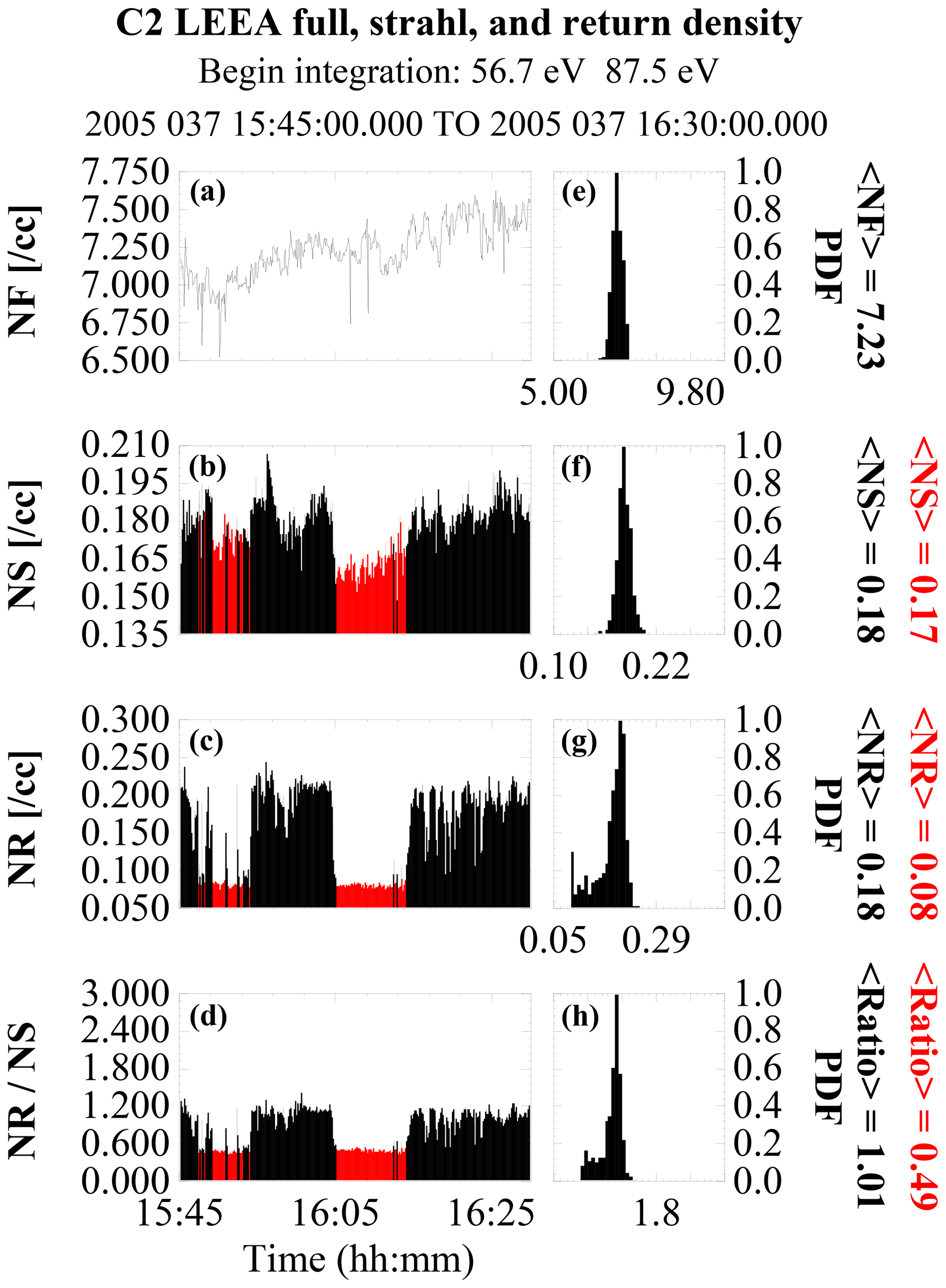
Figure 10Electron density information across the 6 February 2005 event. From top to bottom are the total, strahl, and return electron densities and the ratio of the return to strahl density across the event. Panels (a–d) show the values as a function of time. The red portions in (b–d) show when the spacecraft was in the solar wind. Panels (e–h) are the corresponding PDF plots of the foreshock density only. The average foreshock and solar wind densities are shown to the right of each PDF plot (red solar wind, black foreshock). The beginning energy integration used to estimate the density in each region is shown at the top.
5.3 Event 3: 15 April 2008
The overview of the third event is shown in Fig. 11. Again, the event begins in the magnetosheath with a bow shock crossing at about 19:15 UT. The spacecraft then enters the region upstream of the foreshock (Fig. 13) and remains there for the rest of the event, with the exception of a short excursion into and out of the solar wind near 19:28 UT. Unfortunately, for this event the four spacecraft were not in a good tetrahedral configuration and no estimate of the shock normal was possible. But an estimate of the shock normal is not critical for this event, as we have demonstrated in the first two events that the analytically derived values of both the angular width of the return distribution and the reflection energization factor closely match what can be obtained directly from the data.

Figure 11An overview of the 15 April 2008 event. Panel (b) shows an energy spectrogram of electron data from one of the near-ecliptic sensors of PEACE overlaid on a trace of the magnetic field (white). Panel (a) contains the full electron density (black) and the bulk fluid velocity (red). All data were acquired from C2. At about 09:15 UT the spacecraft exits the magnetosheath, passes through the bow shock, and enters the upstream region and is in the foreshock for the remaining time period, with the exception of a brief excursion into the solar wind at about 19:28 UT.
For this event we obtained a pitch-angle spread of 70∘ for the return electrons directly from the ϕ–θ plots (Fig. 12) and estimated the reflection energization factor from plots of the density ratio constructed with varying starting integration energies of both the strahl and return populations to be on the order of 1.58. Figure 13 shows the population densities and density ratio constructed with the strahl and return densities beginning at 110.1 eV and 173.1 eV, respectively. This is equivalent to a 1.57 energization factor and gives a density ratio of 0.99. Lowering the beginning energy step in the estimation of both densities to 87.5 and 139.1 eV (equivalent to a reflection energization factor of 1.59) changes the average ratio to about 1.01. Lowering the starting energy of the two populations one energy step further (equivalent to a reflection energization factor of 1.56) increases the density ratio to about 1.1.
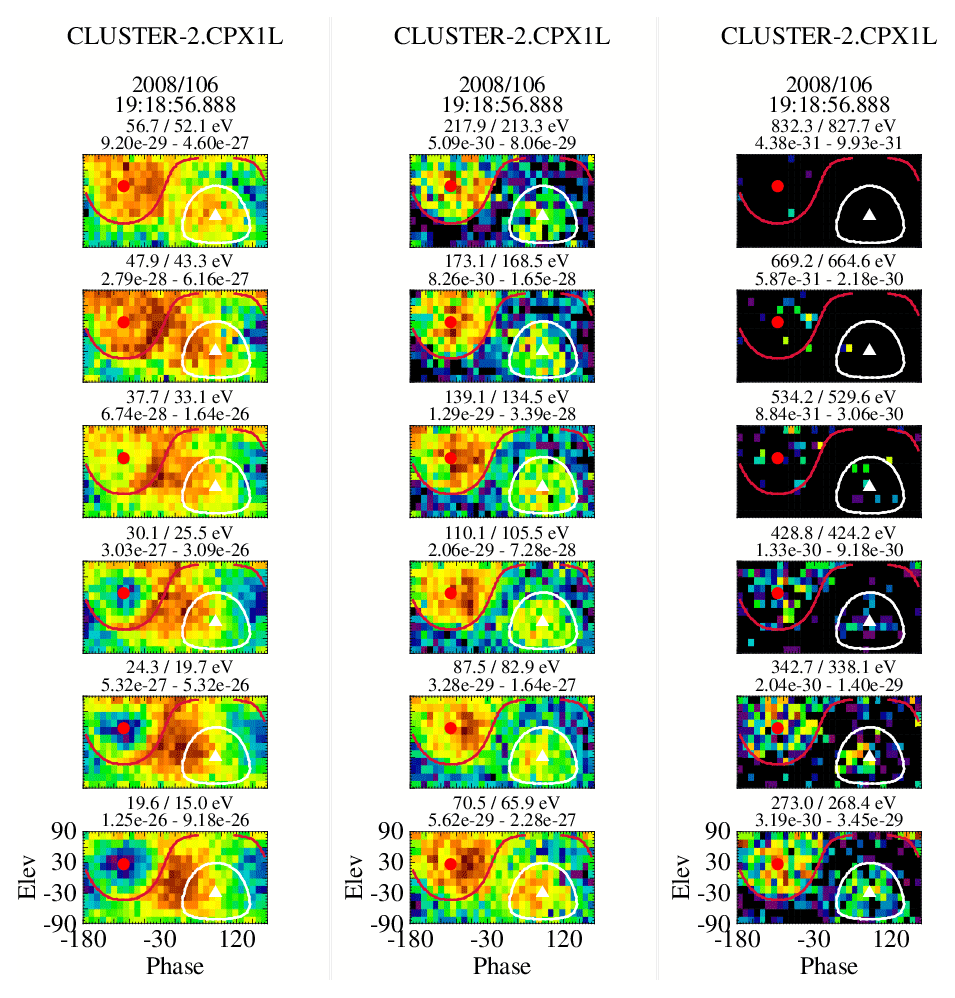
Figure 12A set of ϕ–θ plots showing each energy step from 15.8 to 669.2 eV from a single eVDF in the foreshock. The white and red traces are lines of constant pitch angles (125 and 70∘) and are shown solely to indicate the areas where the strahl (white) and return electrons (red) might be expected to be found. The presence of either population may not exist at any given energy. The solid triangle and dot in the plots are the projections of the tail and head of the magnetic field vector.
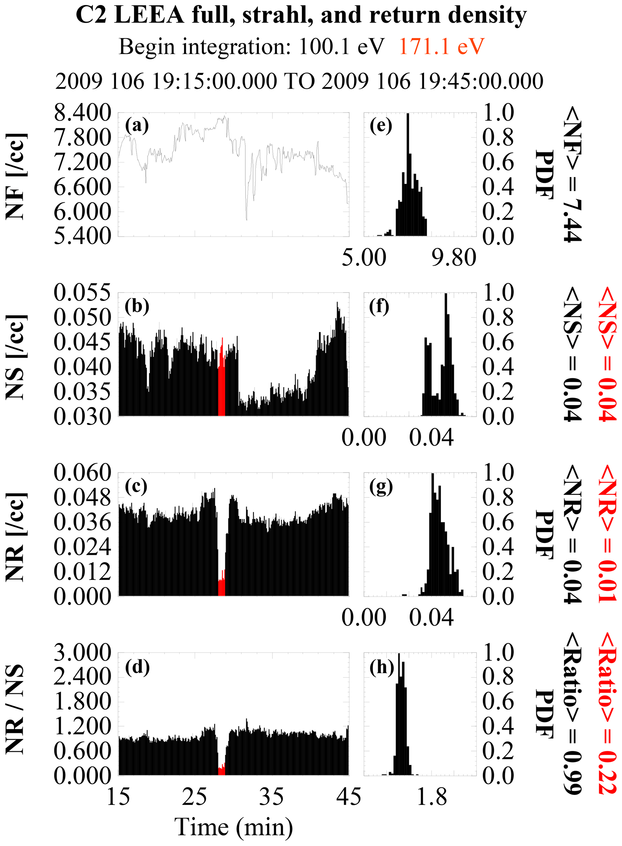
Figure 13Electron density information across the 15 April 2008 event. From top to bottom, the total, strahl, and return electron densities and the ratio of the return to strahl density across the event. Panels (a–d) show the values as a function of time. The red portions in (b–d) show when the spacecraft was in the solar wind. Panels (e–h) are the corresponding PDF plots of the foreshock density only. The average foreshock and solar wind densities are shown to the right of each PDF plot (red solar wind, black foreshock). The beginning energy integration used to estimate the density in each region is shown at the top.
5.4 Errors
There are several recognized sources of error that can affect portions of the event analysis, in particular, the comparisons of the strahl and return densities. Primary among these possible errors is the analytical estimate of the reflection energization factor. The error is purely statistical, resulting from the use of all possible combinations of magnetic field and normal orientations within the 1σ band about the actual component measurements. This value determines the remapping in energy of the return population. As can be seen from Figs. 5 and 9, the error is not large, but even small errors can significantly affect the estimation of the measured return-to-strahl density ratio, which depends on the ability to remap the return density in energy. The remapping often splits the starting energy between two energy bins. Depending on which starting point energy is selected in summing up the density moment, one will either over- or underestimate the return density, and that factors into the average return-to-strahl density ratio. Another statistical error arises when the spacecraft spends insufficient time in the foreshock to amass a good statistical number for the average return densities. Such errors give rise to an overall larger standard deviation in the density ratio. A final source of error that can affect the density ratio arises when only a single estimate of the energization factor per event is obtained at the shock crossing. Changes in the orientation of both the shock normal and upstream magnetic field over the course of an event in reality will continuously change the energization. The remapping used to mesh the return and strahl density estimates is unlikely to remain constant across the event as we currently assume.
Unlike the solar wind, the foreshock is a region characterized by large amplitude waves and turbulence, which arises, in part, from backstreaming ions and electrons created from the reflection of the incident solar wind off the shock. Both populations are field aligned and together they provide the necessary free energy to drive a number of instabilities which, for example, can generate MHD and ULF waves along with Langmuir waves. The instabilities are responsible for the initial scattering and preheating of the solar wind as it approaches the shock.
Ion reflection off the shock is better understood than that of electrons, primarily because it has been studied in greater detail. Simulations have played a substantial role by providing a large number of possible reflection mechanisms, but the simulations have not provided information as to which mechanism(s) are dominant or most important. The results of this study indicate that the reflected electrons are primarily the strahl electrons, which may place limits on some of the available reflection mechanisms. Like the ions, the electrons gain energy in the reflection, as can be seen at the upper-energy ϕ–θ plots in Figs. 4, 8, and 12. Although the counts are weak in these plots, it is obvious that the return electrons extend a few energy bands higher than the strahl due to energy gained in the reflection process.
The increase in angular width of the return electrons over the incident strahl is consistent with a specular reflection. The same is true of the formation of the partial ring distributions often observed in the lower-energy ϕ–θ plots (cf. the top three plots in the first column of Fig. 8). This is probably the result of gyrophase bunching in the reflection process and, if observed far enough upstream, would imply the presence of an active-phase trapping mechanism (Gurgiolo et al., 2000, 2005). Electrons phase-mix extremely rapidly and, coupled with their higher speed, should isotropize significantly closer to the bow shock than do the ions.
While the ratio of the incident and reflected population densities is highly suggestive of a full reflection of the strahl, at least above the crossover energy, there are other indications that lead to the same conclusion and provide even more information about the process. Two of the more obvious questions that can be addressed include “where does the reflection occur?” and “how thick is the reflecting region?” Answering both questions can be approached by using a series of ϕ–θ plots to monitor the strahl as it approaches the bow shock and observe the changes that occur in the eVDFs.
From an idealistic observational point of view, if there is a full reflection of the strahl one might expect that at some point both it and the return electron population would just drop out of the ϕ–θ plots. Where this occurs would then be the reflection point. If the reflection were sufficiently rapid, occurring within one or two gyroradii, given the spacecraft velocity and the cadence of 3-D eVDFs being returned, the reflection would appear from the PEACE data to be almost instantaneous. On the other hand the strahl might be observed to gradually weaken until it is no longer a significant population. The time over which that occurred would represent the thickness of the reflection region.
There are drawbacks to this approach. If there is no full reflection of the strahl, then some fraction of it will penetrate into the downstream region, but the return population should still vanish in the ϕ–θ plots after the reflection point. The problem is that it is not obvious that it does. No matter whether the strahl is fully or partially reflected, there will always be a plasma presence downstream of the reflection point and this plasma will, regardless of its source, either be field aligned or moving radially with the solar wind. Any other flows require the identification of additional forces such as might be provided by the cross shock potential. The problem becomes how to determine whether populations seen downstream of the reflection point are the same as or different from the populations seen upstream of the reflection point, in particular, the return electrons.
As there is no guidance on how to differentiate field-aligned electrons downstream of the reflection point from the return electrons upstream of the reflection point, we developed a basic set of criteria to use to accomplish this. The criteria stipulate that, once it is obvious that the reflection point has been crossed, an observed population might be a signature of the reflected strahl if the following conditions apply:
-
The population in question is field aligned and moving back into the upstream.
-
The population covers approximately the same energy range as the return electrons upstream of the reflection point.
-
The population has roughly the same angular spread as the return electrons upstream of the reflection point.
-
The population is approximately continuous in time, i.e., not intermittent.
The result of this type of analysis is shown in Fig. 14, which contains a column of three spectrograms from PEACE elevation zone 5 (near ecliptic view), with one plot corresponding to each of the three analyzed events. Each spectrogram is overlaid by the local magnetic field. These convey similar information to that shown in Figs. 3, 7, and 11 but only cover about 2 to 3 min about the shock crossings to provide for a higher-resolution view. The PEACE spectra have been spin averaged and the magnetic field has a 0.2 s temporal resolution. In each plot the foot of the shock and shock ramp are clear.
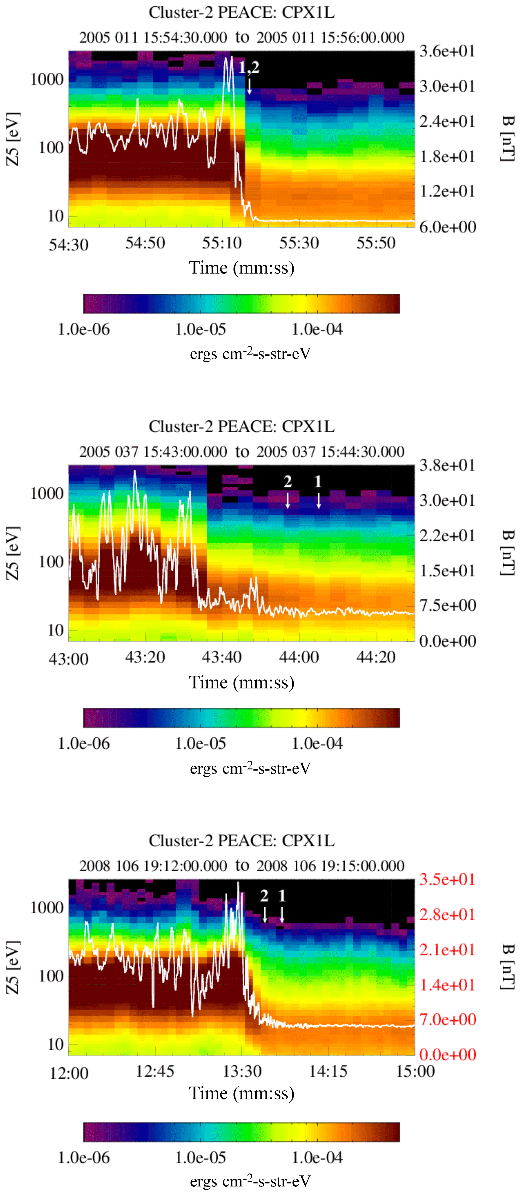
Figure 14High-resolution plots of the shock crossings for each of the three events. Each plot contains a spectrogram of the PEACE elevation Zone 5 sensor overlaid by the magnetic field. The spectrogram has a one-spin resolution and the magnetic field resolution is 0.2 s. There are two numbered arrows in each plot. Arrow 1 is the point at which the strahl disappears from the ϕ–θ plots and arrow 2 is where the return electron signature disappears. The location of the arrows is somewhat subjective, especially for arrow 2.
Each crossing has associated with it a pair of arrows labeled 1 and 2. The position of arrow 2 marks what can be thought of as the most forward boundary of the foreshock as it nears the shock. It is the time of the last unequivocal observation of an electron eVDF that contains both return and strahl populations. At times earlier than arrow 2, there is no observable strahl signature in the ϕ–θ plots, the implication being that arrow 2 marks the location of the reflection point. The absence of the strahl before the reflection point suggests that the strahl could be fully reflected. There is, however, a return electron signature at and after the time of arrow 1. The return population is either absent or unobservable at earlier times. It should be emphasized that the locations of these arrows are somewhat subjective (arrow 1 much more so than arrow 2).
We are reasonably certain of the placement of arrow 2 in all of the plots (it is obvious when the strahl drops out of the ϕ–θ plots); the location of arrow 1 is more problematic. This arises from the identification of electrons observed prior to arrow 2. We use the 6 February 2005 event to illustrate the problem. Figure 15 contains seven time sequential columns of ϕ–θ plots, each characterizing an eVDF at seven energy steps between 30.1 and 342.7 eV. The energy steps are not sequential but chosen to give the best overall view of where changes on the eVDF are occurring. The figure covers the time frame between 15:43:40.6 and 15:44:05 UT, which includes both arrows in the middle plot in Fig. 14. The time of arrow 2 is covered in the seventh column and the time of arrow 1 is covered in the fifth column. The first sweep in each plot is against the left-hand axis, which marks the starting time.
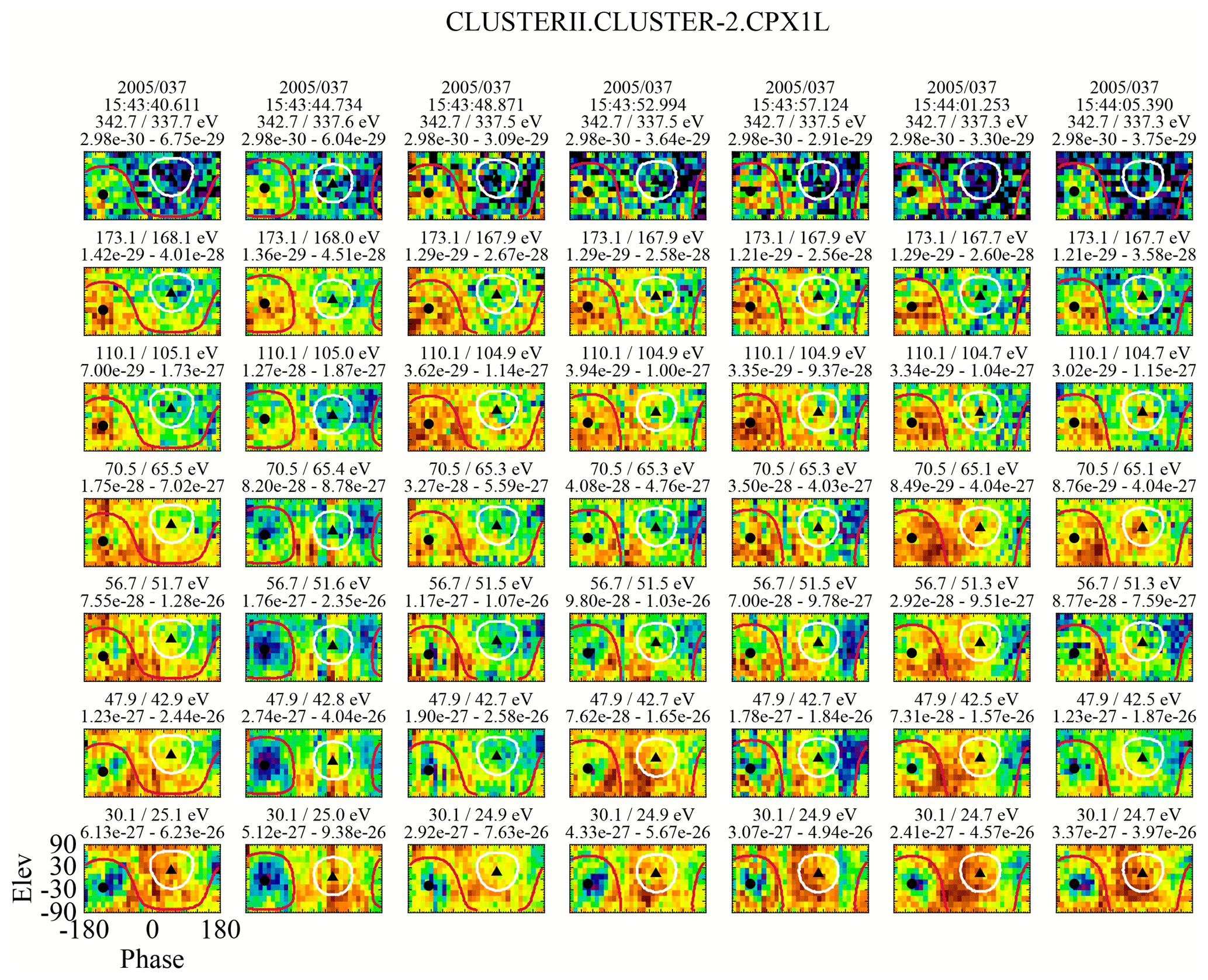
Figure 15Characteristics of seven sequential eVDFs shown through ϕ–θ plots, which span the arrows shown in the center plot of Fig. 14. Recall that the location of the strahl, when present, is expected within the white circle, while the return electrons are expected within the red circle.
Column 7 in the figure is unquestionably from the foreshock as it exhibits both a return and strahl signature down to at least 70.5 eV. The crossover energy is at 56.7 eV, and below this there is just a core–halo and a return population signature. The return electrons are anisotropic at the lower energies and that may extend to energies above, where it is seen farther upstream (e.g., Fig. 8). This perhaps is to be expected so close to the reflection point but other than this there is little difference between what is observed in column 7 from what is seen in the eVDFs that follow it in time (not shown). The eVDF in column 6 is very similar to that in column 7 but with a weaker and less defined strahl signature and could probably represent the last foreshock eVDF as well as that of column 7, indicating that the reflection occurs in a very narrow transition region.
The first five columns show no evidence of a strahl population. There is, however, an electron presence within the strahl mask region, but this is more of a general background than a distinct population. The eVDFs do, however, show sunward-propagating field-aligned beam(s) that may or may not consist of reflected electrons. (Although, if they are reflected electrons, it is unclear what the incident particle population is.) One possibility would be that they are upper-energy halo electrons. Column 5 appears to be the first column of plots that shows a return electron distribution that is consistent with what is seen after it, although it is a bit weaker and less defined at the lower energies. The first four eVDFs contain backstreaming electron populations but with prominent and consistent deviations from what is seen in the last three columns of plots. There is, for example, no significant core–halo presence and at times (notably in the second column), no backstreaming electrons at the lower energies. The same features can be seen in earlier eVDFs (not shown here), but they are highly intermittent and exhibit considerable variation in energy and intensity, the latter peaking as would be expected with the increase in density at the shock. Observationally, we do not claim the presence of a return electron signature in the eVDFs as seen in the foreshock earlier than column 5. While this is subjective, it is probably not off by more than 4 s. Consequently, while Fig. 15 shows that arrow 2 in Fig. 14 is reasonably well placed, the placement of arrow 1 at 15:43:57 UT is less certain.
Even with the uncertainty in the placement of arrow 1 in the center plot of Fig. 14, it is clear that, contrary to the general descriptive phrase “reflection off the shock”, the reflection is actually occurring within the foot of the shock and not at, in, or behind the shock front itself. The same is true of the remaining two shock crossings in the figure, although the reflection in event 1 is very close to the ramp. These observations effectively rule out magnetic mirroring as a source of the reflection. First, because there is insufficient ΔB in the foot of the shock to account for any significant mirroring, and second, because there is no observed transition of any portion of the strahl into the region downstream of the reflection point. The strahl is reasonably field aligned, albeit with a 40 to 60∘ spread in pitch angle, which would preclude the mirroring of a significant percentage of the population. In each of the analyzed events, mirroring would not start until about a pitch angle of 40–50∘ (loss cone), which should leave the bulk of the strahl to penetrate downstream, which is not seen in the data. What exactly is causing the reflection at the foot of the shock is unclear. At least above the crossover energy, the reflection mechanism is very efficient.
Studies of the reflection of the ion solar wind have played a major role in our understanding, not only of the role of reflections in the physics associated with the foreshock, but also the physics of how the reflection occurs. However, some aspects of that process as gleaned from analyses of ion data may not apply to electrons. A major difference between the upstream features of electrons and ions comes from the strahl. Unlike the ions and the electron core–halo, both of which flow radially outward from the Sun, the strahl is field aligned. Except for times when the interplanetary field is highly radial, the reflection of the strahl need not mimic that of either the ions or of the core–halo. In this study we have found that the reflection of the electron solar wind appears to primarily consist of a reflection of the strahl and that, above a crossover energy, electrons appear to have been fully reflected in the foot of the shock as opposed to in the shock ramp where the magnetic mirror force would be expected to dominate. In the first event (top panel in Fig. 14) there is a small increase in near the breakpoint, but that is not the case in either of the other two events (middle and bottom panels in Fig. 14). Consequently, the details of precisely how the reflection occurs are not clear from this analysis, but it must primarily involve the field-aligned component of the distribution, viz., the strahl. One may have to study similar events with the higher-resolution data than is available from Cluster. Data from the Magnetospheric Multiscale mission may be useful in further elucidating the details of how the strahl is reflected in these quasi-perpendicular shock geometries. Based on the agreement between the observed spread in the return pitch angle with analytically produced spreads, we conclude that the reflection is specular. Below the breakpoint energy we cannot rule out a partial reflection of the upper-energy halo electrons or of strahl electrons, which may be mixed in with them. These two populations cannot be separated in our analysis at energies below the crossover energy.
The analysis and identification of just where the spacecraft were during the event was facilitated, in part, by the development of an algorithm that helped greatly in determining when the data came from when the spacecraft were in the foreshock as opposed to the solar wind. The basic assumption is that return electrons only exist in the foreshock. Consequently, when one sees a bimodal density pattern, the spacecraft is, perforce, in the foreshock. When the density is low and the pattern is not bimodal the spacecraft is in the solar wind and, conversely, when density is high (and bimodal), the spacecraft is in the foreshock. The pattern is shown in Fig. 2. Thus, an effective approach to separating the foreshock periods from solar wind periods is to set a breakpoint such that one is in the foreshock when the density is higher than that breakpoint, but in the solar wind when the density is below the breakpoint. The precise value of that breakpoint is not critical, as the examples we found indicate that the density values in the two modes are generally quite distinct.
Future studies using high-resolution data obtained in the foreshock should add to the number of events and help to determine precisely how solar wind electrons are reflected at Earth's bow shock.
All data are available from the Cluster Active Archive (https://csa.esac.esa.int/csa-web/; last access: 9 April 2019). This is a public repository of all the scientific data from the Cluster mission.
The authors declare that they have no conflict of interest.
The authors would like to acknowledge support from NASA through grant NNX15AI88G. The authors would also like to acknowledge the work and role of the Cluster Science Archive (CSA) in archiving and making available data from the Cluster mission. In addition, we also thank the WHISPER, EFW, FGM and PEACE teams for providing the data used in this study. In particular, we would like to thank the PEACE team at MSSL for their continued work in updating and improving the instrument calibration, especially for those data sets taken later in the mission.
This paper was edited by Christopher Owen and reviewed by two anonymous referees.
Anderson, K. A., Lin, R. P., Gurgiolo, C., Parks, G. K., Potter, D. W., Werden, S., and Rème, H.: A component of nongyrotropic (phase bunched) electrons upstream from the Earth's bow shock, J. Geophys. Res.-Atmos., 90, 10809, https://doi.org/10.1029/JA090iA11p10809, 1985. a
Bale, S. D., Burgess, D., Kellogg, P. J., Goetz, K., and Monson, S. J.: On the amplitude of intense Langmuir waves in the terrestrial electron foreshock, J. Geophys. Res.-Atmos., 102, 11281–11286, https://doi.org/10.1029/97JA00938, 1997. a
Balogh, A., Dunlop, M. W., Cowley, S. W. H., Southwood, D. J., Thomlinson, J. G., Glassmeier, K. H., Musmann, G., Luhr, H., Buchert, S., Acuna, M. H., Fairfield, D. H., Slavin, J. A., Riedler, W., Schwingenschuh, K., and Kivelson, M. G.: The Cluster Magnetic Field Investigation, Space Sci. Rev., 79, 65–91, https://doi.org/10.1023/A:1004970907748, 1997. a
Bonifazi, C. and Moreno, G.: Reflected and diffuse ions backstreaming from the earth's bow shock, 1, Basic Properties, J. Geophys. Res.-Atmos., 86, 4397–4413, 1981a. a
Bonifazi, C. and Moreno, G.: Reflected and diffuse ions backstreaming from the earth's bow shock, 2, Origin, J. Geophys. Res.–Atmos., 86, 4405–4414, https://doi.org/10.1029/JA086iA06p04405, 1981b. a
Burgess, D.: Simulations of backstreaming ion beams formed at oblique shocks by direct reflection, Ann. Geophys., 5, 133–145, 1987. a, b
Burgess, D. and Schwartz, S. J.: The dynamics and upstream distributions of ions reflected at the Earth's bow shock, J. Geophys. Res.-Atmos., 89, 7407–7422, 1984. a
Décréau, P. M. E., Fergeau, P., Krannosels'kikh, V., Leveque, M., Martin, P., Randriamboarison, O., Sene, F. X., Trotignon, J. G., Canu, P., and Mogensen, P. B.: Whisper, a Resonance Sounder and Wave Analyser: Performances and Perspectives for the Cluster Mission, Space Sci. Rev., 79, 157–193, https://doi.org/10.1023/A:1004931326404, 1997. a
Fazakerley, A. N., Lahiff, A. D., Wilson, R. J., Rozum, I., Anekallu, C., West, M., and Bacai, H.: PEACE Data in the Cluster Active Archive, The Cluster Active Archive, Studying the Earth's Space Plasma Environment, edited by: Laakso, H., Taylor, M. G. T. T., and Escoubet, C. P., Astrophysics Space, 11, 129–144, https://doi.org/10.1007/978-90-481-3499-1_8, 2010. a
Fitzenreiter, R. J., Viňas, A. F., Klimas, A. J., Lepping, R. P., Kaiser, M. L., and Onsager, T. G.: Wind observations of the electron foreshock, Geophys. Res. Lett., 23, 1235–1238, https://doi.org/10.1029/96GL00826, 1996. a
Fuselier, S. A. and Schmidt, W. K. H.: H+ and He2+ heating at the Earth's bow shock, J. Geophys. Res.-Atmos., 99, 11539–11546, https://doi.org/10.1029/94JA00350, 1994. a
Gedalin, M.: Transmitted, reflected, quasi-reflected, and multiply reflected ions in low-Mach number shocks, J. Geophys. Res.-Space, 121, 10754–10767, https://doi.org/10.1002/2016JA023395, 2016. a
Gloag, J. M., Lucek, E. A., Alconcel, L.-N., Balogh, A., Brown, P., Carr, C. M., Dunford, C. N., Oddy, T., and Soucek, J.: FGM Data Products in the CAA, The Cluster Active Archive, Studying the Earth's Space Plasma Environment, edited by: Laakso, H., Taylor, M. G. T. T., and Escoubet, C. P., Astrophysics Space, 11, 109–128, https://doi.org/10.1007/978-90-481-3499-1_7, 2010. a
Gosling, J. T., Asbridge, J. R., Bame, S. J., Paschmann, G., and Sckopke, N.: Observations of two distinct populations of bow shock ions in the upstream solar wind, Geophys. Res. Lett., 5, 957–960, https://doi.org/10.1029/GL005i011p00957, 1978. a
Gosling, J. T., Thomsen, M. F., Bame, S. J., Feldman, W. C., Paschmann, G., and Sckopke, N.: Evidence for specularly reflected ions upstream from the quasi-parallel bow shock, Geophys. Res. Lett., 9, 1333–1336, https://doi.org/10.1029/GL009i012p01333, 1982. a
Gosling, J. T., Thomsen, M. F., Bame, S. J., and Russell, C. T.: Suprathermal electrons at the Earth's bow shock, J. Geophys. Res., 94, 10011–10025, 1989. a, b
Greenstadt, E. W., Le, G., and Strangeway, R. J.: ULF waves in the foreshock, Adv. Space Res., 15, 71–84, 1995. a
Gurgiolo, C. and Goldstein, M. L.: Observations of diffusion in the electron halo and strahl, Ann. Geophys., 34, 1175–1189, https://doi.org/10.5194/angeo-34-1175-2016, 2016. a
Gurgiolo, C., Parks, G. K., and Mauk, B. H.: Upstream gyrophase bunched ions: A mechanism for creation at the bow shock and the growth of velocity space structure through gyrophase mixing, J. Geophys. Res., 88, 9093–9100, https://doi.org/10.1029/JA088iA11p09093, 1983. a
Gurgiolo, C., Wong, H. K., and Winske, D.: Low and high frequency waves generated by gyrophase bunched ions at oblique shocks, Geophys. Res. Lett., 20, 783–786, https://doi.org/10.1029/93GL00854, 1993. a, b
Gurgiolo, C., Larson, D., Lin, R. P., and Wong, H. K.: A gyrophase-bunched electron signature upstream of the Earth's bow shock, Geophys. Res. Lett., 27, 3153–3156, https://doi.org/10.1029/2000GL000065, 2000. a
Gurgiolo, C., Goldstein, M. L., Narita, Y., Glassmeier, K. H., and Fazakerley, A. N.: A phase locking mechansim for non-gyrotropic electron distributions upstream of the Earth's bow shock, J. Geophys. Res.-Atmos., 110, A06206, https://doi.org/10.1029/2005JA011010, 2005. a, b, c
Gurgiolo, C., Goldstein, M. L., Viñas, A. F., and Fazakerley, A. N.: First measurements of electron vorticity in the foreshock and solar wind, Ann. Geophys., 28, 2187–2200, https://doi.org/10.5194/angeo-28-2187-2010, 2010. a
Gurnett, D. A. and Frank, L. A.: Ion acoustic waves in the solar wind, J. Geophys. Res., 83, 58–74, https://doi.org/10.1029/JA083iA01p00058, 1978. a
Gustafsson, G., Bostrom, R., Holback, B., Holmgren, G., Lundgren, A., Stasiewicz, K., Ahlen, L., Mozer, F. S., Pankow, D., Harvey, P., Berg, P., Ulrich, R., Pedersen, A., Schmidt, R., Butler, A., Fransen, A. W. C., Klinge, D., Thomsen, M., Falthammar, C.-G., Lindqvist, P.-A., Christenson, S., Holtet, J., Lybekk, B., Sten, T. A., Tanskanen, P., Lappalainen, K., and Wygant, J.: The Electric Field and Wave Experiment for the Cluster Mission, Space Sci. Rev., 79, 137–156, https://doi.org/10.1023/A:1004975108657, 1997. a
Hoppe, M. and Russell, C. T.: Whistler mode wave packets in the earth's foreshock region, Nature, 287, 417–420, https://doi.org/10.1038/287417a0, 1980. a
Hoppe, M. M., Russell, C. T., Frank, L. A., Eastman, T. E., and Greenstadt, E. W.: Upstream hydromagnetic waves and their association with backstreaming ion populations: ISEE 1 and 2 observations, J. Geophys. Res., 86, 4471–4492, 1981. a
Johnstone, A. D., Alsop, C., Burge, S., Carter, P. J., Coates, A. J., Coker, A. J., Fazakerley, A. N., Grande, M., Gowen, R. A., Gurgiolo, C., Hancock, B. K., Narheim, B., Preece, A., Sheather, P. H., Winningham, J. D., and Woodliffe, R. D.: Peace: a Plasma Electron and Current Experiment, Space Sci. Rev., 79, 351–398, https://doi.org/10.1023/A:1004938001388, 1997. a
Khotyaintsev, Y., Lindqvist, P.-A., Eriksson, A., and André, M.: The EFW Data in the CAA, The Cluster Active Archive, Studying the Earth's Space Plasma Environment, edited by: Laakso, H., Taylor, M. G. T. T., and Escoubet, C. P., Astrophysics Space, 11, 97–108, https://doi.org/10.1007/978-90-481-3499-1_6, 2010. a
Kis, A., Scholer, M., Klecker, B., Kucharek, H., Lucek, E. A., and Réme, H.: Scattering of field-aligned beam ions upstream of Earth's bow shock, Ann. Geophys., 25, 785–799, https://doi.org/10.5194/angeo-25-785-2007, 2007. a
Krauss-Varban, D. and Wu, C. S.: Fast Fermi and gradient drift acceleration of electrons at nearly perpendicular collisionless shocks, J. Geophys. Res., 94, 15367–15372, https://doi.org/10.1029/JA094iA11p15367, 1989. a
Kucharek, H., Möbius, E., Scholer, M., Mouikis, C., Kistler, L. M., Horbury, T., Balogh, A., Réme, H., and Bosqued, J. M.: On the origin of field-aligned beams at the quasi-perpendicular bow shock: multi-spacecraft observations by Cluster, Ann. Geophys., 22, 2301–2308, https://doi.org/10.5194/angeo-22-2301-2004, 2004. a
Larson, D. E., Lin, R. P., McFadden, J. P., Ergun, R. E., Carlson, C. W., Anderson, K. A., Phan, T. D., McCarthy, M. P., Parks, G. K., Rème, H., Bosqued, J. M., d'Uston, C., Sanderson, T. R., Wenzel, K. P., and Lepping, R. P.: Probing the Earth's bow shock with upstream electrons, Geophys. Res. Lett., 23, 2203–2206, https://doi.org/10.1029/96GL02382, 1996. a
Leroy, M. M. and Mangeney, A.: A theory of energization of solar wind electrons by the earth's bow shock, Ann. Geophys., 2, 449–456, 1984. a
Leroy, M. M., Goodrich, C. C., Winske, D., Wu, C. S., and Papadopoulos, K.: Simulation of a perpendicular bow shock, Geophys. Res. Lett., 8, 1269–1272, https://doi.org/10.1029/GL008i012p01269, 1981. a
Leroy, M. M., Winske, D., Goodrich, C. C., Wu, C. S., and Papadopoulos, K.: The structure of perpendicular bow shocks, J. Geophys. Res., 87, 5081–5094, https://doi.org/10.1029/JA087iA07p05081, 1982. a
Mesiane, K., Mazelle, C., Lin, R. P., LeQuéau, D., Larson, D. E., Parks, G. K., and Lepping, R. P.: Three-dimensional observations of gyrating ion distributions far upstream of the Earth's bow shock and their association with low-frequency waves, J. Geophys. Res.-Atmos., 106, 5731–5742, 2001. a
Meziane, K., Mazelle, C., Wilber, M., LeQuéau, D., Eastwood, J. P., Rème, H., Dandouras, I., Sauvaud, J. A., Bosqued, J. M., Parks, G. K., Kistler, L. M., McCarthy, M., Klecker, B., Korth, A., Bavassano-Cattaneo, M.-B., Lundin, R., and Balogh, A.: Bow shock specularly reflected ions in the presence of low-frequency electromagnetic waves: a case study, Ann. Geophys., 22, 2325–2335, https://doi.org/10.5194/angeo-22-2325-2004, 2004. a
Paschmann, G. and Sckopke, N.: Ion reflection and heating at the Earth's bow shock, in: Topics in plasma-astro-, and space physics, edited by: Haerendel, G. and Battrick, B., Max-Plank-Institute fur Physick and Astrophysik, Garching, Germany, 139–146, 1983. a
Paschmann, G., Sckopke, N., Asbridge, J. R., Bame, S. J., and Gosling, J. T.: Energization of solar wind ions by reflection from the earth's bow shock, J. Geophys. Res., 85, 4689–4693, https://doi.org/10.1029/JA085iA09p04689, 1980. a, b, c
Paschmann, G., Sckopke, N., Papamastorakis, I., Asbridge, J. R., Bame, S. J., and Gosling, J. T.: Characteristics of reflected and diffuse ions upstream from the earth's bow shock, Upstream Wave and Particle Workshop, California Institute of Technology, Jet Propulsion Laboratory, Pasadena, CA, Apr. 15, 16, 1980, J. Geophys. Res., 86, 4355–4364, https://doi.org/10.1029/JA086iA06p04355, 1981. a, b
Robert, P., Roux, A., Harvey, C. C., Dunlop, M. W., Daly, P. W., and Glassmeier, K. H.: Tetrahedron Geometry Factors, in: Analysis methods for multi-spacecraft data, edited by: Paschmann, G. and Daly, P. W., ESA Publications Division, Keplerlaan 1, 2200 AG Noordwijk, the Netherlands, 323–348, 1998. a
Russell, C. T., Childers, D. D., and Coleman, P. J., J.: Ogo 5 observations of upstream waves in the interplanetary medium: Discrete wave packets, J. Geophys. Res., 76, 845, https://doi.org/10.1029/JA076i004p00845, 1971. a
Savoini, P., Lembége, B., and Stienlet, J.: Origin of backstreaming electrons within the quasi-perpendicular foreshock region: Two-dimensional self-consistent PIC simulation, J. Geophys. Res., 115, A09104, https://doi.org/10.1029/2010JA015263, 2010. a
Scholer, M. and Terasawa, T.: Ion reflection and dissipation at quasi-parallel collisionless shocks, Geophys. Res. Lett., 17, 119–122, https://doi.org/10.1029/GL017i002p00119, 1990. a
Schwartz, S. J. and Marsch, E.: The radial evolution of a single solar wind plasma parcel, J. Geophys. Res., 88, 9919–9932, https://doi.org/10.1029/JA088iA12p09919, 1983. a
Shen, C., Dunlop, M., Li, X., Liu, Z. X., Balogh, A., Zhang, T. L., Carr, C. M., Shi, Q. Q., and Chen, Z. Q.: New approach for determining the normal of the bow shock based on Cluster four-point magnetic field measurements, J. Geophys. Res.-Space, 112, A03201, https://doi.org/10.1029/2006JA011699, 2007. a, b
Smith, C. W., Goldstein, M. L., Gary, S. P., and Russell, C. T.: Beam-driven ion cyclotron harmonic resonances in the terrestrial foreshock, J. Geophys. Res., 90, 1429–1434, https://doi.org/10.1029/JA090iA02p01429, 1985. a
Sonnerup, B.: Acceleration of particles reflected at a shock front, J. Geophys. Res.-Space, 74, 1301–1304, https://doi.org/10.1029/JA074i005p01301, 1969. a, b
Thomsen, M. F.: Upstream suprathermal ions, in: Collision Shocks in the Heliosphere: Reviews of Current Research, Geophys. Monograph 35, American Geophysical Union, Washington DC, USA, 253–270, https://doi.org/10.1029/GM035p0253, 1985. a
Thomsen, M. F., Schwartz, S. J., and Gosling, J. T.: Observational evidence on the origin of ions upstream of the earth's bow shock, J. Geophys. Res., 88, 7843–7852, https://doi.org/10.1029/JA088iA10p07843, 1983. a
Trotignon, J. G., Décréau, P. M. E., Rauch, J. L., Vallières, X., Rochel, A., Kougblénou, S., Lointier, G., Facskó, G., Canu, P., Darrouzet, F., and Masson, A.: The WHISPER Relaxation Sounder and the CLUSTER Active Archive, The Cluster Active Archive, Studying the Earth's Space Plasma Environment, edited by: Laakso, H., Taylor, M. G. T. T., and Escoubet, C. P., Astrophysics Space, 11, 185–208, https://doi.org/10.1007/978-90-481-3499-1_12, 2010. a
Yuan, X., Cairns, I. H., Robinson, P. A., and Kuncic, Z.: Effects of overshoots on electron distributions upstream and downstream of quasi-perpendicular collisionless shocks, J. Geophys. Res.-Space, 112, A05108, https://doi.org/10.1029/2006JA011684, 2007. a, b
Zhang, Y., Matsumoto, H., and Kojima, H.: Bursts of whistler mode waves in the upstream of the bow shock: Geotail observations, J. Geophys. Res., 103, 20529–20540, https://doi.org/10.1029/98JA01371, 1998. a