Influence of station density and multi-constellation GNSS observations on troposphere tomography

Troposphere tomography, using multi-constellation observations from global navigation satellite systems (GNSSs), has become a novel approach for the three-dimensional (3-D) reconstruction of water vapour fields. An analysis of the integration of four GNSSs (BeiDou, GPS, GLONASS, and Galileo) observations is presented to investigate the impact of station density and single- and multi-constellation GNSS observations on troposphere tomography. Additionally, the optimal horizontal resolution of the research area is determined in Hong Kong considering both the number of voxels divided, and the coverage rate of discretized voxels penetrated by satellite signals. The results show that densification of the GNSS network plays a more important role than using multi-constellation GNSS observations in improving the retrieval of 3-D atmospheric water vapour profiles. The root mean square of slant wet delay (SWD) residuals derived from the single-GNSS observations decreased by 16 % when the data from the other four stations are added. Furthermore, additional experiments have been carried out to analyse the contributions of different combined GNSS data to the reconstructed results, and the comparisons show some interesting results: (1) the number of iterations used in determining the weighting matrices of different equations in tomography modelling can be decreased when considering multi-constellation GNSS observations and (2) the reconstructed quality of 3-D atmospheric water vapour using multi-constellation GNSS data can be improved by about 11 % when compared to the SWD estimated with precise point positioning, but this was not as high as expected.

1 Introduction

For some years, GNSS-based tropospheric tomography has been regarded as one of the most promising techniques to reconstruct the temporal–spatial variation of atmospheric water vapour (Flores et al., 2000; Crespi et al., 2008). By discretising the area of interest into finite voxels, the water vapour information in divided voxels can be reconstructed under the assumption that the unknown estimated parameters are constant during a given period (Radon, 1917; Flores et al., 2000). So far, this technique has been proven by some feasibility studies with GPS-only observations (Troller et al., 2002; Bender and Raabe, 2007; Chen and Liu, 2014) as well as the simulated multi-constellation GNSS observations (Crespi et al., 2008; Bender et al., 2011b; Wang et al., 2014; Benevides et al., 2015c, 2017). In addition, a great improvement in tomographic results has been achieved using the multi-constellation GNSS observation when compared to that using GPS-only observations (Bender et al., 2011b; Benevides et al., 2015c, 2017).

The geometry of the observed-signal distribution is suited to an inverted cone due to the fixed GNSS stations in the regional network and the distribution of satellite rays, which has a negative effect on tropospheric tomography (Benevides et al., 2015a, b). The main disadvantage caused by such a phenomenon is the sparse filling of the discretised voxels at the edge and lower sections of the area of interest (Bender and Raabe, 2007), and sparse filling means fewer voxels are crossed by satellite rays. Therefore, the distances are almost zero for those voxels not crossed by satellite signals, which comprise the design matrix. Optimising the design matrix of observation equation is a way to overcome such bad conditions by selecting a non-uniform symmetrical division of horizontal voxels and a non-uniform thickness of the vertical voxel layers (Nilsson and Gradinarsky, 2006; Yao and Zhao, 2016a, b). Imposing the satellite rays which come out from the side of the research area onto the reconstructed model is another effective way to optimise the structure of the design matrix (Yao and Zhao, 2016b; Yao et al., 2016; Zhao and Yao, 2017). In addition, using more slant-path observations derived from the upcoming fully operational GNSS constellations (BeiDou, GLONASS, and Galileo) is a possible way to solve this issue (Crespi et al., 2008; Bender et al., 2011b; Benevides et al., 2017). Finally, densifying the GNSS network is another feasible way to improve the stability and structure of the design matrix (Nilsson and Gradinarsky, 2006).

Multi-constellation GNSS observations simulated with ideal data have been used for GNSS tomography techniques; however, it cannot reflect the real conditions of multi-constellation GNSS observations, including the variations in the latitudes, areas, topography, and surroundings of GNSS stations (Nilsson and Gradinarsky, 2006; Crespi et al., 2008; Wang et al., 2014). Therefore, the preliminary result concluded from those studies needs further verification based on the observed multi-constellation GNSS data. Although some tomographic experiments have been performed using the observed multi-GNSS observations (Benevides et al., 2017; Dong and Shuanggen, 2018; Zhao et al., 2018), the influence of station density and different combinations of multi-GNSS observations on troposphere tomography, which is the focus of this study, have never been well investigated. In this paper, a method is proposed to determine the optimal division of voxels in the horizontal direction automatically according to the range of the tomography area as well as the number and distribution of GNSS stations. The influence of the number of stations in a network on the tomographic result and the reconstructed wet refractivity field derived from multi-GNSS observations are both analysed. Finally, the quality and reliability of tomographic atmospheric water vapour obtained from different combined multi-constellation GNSS observations are analysed.

The aim of this paper is to analyse the influence of station density and single- and multi-constellation GNSS observations on tropospheric tomography in an upcoming future scenario of having the multi-GNSS constellations fully operational. The structure of this paper is organised as follows: Sect. 2 presents the theory of tropospheric tomography, and Sect. 3 describes the experimental data and the determination of horizontal resolution. The importance and influence of station density and single- and multi-constellation GNSS observations on troposphere tomography are analysed in detail and compared in Sects. 4 and 5, respectively, and key conclusions are presented in Sect. 6.

2 GNSS tropospheric tomography

Generally, slant wet delay (SWD) and slant water vapour (SWV) are two types of input observations used in building the observation equations, and the corresponding output results are wet refractivity and water vapour density, respectively (Flores et al., 2000; Skone and Hoyle, 2005; Notarpietro et al., 2011; Champollion et al., 2005). Two kinds of reconstructed output information can be inter-converted with atmospheric temperature field information (Bender et al., 2011a). In this paper, the SWD is selected to reconstruct the atmospheric wet refractivity field.

The zenith tropospheric delay (ZTD) is estimated with high precision using the GNSS observation, and consists of two parts: zenith hydrostatic delay (ZHD) and zenith wet delay (ZWD). The former can be accurately estimated based on the empirical model, e.g., Saastamoinen (1973), with the observed surface pressure information. Therefore, the latter is obtained by subtracting the ZHD from ZTD. In our study, the observed multi-constellation GNSS data are processed using the multi-constellation GNSS precise point positioning (PPP) software with precise orbit and clock error products (Zhao et al., 2018). Consequently, the SWD can be expressed as follows:

$$\begin{array}{ll}{\displaystyle }{\mathrm{SWD}}_{\mathrm{azi},\mathrm{ele}}& {\displaystyle }=m_{\mathrm{w}}\left(\mathrm{ele}\right)\cdot \mathrm{ZWD}+m_{\mathrm{w}}\left(\mathrm{ele}\right)\cdot \cot \left(\mathrm{ele}\right)\\ \text{(1)}& {\displaystyle }& {\displaystyle }\cdot (G_{\mathrm{NS}}^{\mathrm{w}}\cdot \cos (\mathrm{azi})+G_{\mathrm{WE}}^{\mathrm{w}}\cdot \sin (\mathrm{azi}\left)\right),\end{array}$$

where m_w is the wet mapping function. In our processing, the wet Vienna Mapping Function (VMF) is adopted; “ele” refers to the satellite elevation angle while azi represents the azimuth angle. $G_{\mathrm{NS}}^{\mathrm{w}}$ and $G_{\mathrm{WE}}^{\mathrm{w}}$ are the north–south and west–east gradients of wet delay, respectively, which are caused by the non-isotropic nature of atmospheric water vapour distributions (Bi et al., 2006).

The SWD value from the satellite to GNSS station antenna is an integral expression, given by the following:

$$\begin{array}{}\text{(2)}& \mathrm{SWD}={\mathrm{10}}^{-\mathrm{6}}\cdot \int N_{\mathrm{w}}\left(s\right)\mathrm{d}s,\end{array}$$

where N_w represents the wet refractivity (mm km⁻¹) and s is the distance over which the satellite signal penetrates the troposphere (km). According to this tomographic technique, the area of interest is divided into a number of voxels and the wet refractivity parameters are considered unchanged during the selected period. Consequently, the total SWD value can be expressed as the sum of discretised delay parts in each voxel along the satellite ray path:

$$\begin{array}{}\text{(3)}& \mathrm{SWD}=\sum _{i=\mathrm{1}}^m\sum _{j=\mathrm{1}}^n\sum _{k=\mathrm{1}}^p(a_{ijk}\cdot x_{ijk}),\end{array}$$

where m and n are the total number of voxels divided into longitudinal and latitudinal directions while p is the total number in vertical direction; a_ijk is the distance of satellite rays, and x_ijk is the unknown wet refractivity parameters in voxel $(i,j,k)$, respectively. Therefore, the observation equation of tomography modelling can be established for all GNSS stations in a network of interesting areas.

As mentioned above, the geometric distribution of satellite rays in the tomographic area is an inverted cone, and thus the design matrix of observation equations is a sparse matrix and not all of the unknowns can be determined. To solve the problem of rank deficiency, some external constraints are required (Flores et al., 2000; Troller et al., 2006; Rohm and Bosy, 2009). Two constraints are imposed in this paper, one is the horizontal weighted constraint, and the other is the vertical constraint based on the observed radiosonde data in the first 3 days of the reconstructed epoch. Consequently, the conventional tomographic modelling imposed the following constraint equations:

$$\begin{array}{}\text{(4)}& \left(\begin{array}{l}A\\ H\\ V\end{array}\right)\cdot x=\left(\begin{array}{l}{y}_{\mathrm{swd}}\\ \mathrm{0}\\ y_{\mathrm{rs}}\end{array}\right),\end{array}$$

where H represents the horizontal coefficient matrices while V refers to the vertical coefficient matrices; y_swd is a vector with SWD values while y_rs is the a priori information obtained from the radiosonde information. The form of solution of the unknown wet refractivity vector can be written as follows:

$$\begin{array}{ll}{\displaystyle }\widehat{x}& {\displaystyle }=(A^T\cdot P_{\mathrm{A}}\cdot A+H^T\cdot P_{\mathrm{H}}\cdot H+V^T\cdot P_{\mathrm{V}}\cdot V{)}^{-\mathrm{1}}\\ \text{(5)}& {\displaystyle }& {\displaystyle }\cdot (A^T\cdot P_{\mathrm{A}}\cdot y_{\mathrm{swd}}+V^T\cdot P_{\mathrm{V}}\cdot y_{\mathrm{rs}}),\end{array}$$

where P_A, P_H, and P_V are the weighting matrices of observation, horizontal, and vertical equation, respectively. The weighting matrices for different equations are determined by an optimal weighting method and the homogeneity test was adopted to verify the statistical equality of three kinds of a posteriori unit weight variances (Bartlett, 1937; Guo et al., 2016). Here, the radiosonde data of the tomographic epoch are also used as the a priori information for the location of radiosonde station.

3 Tomography experiment and description

3.1 Experimental data

A network consisting of 14 GNSS Satellite Reference Stations (SatRef) in Hong Kong was selected to perform the tomography experiment during the period of DOY 4 to 26, 2017. The geographic locations of GNSS and radiosonde stations are presented in Fig. 1. The sampling interval of the GNSS observations used here was 30 s. The radiosonde station in the experimental area is used to test the reconstructed result of GNSS troposphere tomography. The range of tomographic region is from 22.18 to 22.54^∘ N and 113.87 to 114.35^∘ E while the vertical height is from 0 to 9 km. The horizontal resolution, in voxel terms, is 4×12 in latitudinal and longitudinal directions, as determined by an optimal voxel division method, which will be described below. The vertical resolution adopts a non-uniform vertical layer strategy (Yao and Zhao, 2016b) with two layers of a thickness of 500 m, three layers of 600 m, four layers of 800 m, and three layers of 1000 m from the ground to the top of tomography region.

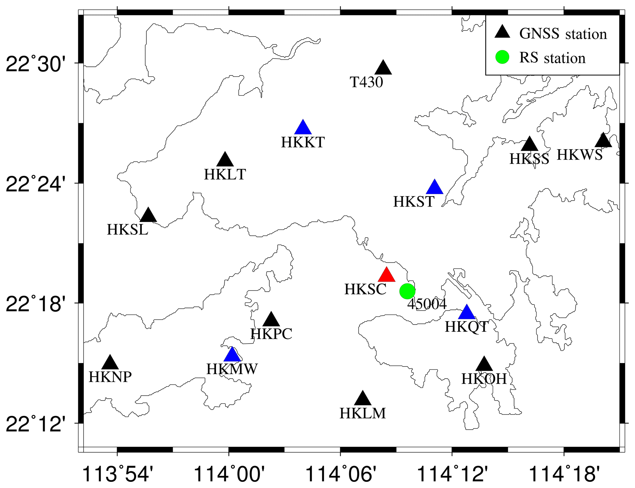
Figure 1 Geographic location of GNSS and radiosonde stations in SatRef of Hong Kong. The blue triangles are used to increase the station density, while the station HKSC marked in red and radiosonde station 45004 marked in green are used to evaluate the performance of tomographic result.

3.2 Determination of horizontal resolution

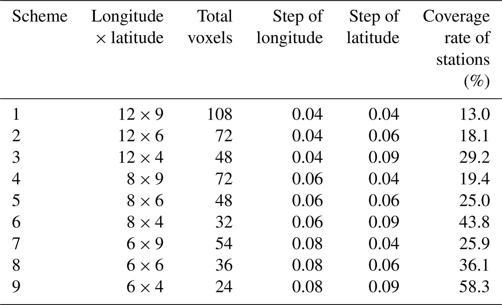
In the procedure of horizontal voxel division, an approach is developed which enables the determination of the optimal horizontal resolution according to the scope of the tomography region as well as the number and distribution of GNSS stations. The specific principle is as follows: by guaranteeing the relatively large coverage rate of GNSS stations located in the bottom layer to optimize the design matrix of the observation equation, and considering a higher horizontal resolution to reflect the atmospheric water vapour distribution in as much detail as possible, a comparative experiment is performed to validate the developed approach of determining horizontal resolution. Here, the coverage rate refers to the ratio between the voxels crossed by satellite rays and total voxels divided in the tomographic area. Nine schemes are designed (Table 1): the number of voxels for the bottom layers and the coverage rate of distributed stations located at the bottom layer are calculated. It can be concluded that Scheme 3 was optimal while considering both the number of voxels divided and the coverage rate of GNSS stations located in the bottom layers.

Table 1 Statistical result of determining a horizontal resolution for nine schemes.

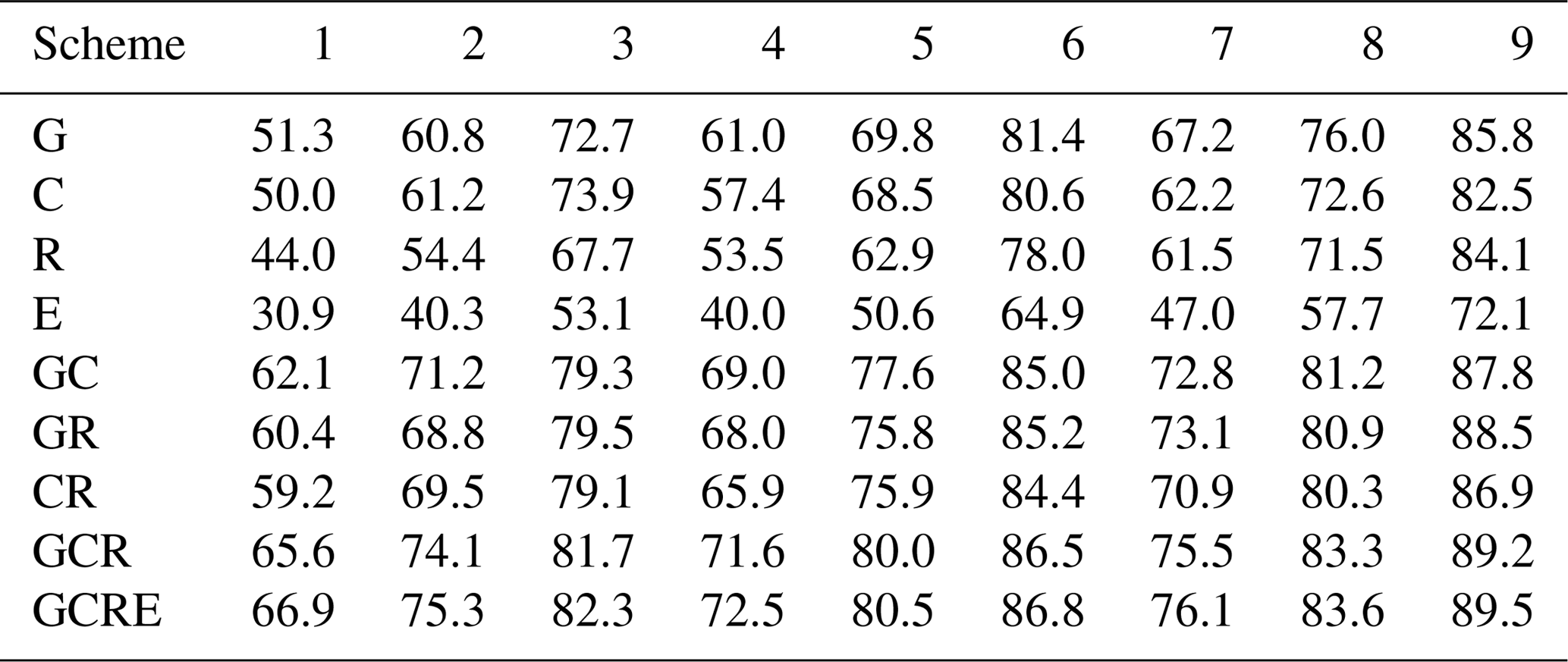
In addition, the coverage rate of the satellite rays for the entire research region is analysed for the date of DOY 4, 2017 under nine combined multi-constellation GNSS observations. In this study, a 5 min time period for each tomography is selected. The specific statistical result is presented in Table 2, where G, C, R, and E refer to GPS, BeiDou, GLONASS, and Galileo, respectively. The conclusion can be drawn that the coverage rate of satellite rays in Schemes 3, 6, 8, and 9 are relatively large. Considering the number of voxels and coverage rate of stations located in the bottom layers, Scheme 3 is also considered as the optimal choice. Further to the conclusion above it can also be concluded that the coverage rate of voxels penetrated by satellite signals for the entire region using two, three, and four-GNSS observations both increased with the minimum coverage rate by approximately 5 % when compared to the single-GNSS conditions.

Table 2 Coverage rate of satellite rays for nine combined multi-constellation GNSS observations (unit: %).

4 Influence of station density on tropospheric tomography

In this section, four schemes are designed to analyse the influence of station density and multi-constellation GNSS data on the reconstructed atmospheric wet refractivity. For Schemes 1 and 2, only 10 GNSS stations are used, as shown by the nine black triangles and one red triangle in Fig. 1, but considering the single-GNSS observation and different multi-constellation GNSS combinations. The single-GNSS observation is abbreviated to G-10, C-10, R-10, and E-10, while the combinations of those are abbreviated to GC-10, GR-10, CR-10, GCR-10, and GCRE-10. For Schemes 3 and 4, all 14 GNSS stations are selected for this tomographic experiment but considering single-GNSS observation and different multi-constellation GNSS combinations. The single-GNSS observation is abbreviated to G-14, C-14, R-14, and E-14, while the combinations of those are abbreviated to GC-14, GR-14, CR-14, GCR-14, and GCRE-14. The following analysis focussed on (1) the investigation of four schemes in the number of GNSS rays used and coverage rate of the voxels penetrated by GNSS rays, and (2) the comparison of reconstructed result with radiosonde data as well as the PPP-estimated SWD values of station HKSC.

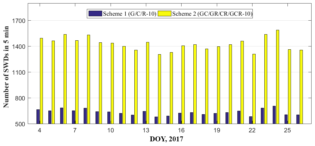
Figure 2 Average number of SWDs used in 5 min for Schemes 1 and 2 during the experimental period.

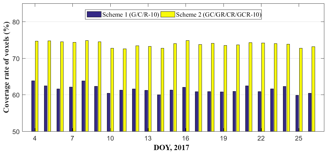
Figure 3 Average coverage rate of voxels penetrated by GNSS signals for Schemes 1 and 2 during the experimental period.

4.1 Comparison of GNSS rays used and the coverage rate of voxels penetrated

The 23 days of data during the period DOY 4–26 2017 are analysed and Table 3 shows the mean value of GNSS rays used and coverage rate of voxels penetrated by signals for the test period. It can be concluded from the statistical results (Table 3) that the number of signals used in Schemes 2 and 4 is apparently large (double to triple) compared to that of Schemes 1 and 3, however, the percentage difference of voxels crossed by rays between Schemes 1/3 and Schemes 2/4 is not as expected except for the cases of E-10 and E-14. The number of Galileo satellite observations is small during the test period; therefore, a low number of signals used and a low coverage rate of voxels penetrated by GNSS signals existed for the cases of E-10 and E-14 in Schemes 1 and 3.

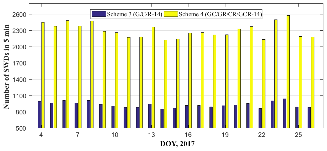
Figure 4 Average number of SWDs used in 5 min for Schemes 3 and 4 during the experimental period.

Figure 5 Average coverage rate of voxels penetrated by GNSS signals for Schemes 3 and 4 during the experimental period.

Table 3 Number of GNSS rays used and the coverage rate of crossed voxels in different schemes during the experimental period.

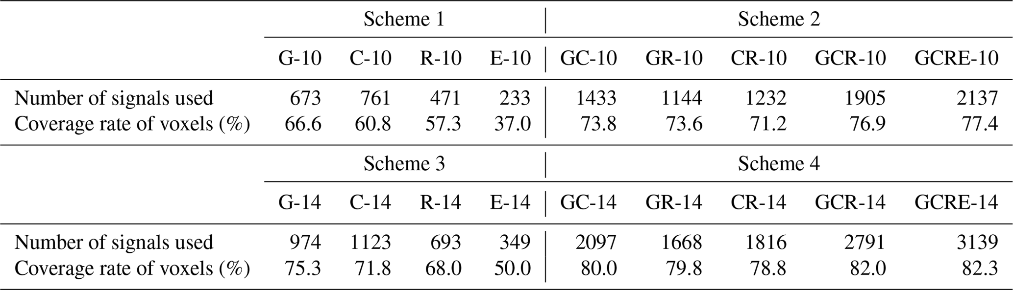
Note: “-14” refers to the statistical result with single-GNSS observations derived from 14 stations. “-10” refers to the statistical result with multi-constellation GNSS observations derived from 10 stations.

To analyse the number of SWDs used and the coverage rate of voxels, the average values of four schemes for each day is calculated in Figs. 2–5. Because the number of Galileo satellites is lower, the cases associated with Galileo are therefore not considered in four schemes. Figures 2 and 4 reveal that the signals used for each day in Schemes 2 and 4 are more than double those in Schemes 1 and 3; however, Figs. 3 and 5 reveal that the proportion of voxels penetrated by GNSS signals in Schemes 2 and 4 are only improved by approximately 12 % and 8.7 %, respectively, than that in Schemes 1 and 3.

From Table 4 we concluded that although the number of satellite rays has been doubled, the percentages of crossed voxels of Schemes 3 and 4 are increased by approximately 12 % and 8 % when compared to the Schemes 1 and 2, respectively. However, the voxels crossed by rays of Schemes 2 and 4 have been improved by 10 % and 6 % when compared to Schemes 1 and 3, respectively, under the conditions that only consider additional four GNSS stations for single-GNSS and multi-GNSS. This indicates that the station density has a more important influence on the coverage rate of voxels crossed by rays than multi-constellation GNSS observations.

Figure 6 RMS error of wet refractivity difference derived from various conditions during the experiment period.

Table 4 Statistical information of GNSS signals used and the percentage of voxels penetrated during the tested period for four schemes.

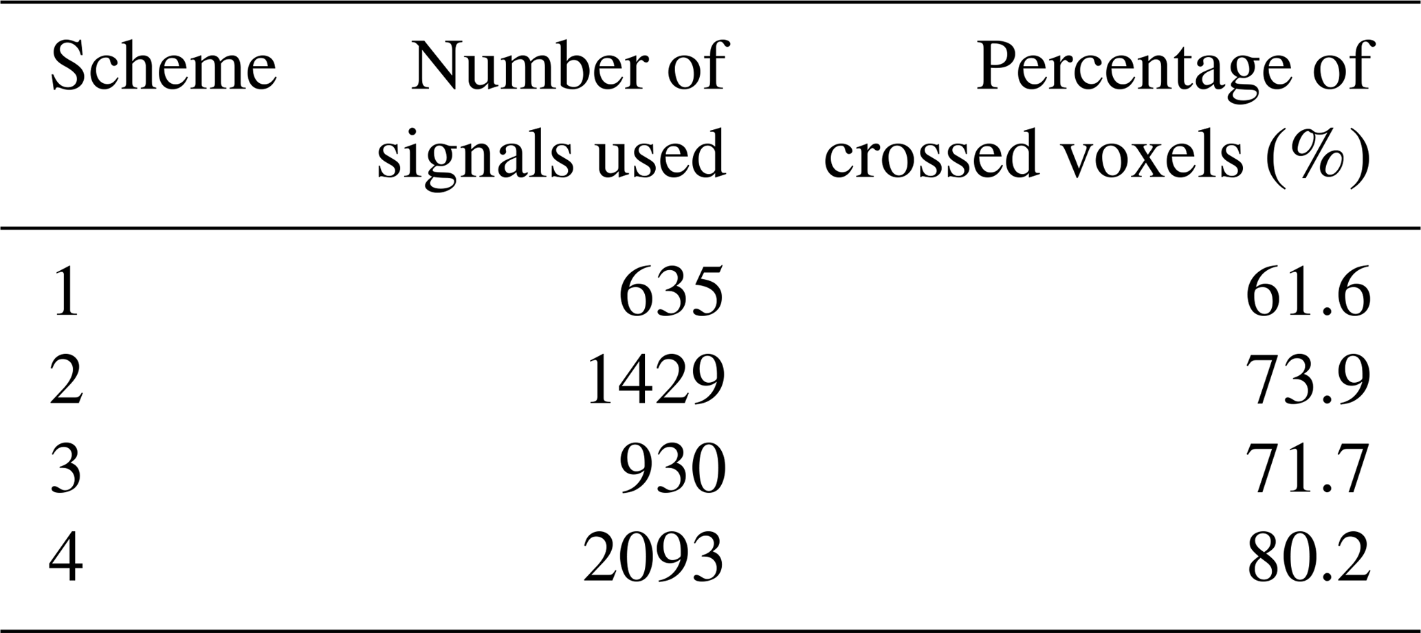
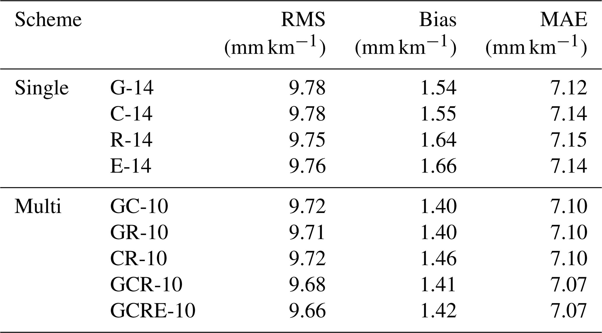
Table 5 Statistical result of RMS, bias, and MAE of wet refractivity difference for different schemes during the experimental period.

4.2 Comparison with radiosonde data

In this section, we further compare the influence of station density on the tomographic result. In the experimental area, there is a radiosonde station, as shown by the green circle in Fig. 1. Several studies have proved that radiosonde data have a high accuracy in providing the water vapour profiles (Niell et al., 2001; Liu et al., 2013), and the result calculated from radiosonde is used as a reference in this paper to evaluate the tomographic result. The comparison experiment of reconstructed wet refractivity profile information using different GNSS observations at the radiosonde station with the radiosonde data is carried out at two specific epochs (00:00 and 12:00 UTC). Figure 6 shows the root mean square (RMS) error of wet refractivity difference between different tomography conditions and radiosonde data. Table 5 gives the specific statistical information pertaining to RMS, bias, and mean absolute error (MAE) for different Schemes. From Fig. 6 and Table 5, we can conclude that the tomographic results using different single- and multi-constellation GNSS observations are similar at the radiosonde location. This is because (1) the a priori information of radiosonde has been imposed into the tomography modelling for the location of radiosonde station and (2) station HKSC is near the radiosonde station, and a relatively large amount of GNSS observations were distributed for the location of radiosonde station. However, such a result cannot represent the quality of reconstructed results of wet refractivity fields for the entire region. Therefore, the accuracy of the tomographic result for the entire research region is further evaluated using the PPP-estimated SWDs below.

Figure 7 Average RMS of SWD residuals for different schemes over the experimental period.

Figure 8 Average RMS of MAE residuals for different schemes over the experimental period.

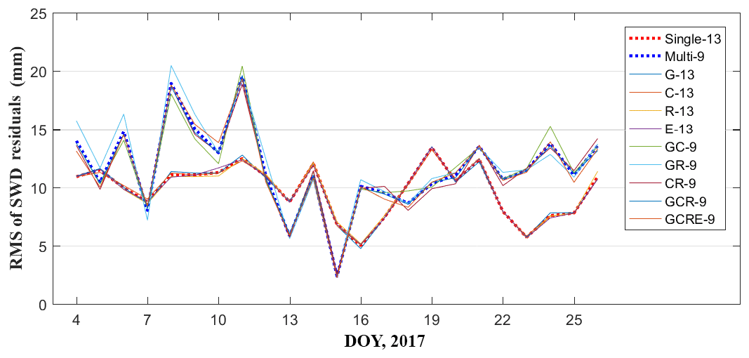
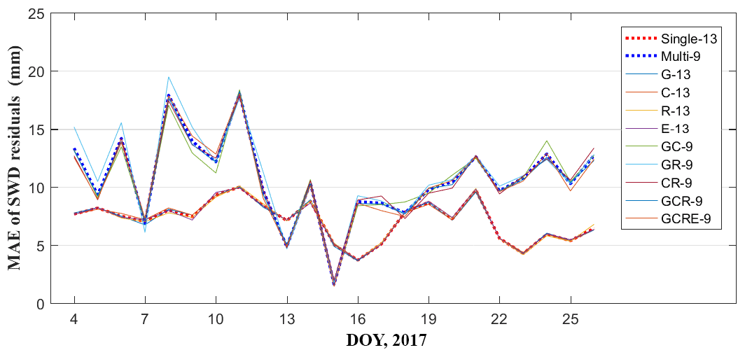
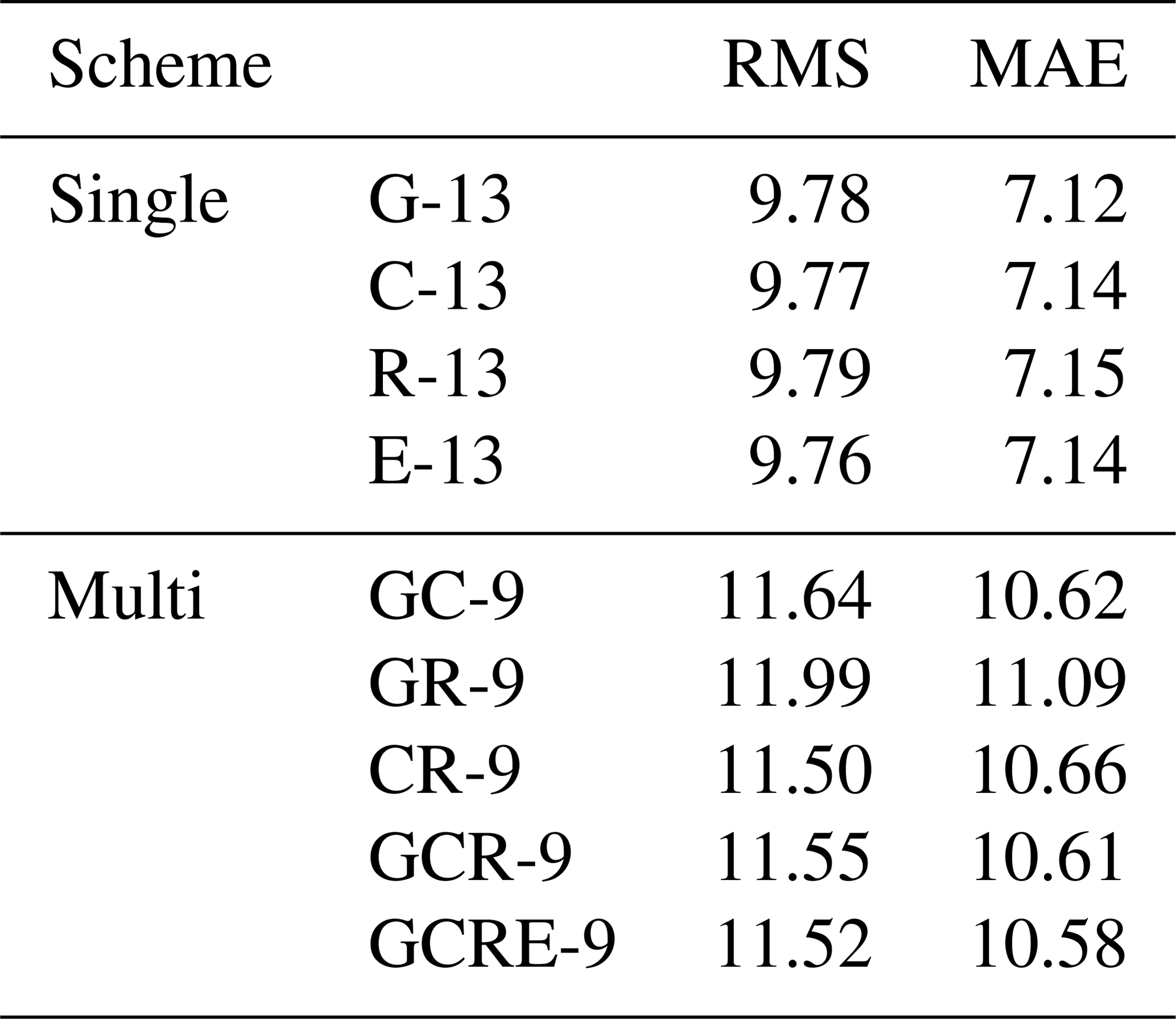
Table 6 Statistical result of RMS and MAE of different tomographic strategies over the experimental period.

4.3 Comparison with PPP-estimated SWDs

To assess the reconstructed result of the entire region, two new schemes are designed: Scheme 1, only the single-GNSS observations of 13 GNSS stations (except for HKSC) are used for reconstructing the atmospheric wet refractivity; Scheme 2, nine GNSS stations, as shown by the black triangles in Fig. 1, are selected using combined multi-constellation GNSS observations. The SWDs of station HKSC are computed based on the different tomographic results and against the GNSS PPP-estimated SWDs. The RMS and MAE of SWD residuals for each day in two schemes are presented in Figs. 7 and 8, where the red dashed line represents the average RMS and MAE obtained under conditions G-13, C-13, R-13, and E-13 while the blue dashed line represents the average RMS and MAE obtained from cases GC-9, GR-9, CR-9, GCR-9, and GCRE-9. Figures 7 and 8 reveal that the average RMS and MAE of Scheme 1 is mostly lower than that of Scheme 2 over the experimental period, which shows that the reconstructed atmospheric wet refractivity field of Scheme 1 over the entire research area is superior to the tomographic result of Scheme 2. Statistical results pertaining to different schemes are listed in Table 6, from which it is seen that, compared to Scheme 2, the average RMS and MAE accuracy of Scheme 1 is increased by 16 % and 33.4 %, respectively. Hence it was concluded that, compared to the tomographic result of multi-constellation GNSS observations, increasing the station density has greater significance for the reconstruction of the atmospheric water vapour field.

5 Analysis of multi-constellation GNSS troposphere tomography

5.1 Comparison of signals used and coverage rate of voxels penetrated

Here, all 14 GNSS stations are selected to reconstruct the atmospheric wet refractivity, and the tomographic results derived from different multi-constellation GNSS observations are compared and analysed. Nine types of single- and multi-constellation GNSS observations are designed in schemes designated G-14, C-14, R-14, E-14, GC-14, GR-14, CR-14, GCR-14, and GCR-14. Before evaluating the performance of the tomographic result, the average number of GNSS signals used and the percentage of voxels penetrated over the experimental period for each tomography step are first analysed (Table 7). Table 7 reveals that compared to schemes G-14 C-14, R-14, and E-14, multi-constellation GNSS schemes have more voxels crossed by rays, but the change is relatively small with respect to the coverage rate of voxels.

Table 7 Statistical information of the number of GNSS rays used and the coverage rate of voxels penetrated.

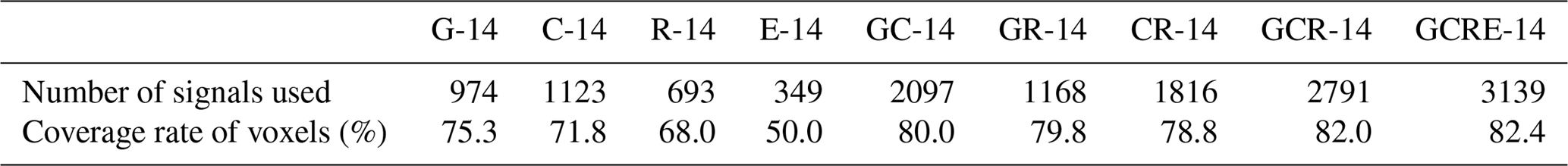
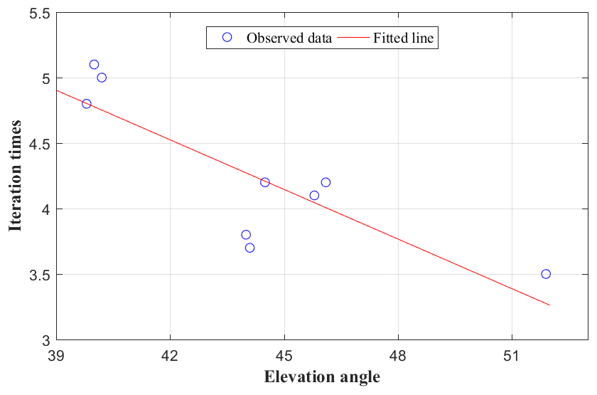
Figure 9 Relationship between iteration times and elevation angle during the experimental period.

5.2 Evaluation of multi-constellation GNSS troposphere tomography

To analyse the performance of the multi-constellation GNSS troposphere tomography, the wet refractivity profile derived from nine schemes is first compared with the result from the radiosonde data thereat. The average RMS, bias, and MAE of wet refractivity difference between different schemes and radiosonde data over the experimental period are calculated (Table 8). As mentioned in Sect. 2, an iterative procedure is required to determine the weighting matrices of different equations in tomographic modelling. Therefore, the number of iterations and the average elevation angle of satellite signals for different schemes are also considered (Table 8). It can be observed from Table 8 that the average RMS, bias, and MAE of different schemes are similar, which reflects the fact that the reconstructed wet refractivity profile obtained from different schemes applied at the radiosonde station have equivalent accuracy.

Table 8 Statistical result of average RMS, bias, MAE, elevation angle, and iteration times for different schemes over the experimental period.

Figure 10 Average RMS of SWD residuals for different schemes over the experimental period.

However, the number of iterations of various schemes are different when determining the weighting matrices of the different types of equations used in tomographic modelling. By analysing the relationship between the number of iterations and elevation angles over the tested period, a negative linear relationship is found between two factors and the fitted data are presented in Fig. 9. Such a negative correlation reveals that the resolving time of tomographic modelling can be decreased with multi-constellation GNSS observations, which is important in the real-time reconstruction of atmospheric water vapour.

Table 9 Statistical result of RMS, bias, and MAE of SWD residuals from different schemes over the experimental period

Figure 11 Average MAE of SWD residuals for different schemes over the experimental period.

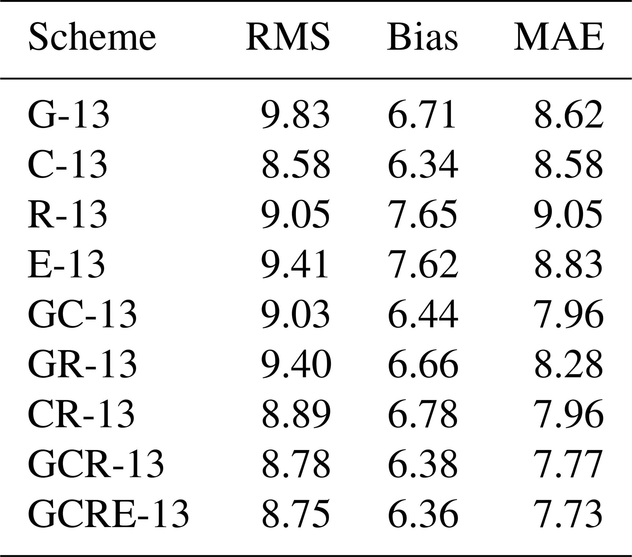
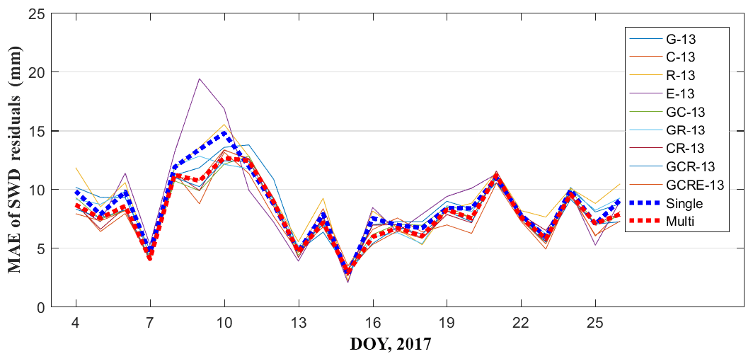
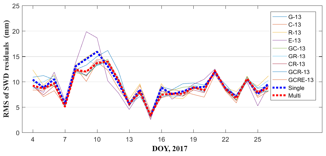
As mentioned above, the accuracy of different schemes evaluated for the location of radiosonde cannot represent the tomographic quality across the entire region; therefore, a further comparison is carried out using only 13 GNSS stations in the network except for station HKSC. The slant wet delays of station HKSC, estimated using multi-GNSS PPP software, are compared with the calculated SWDs derived from different schemes. Figures 10 and 11 show the average RMS and MAE of SWD residuals on each day during the experiment, where the blue dashed line represents the average of RMS and MAE obtained from schemes G-13, C-13, R-13, and E-13, while the red dashed line represents the average of RMS and MAE obtained from schemes GC-13, GR-13, CR-13, GCR-13, and GCRE-13. From those two figures, it was found that the reconstructed quality of atmospheric wet refractivity field data for the entire region using multi-constellation GNSS observations was slightly improved when compared to that using single-constellation GNSS data. By analysing the statistical results pertaining to different schemes (Table 9) it was found that, compared to the single-constellation GNSS troposphere tomography, RMS accuracy of the multi-constellation GNSS troposphere tomography improved by about 10 %.

6 Conclusion

The observed multi-constellation GNSS (GPS, BeiDou, GLONASS, and Galileo) observations have been used to investigate the importance and influence of station density and multi-GNSS constellation data on troposphere tomography. The SWDs of 14 GNSS stations in a network in Hong Kong are estimated using the multi-constellation GNSS PPP software.

For GNSS troposphere tomography, the horizontal resolution of voxels is first determined according to the number of voxels and the coverage rate of GNSS stations located in the bottom layer. A comparative experiment using single- and multi-constellation GNSS data derived from different numbers of stations revealed that increasing the station density improved the quality of tomographic results, with the RMS accuracy of SWD residuals increasing by about 16 % when compared to the result of using multi-constellation GNSS troposphere tomography. In addition, compared to the single-constellation GNSS observations, troposphere tomography using multi-constellation GNSS data can (1) reduce the resolving time when determining the weighting matrices of different equations used in tomographic modelling, which has practical significance for the real-time reconstruction of atmospheric water vapour profiles, and (2) improve the quality of tomographic results to a certain extent.

The upcoming full operability of the multi-constellation GNSS is expected to increase the number of SWDs used for troposphere tomography. Although the improvement of reconstructed results is not as expected, it was mainly determined by the spatial distribution of GNSS stations, multi-constellation GNSS troposphere tomography is also worth studying, especially for potential application of this technique in real-time atmospheric water vapour reconstruction.