Monitoring potential ionospheric changes caused by the Van earthquake (M_w7.2)

Many scientists from different disciplines have studied earthquakes for many years. As a result of these studies, it has been proposed that some changes take place in the ionosphere layer before, during or after earthquakes, and that the ionosphere should be monitored in earthquake prediction studies. This study investigates the changes in the ionosphere created by the earthquake with a magnitude of M_w=7.2 in the northwest of Lake Erçek, which is located to the north of the province of Van in Turkey on 23 October 2011 and at 13:41 local time (−3 UT) with the epicenter of 38.75^∘ N, 43.36^∘ E using the TEC values obtained by the global ionosphere models (GIMs) created by IONOLAB-TEC and CODE. In order to see whether the ionospheric changes obtained by the study in question were caused by the earthquake or not, the ionospheric conditions were studied by utilizing indices providing information on solar and geomagnetic activities (F10.7 cm, Kp, Dst).

One of the results of the statistical test of the TEC values obtained from both models is positive and negative anomalies obtained for the times before, on the day of and after the earthquake, and the reasons for these anomalies are discussed in detail in the last section of the study. As the ionospheric conditions on the analyzed days were highly variable, it was thought that the anomalies were caused by geomagnetic effects, solar activity and the earthquake.

1 Introduction

The ionosphere is the part of the atmosphere at the altitudes of 60 to 1100 km where there are ions and free electrons in considerable amounts that can reflect electromagnetic waves. It completely covers the thermosphere, one of the main layers of the atmosphere, but also includes some of the mesosphere and the exosphere.

Total electron content (TEC), which is defined as free electrons along a cylinder with a cross section of 1 m², is a suitable parameter to monitor the changes in the ionosphere. All signals that contain data that pass through or get reflected from the ionosphere, which is highly irregular and difficult to model, are affected by the structure of this layer.

Calculation of TEC is used directly to investigate the structure of the ionosphere. TEC is represented by the unit of TECU, and 1 TECU equals 10¹⁶ el m⁻² (Schaer, 1999). TEC is expressed in two ways: STEC (slant total electron content), the free electron content calculated along the slanted line between the receiver and the satellite; and VTEC (vertical total electron content), the free electron content calculated along the zenith of the receiver (Langley, 2002).

Figure 1 OZAL, IZMI, AFYN, KAYS and BING stations analyzed in the present work.

The ionosphere reacts to geomagnetic effect, solar activity, diurnal and seasonal effects, and earthquake, and these factors cause irregularities in the ionosphere (Namgaladze et al., 2012; Li and Parrot, 2018).

Ionospheric changes have been studied in more than 20 countries today as precursors of earthquakes. Definition of ionospheric anomalies and feasibility studies of seismo-ionospheric precursors is still ongoing (Liu et al., 2010; He et al., 2012; Kamogawa and Kakinami, 2013; Heki and Enomoto, 2015; Pulinets and Davidenko, 2014; Masci et al., 2015; Yildirim et al., 2016; He and Heki, 2017; Kelley et al., 2017; Rozhnoi et al., 2015; Thomas et al., 2017; Ulukavak and Yalcinkaya, 2017).

Our study aim is to investigate ionospheric changes possibly caused by the Van earthquake while taking into account solar activity and magnetic storm effect. The Van earthquake has a very complex structure in terms of ionospheric conditions. When the levels of solar activity (F10.7 cm) and magnetic storm (Kp and DsT) are considered, ionospheric conditions appear to be highly active before and after the earthquake. Therefore results obtained by statistical test should be interpreted carefully.

2 Methodology

2.1 IONOLAB-TEC method

The IONOLAB-TEC method developed by the Department of Electrical and Electronics Engineering of Hacettepe University is a JAVA application that uses the Regularized TEC (D-TEI) algorithm (Arikan et al., 2004).

In this application, they developed a method that estimates VTEC values by using all GPS signals measured at a period of time in a day. While the measurements taken from the satellites with elevations of 60^∘ or higher are used, the measurements from the satellites with elevations of 10 to 60^∘ are weighted by a Gauss function. The data from satellites with elevations lower than 10^∘ are not included in calculations to reduce multipath effects. In this method raw GPS data were used to determine VTEC value.

Table 1 OZAL Station global ionosphere model anomaly table.

Table 2 OZAL Station IONOLAB-TEC anomaly table.

2.2 Global ionosphere model (GIM)

Global ionospheric maps are published in the IONEX (IONosphere map EXchange) format in a way that covers the entire world. The institutions that produce these maps in the world include CODE (Center for Orbit Determination in Europe, Switzerland), DLR (Fernerkundungstation Neustrelitz, Germany), ESOC (European Space Operations Centre, Germany), JPL (Jet Propulsion Laboratory, California), NOAA (National Oceanic and Atmospheric Administration, United States), NRCan (National Resources, Canada), ROB (Royal Observatory of Belgium, Belgium), UNB (University of New Brunswick, Canada), UPC (Polytechnic University of Catalonia, Spain), and WUT (Warsaw University of Technology, Poland). In this study we used the GIM-TEC values produced by CODE in the IONEX format. On the dates they were analyzed, the temporal resolution of the TEC values was 2 h, while their positional resolution was 2.5^∘ by latitude and 5^∘ by longitude. In order to calculate TEC values for a point whose latitude and longitude are known on the GIM-TEC maps created by CODE using more than 300 GNSS receivers around the world, the four TEC values that cover the point and the two-variable interpolation formula are given below.

$$\begin{array}{ll}{\displaystyle }& {\displaystyle }{E}_{\mathrm{int}}\left({\mathit{\lambda }}_{\mathrm{0}}+p\mathrm{\Delta }\mathit{\lambda },{\mathit{\beta }}_{\mathrm{0}}+q\mathrm{\Delta }\mathit{\beta }\right)=\left(\mathrm{1}-p\right)\left(\mathrm{1}-q\right)E_{\mathrm{0.0}}\\ \text{(1)}& {\displaystyle }& {\displaystyle }+p\left(\mathrm{1}-q\right)E_{\mathrm{1.0}}+q\left(\mathrm{1}-p\right)E_{\mathrm{0.1}}+pq{E}_{\mathrm{1.1}}\end{array}$$

p and q: 0≤p, q<1 (Schaer, 1999); Δλ and Δβ: longitude and latitude difference grid widths; λ₀ and β₀: initial longitude and latitude values; E_0.0, E_1.0, and E_0.1 and E_1.1: TEC values known in neighboring points; E_int: TEC value to be found.

3 Analysis to determine earthquake-related TEC changes

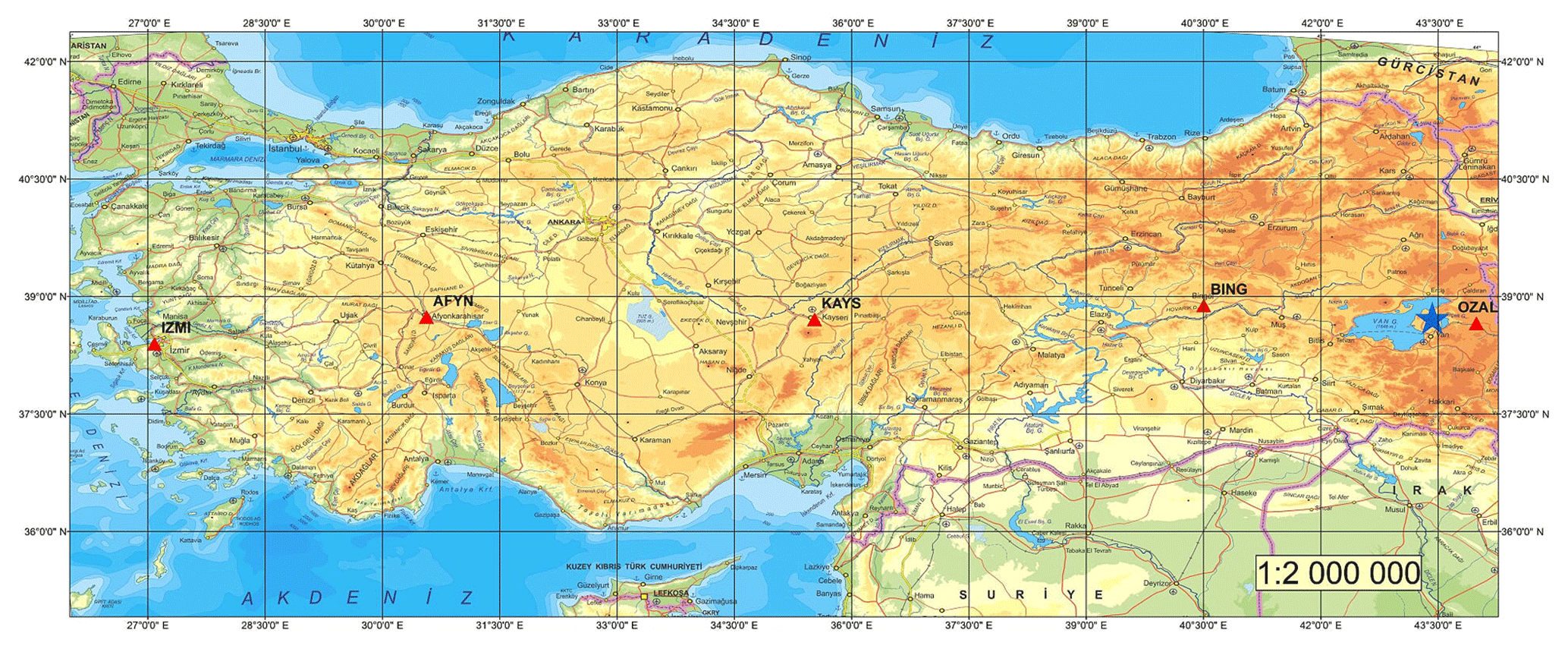
In order to investigate earthquake-related TEC changes, the TEC values for OZAL Station (TUSAGA-Active CORS-TR) close to the epicenter's GPS station was analyzed to determine the TEC value using the IONOLAB-TEC and GIM-TEC models. The correlation coefficient was obtained for the TEC values from both models between the dates 13 October and 2 November 2011 for the stations above. In addition to that, spatial analysis was applied to determine distribution characteristics of the ionospheric changes.

Figure 1 shows the stations analyzed (represented by red triangles) and the epicenter of the earthquake (represented by a blue star). TEC values with the temporal resolution of 2 h obtained from both the IONOLAB-TEC and GIM-TEC models for OZAL (37.06^∘ N, 36.15^∘ E) (station which is nearest to the epicenter of the earthquake), and the correlation coefficient was computed to explain the linear relationship between the two models. On the other hand, TEC values were also obtained using a GIM to explain spatial changes in the ionosphere for IZMI (38.23^∘ N, 27.04^∘ E), AFYN (38.44^∘ N, 30.33^∘ E), KAYS (38.42^∘ N, 35.31^∘ E) and BING (38.53^∘ N, 40.30^∘ E) stations.

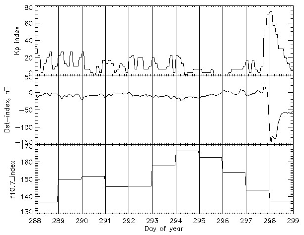
Figure 2 (Kp⋅10), DsT, and F10.7 cm index variation from 288 to 299 in 2011 (https://omniweb.gsfc.nasa.gov/form/dx1.html, last access: 5 July 2018).

Table 3 IZMI Station GIM-TEC anomaly table.

Table 4 AFYN Station GIM-TEC anomaly table.

In order to determine the outlier values among the TEC values with a 2 h temporal resolution from both models, the TEC values obtained from both models between the dates 1 and 10 October 2011, which were considered quiet in terms of geomagnetic and solar activity, were used to determine the upper boundary (UB) and the lower boundary (LB). By utilizing the TEC values from both models, the UB and LB values were calculated using the formulae x+3σ and x−3σ. Here, x is the mean TEC value for the relevant epoch and σ is the standard deviation. If the TEC value in any epoch is higher than the upper boundary, it is a positive anomaly. Similarly, if it is lower than the lower boundary, it is a negative anomaly. In order to investigate whether the anomalies before, on the day of and after the earthquake were caused by the earthquake or not, we also examined the (Kp⋅10), Dst and F10.7 cm indices, which provided information on the geomagnetic and solar activity for the days in which anomalies were detected.

Table 5 KAYS Station GIM-TEC anomaly table.

Table 6 BING Station GIM-TEC anomaly table.

Table 7 Total amount of anomaly in TECU for analyzed days.

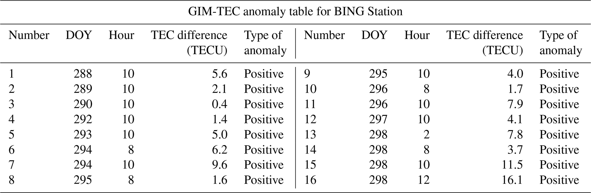
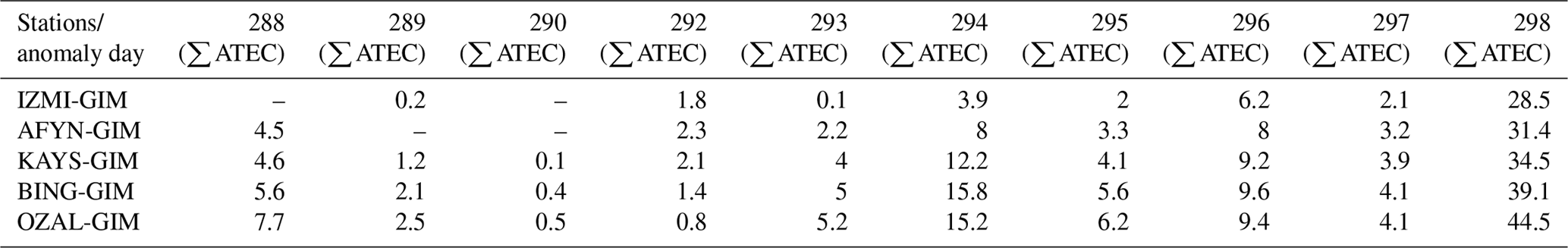
Figure 2 shows the (Kp⋅10), Dst and F10.7 cm indices that provide information on geomagnetic and solar activity from 15 to 25 October 2011.

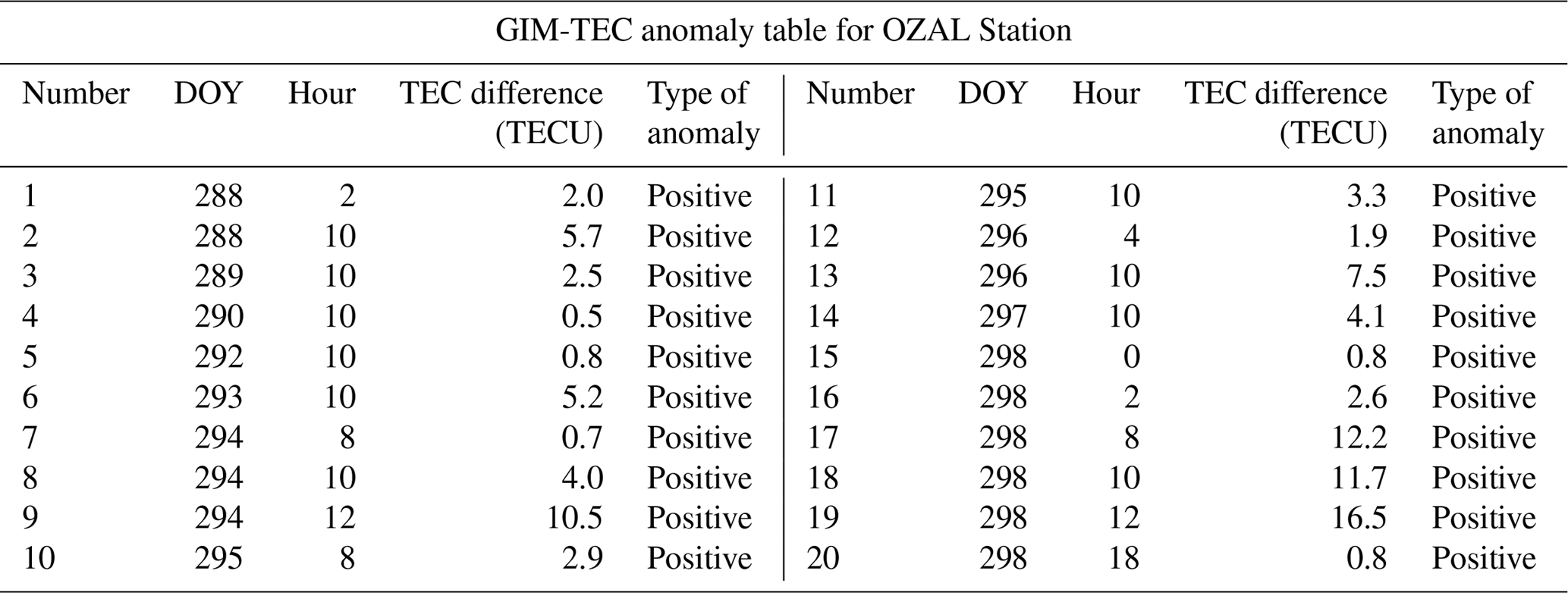
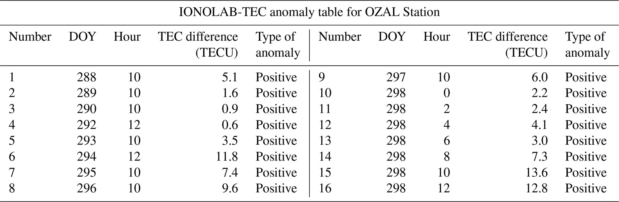
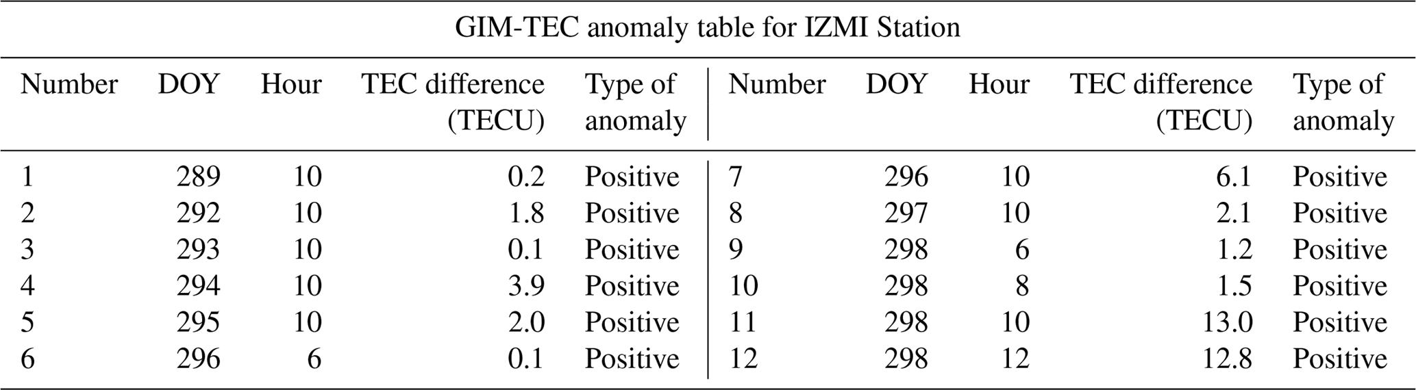
The correlation coefficient r between the TEC values calculated by both methods for OZAL Station was 0.98, demonstrating a strong positive relationship. The anomaly tables for this station are provided below (Tables 1 and 2).

In order to determine whether anomalies were caused by the earthquake or not, we also monitored spatial changes in TEC. In this regard, we investigated the IZMI, AFYN, KAYS, and BING stations' TEC changes using GIMs. These receivers are located at the same latitude as OZAL Station, and thus we can obtain spatial TEC changes in Turkey for analyzed days.

Tables 1–6 also depict the day and hour in which anomalies were observed, and the amount and type of the anomaly. The numbers of anomalies obtained in both models were very close to each other. The F10.7 cm index values between days 288 and 292 were 136.9, 150, 151.6, 145.7, and 146.1 sfu. Nwanko and Chakrabarti (2013) state that while F10.7 cm > 151 sfu is strong solar activity, 100 sfu < F10.7 cm < 150 sfu indicates moderate solar activity. The index values show that there was usually moderate solar activity. Therefore, the anomalies in question may be related to the earthquake or solar activity. The index values for days 293, 294, 295 and 296 (the day of the earthquake) were 157.8, 166.3, 162.5 and 153.9 sfu, respectively. These values indicate strong solar activity. On the other hand, the ionosphere layer was quiet on these days in terms of geomagnetic conditions. The numbers of anomalies were higher than during days 288–292 due to solar activity being stronger during these last days. Since solar activity was moderate on day 297, the number of anomalies dropped. The solar activity on day 298 was moderate, but there was strong geomagnetic activity (Dst −147 nt, $\mathrm{Kp}\cdot \mathrm{10}=\mathrm{73}$). The reason for the high numbers of anomalies on day 298 in both models is believed to be geomagnetic activity. This magnetic storm has caused different amounts of TEC variation for all stations.

As another indicator, we extract ∑ATEC (total TEC difference) to determine the total amount of anomaly day by day for each analyzed day. ∑ATEC shows the total amount of anomaly for an analyzed day. For example, 4.5 TECU is the sum of the total TEC difference for the 24 h of 288 in 2011 for AFYN Station.

Table 7 shows total anomaly summary results obtained from analysis results. Positive anomalies were observed before and after the earthquake and amounts of anomalies are nearly equal to each other in this earthquake. In addition to that, ∑ATEC differences between stations are also similar to each other for each analyzed day. Therefore this similarity causes spatial variation of the ionosphere.

Considering the analyzed days in general for all stations, it may be seen that it is difficult to identify earthquake-related anomalies as the solar activity and geomagnetic conditions before and after the earthquake were not quiet. Therefore, it is believed that the anomalies detected in the stations on days 293–296 may be related to the earthquake and/or solar activity, and the anomalies on days 297 and 298 may be related to the earthquake, solar activity and/or geomagnetic activity.

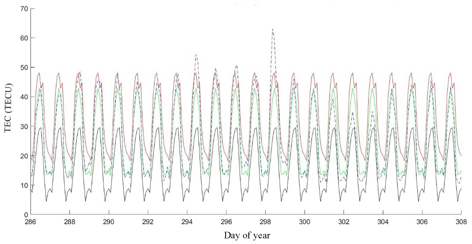
Figure 3 GIM-TEC values for OZAL Station. The black line shows lower bound TEC values, the red line demonstrates upper bound TEC values, the green line shows mean TEC values and the dotted line indicates observed TEC values for every epoch.

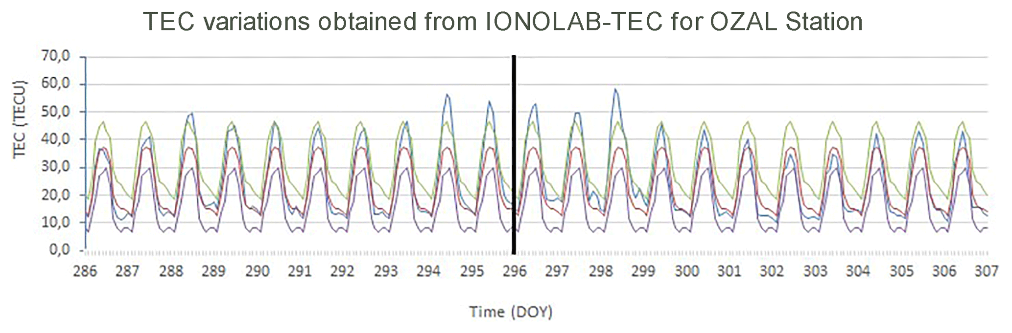
Figure 4 IONOLAB-TEC values for OZAL Station. The purple line shows lower bound TEC values, the bottle green line demonstrates upper bound TEC values, the red line shows mean TEC values and the blue line indicates observed TEC values for every epoch.

Figure 5 GIM-TEC values for IZMI Station. The black line shows lower bound TEC values, the red line demonstrates upper bound TEC values, the green line shows mean TEC values and the dotted line indicates observed TEC values for every epoch.

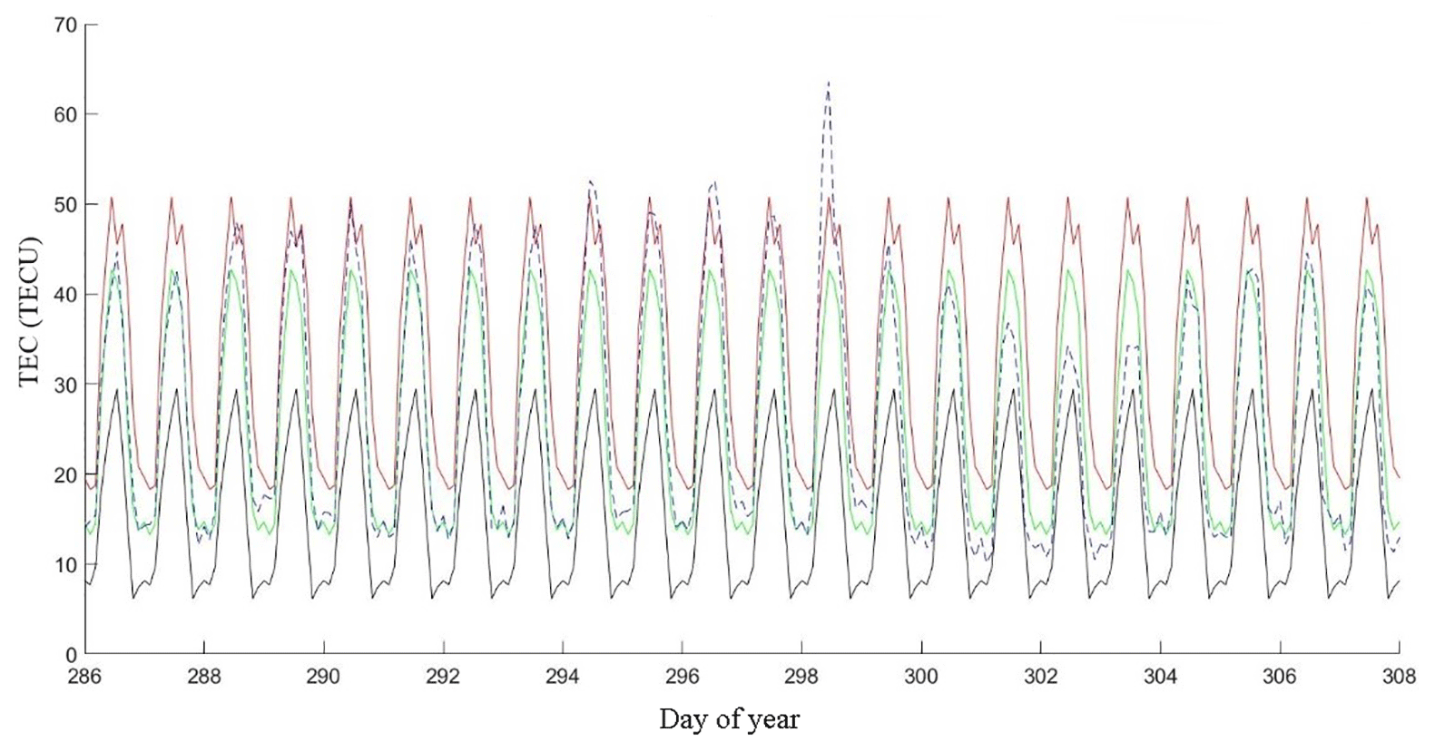
Figure 6 GIM-TEC values for AFYN Station. The black line shows lower bound TEC values, the red line demonstrates upper bound TEC values, the green line shows mean TEC values and the dotted line indicates observed TEC values for every epoch.

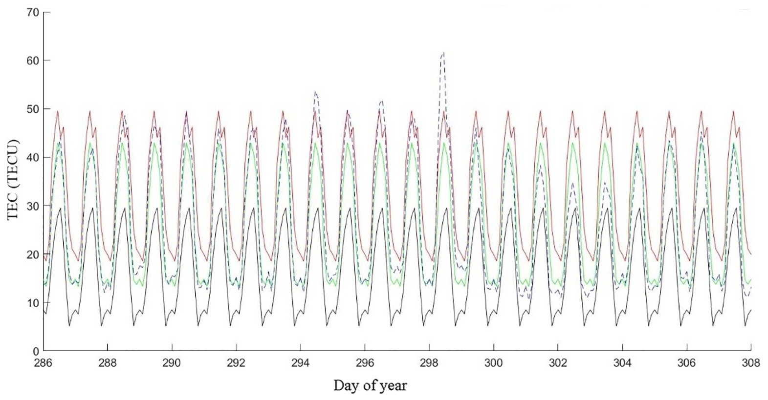
Figure 7 GIM-TEC values for KAYS Station. The black line shows lower bound TEC values, the red line demonstrates upper bound TEC values, the green line shows mean TEC values and the dotted line indicates observed TEC values for every epoch.

4 Discussion and conclusion

Seismic ionospheric evaluations of the Van earthquake have also been studied by many researchers (Arikan et al., 2004; Namgaladze et al., 2012; Rolland, 2013; Şentürk et al., 2018). Arikan et al. (2004) and Namgaladze et al. (2012) determined some anomalies before and after the earthquake, but solar and magnetic conditions were not taken into account. On the other hand Şentürk et al. (2018) also obtained abnormal days before and after the earthquake and they evaluated solar activity and magnetic storm conditions for these abnormal days to explain possible causes of anomalies in detail. Some previous studies have also investigated both space-weather and earthquake effects in the ionosphere (Yao et al., 2012; Le et al., 2013). They especially state that TEC enhancement may be related to geomagnetic storm and earthquake.

The Şentürk et al. (2018) study also shows that there is no obvious anomaly caused only by earthquake. Therefore they suggest that a multidisciplinary study would be useful to identify ionospheric changes as an earthquake precursor under the disturbed space-weather conditions. This approach shows that their results agree with our study. Apart from our method, the He et al. (2012) study states that detection of the earthquake anomaly can be removed from measurement using the multiresolution wavelet transform (MWT) method, removing other effects like solar radiation. However, this technique's main problem is that F10.7 cm is one value, and TEC is 2 h temporal resolution for 1 day. Thus we think that different temporal resolutions of F10.7 cm and TEC cause big obstacles to distinguishing the F10.7 effect on TEC values directly.

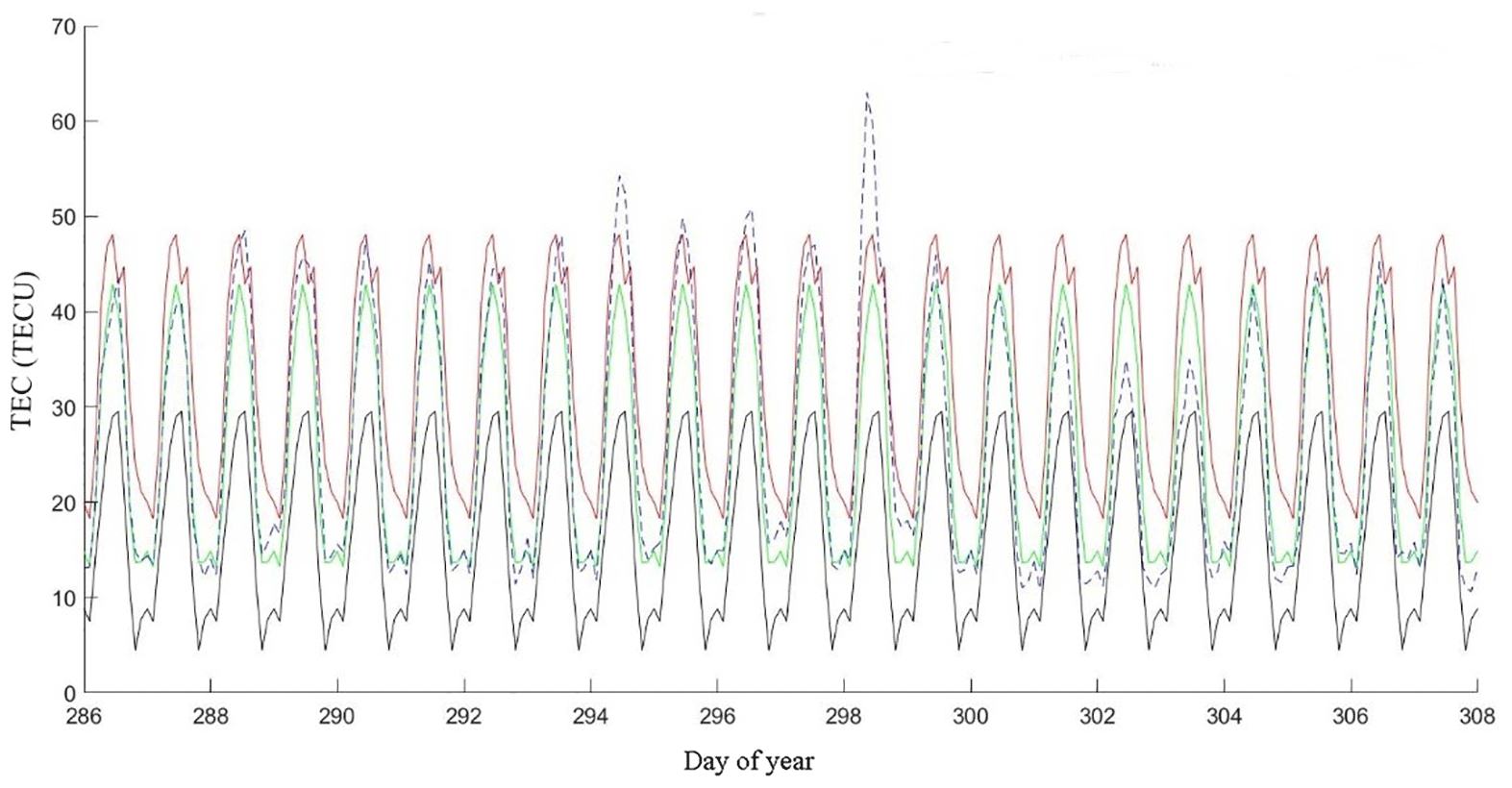
Figure 8 GIM-TEC values for BING Station. The black line shows lower bound TEC values, the red line demonstrates upper bound TEC values, the green line shows mean TEC values and the dotted line indicates observed TEC values for every epoch.

In the scope of this study, the TEC values for stations IZMI, AFYN, KAYS, and BING were obtained using the GIM-TEC and TEC values also obtained using the GIM-TEC and IONOLAB-TEC methods for OZAL Station. In the comparison of the obtained values, it was seen that there was a high correlation between the TEC values obtained by the two models for OZAL Station. In order to detect earthquake-related TEC changes better, the TEC values created from both models for the period of 13 October–2 November 2011 were used as a reference to determine the upper bound and lower bound values. As a result of the statistical test, anomalies were found in all analyzed stations for before, on the day of and after the earthquake. In order to understand whether the anomalies obtained in both models were earthquake-related, the ionospheric conditions, geomagnetic activity and solar activity on the analyzed days were examined using the Kp, Dst and F10.7 cm indices.

Consequently, it was determined that the positive anomalies observed on days 286–292 may be related to moderate solar activity and/or the earthquake, and the positive anomalies observed on days 293, 294, 295, and 296 (day of the earthquake) may be related to strong solar activity and/or the earthquake. Moderate solar activity and strong geomagnetic activity were observed for day 298, so the numbers of anomalies in both models increased dramatically. This increase is considered to be related to geomagnetic activity. The anomaly on day 298 may be related to the earthquake, geomagnetic effects and/or solar activity. The finding that the ionospheric conditions were variable on the analyzed days makes it highly difficult to identify earthquake-related ionospheric changes. Therefore, interdisciplinary study is needed to determine the earthquake-related part of the change in question.