the Creative Commons Attribution 4.0 License.
the Creative Commons Attribution 4.0 License.
 | 06 Mar 2019
Spring and summer time ozone and solar ultraviolet radiation variations over Cape Point, South Africa
Jelena V. Ajtić
Hassan Bencherif
Nelson Bègue
Jean-Maurice Cadet
Caradee Y. Wright
The correlation between solar ultraviolet radiation (UV) and atmospheric ozone is well understood. Decreased stratospheric ozone levels which led to increased solar UV radiation levels at the surface have been recorded. These increased levels of solar UV radiation have potential negative impacts on public health. This study was done to determine whether the break-up of the Antarctic ozone hole has an impact on stratospheric columnar ozone (SCO) and resulting ambient solar UV-B radiation levels at Cape Point, South Africa, over 2007–2016. We investigated the correlations between UV index, calculated from ground-based solar UV-B radiation measurements and satellite-retrieved column ozone data. The strongest anti-correlation on clear-sky days was found at solar zenith angle 25∘ with exponential fit R2 values of 0.45 and 0.53 for total ozone column and SCO, respectively. An average radiation amplification factor of 0.59 across all SZAs was calculated for clear-sky days. The MIMOSA-CHIM model showed that the polar vortex had a limited effect on ozone levels. Tropical air masses more frequently affect the study site, and this requires further investigation.
- Article
(4249 KB) - Full-text XML
- BibTeX
- EndNote


Solar ultraviolet (UV) radiation is a part of the electromagnetic spectrum of energy emitted by the Sun (Diffey, 2002). Solar UV radiation comprises a wavelength band of 100–400 nm; however, not all wavelengths reach the Earth. Solar UV radiation is divided into UV-A, UV-B and UV-C bands depending on the wavelength. The UV-C and UV-A bands cover the shortest and longest wavelengths, respectively. The UV-B part of the spectrum spans a wavelength range between 280 and 315 nm (WHO, 2017). The reason behind this sub-division of UV radiation is a large variation in biological effects related to the different wavelengths (Diffey, 2002). Moreover, an interaction of different UV bands with the atmospheric constituents results in an altered UV radiation reaching the surface: all UV-C and ∼90 % of UV-B radiation is absorbed, while the UV-A band is mostly unaffected (WHO, 2017). The amount of solar UV-B radiation at the surface of the Earth is largely impacted by the amount of atmospheric ozone (Lucas and Ponsonby, 2002), but also several other factors, such as altitude, solar zenith angle (SZA), latitude and pollution (WHO, 2017). The SZA has a significant impact on the amount of surface solar UV-B radiation (McKenzie et al., 1996). Under clear-sky conditions and low pollution levels, atmospheric ozone (of which approximately 90 % is found in the stratosphere) absorbs solar UV-B radiation (Fahey and Hegglin, 2011). A study in the south of Brazil found a strong anti-correlation between ozone and solar UV-B radiation on clear-sky days using fixed SZAs (Guarnieri et al., 2004).
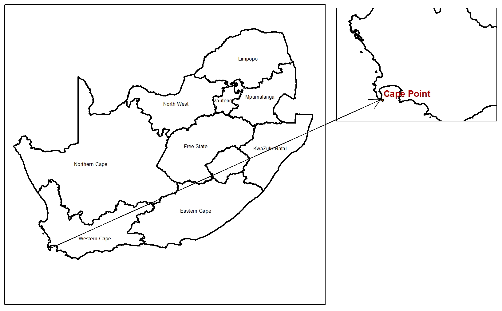
Figure 1The map of South Africa and the location of the SAWS Cape Point Weather station in the Western Cape.
Anthropogenic and natural factors can cause changes in the amount of atmospheric ozone. Unlike natural ozone variability which is mostly of a seasonal nature and therefore has a reversible character, human activities, such as the release of ozone-depleting substances, have led to a long-term ozone decline in a greater part of the atmosphere (Bais et al., 2015), and, in turn, to higher levels of solar UV-B radiation at the Earth's surface (Fahey and Hegglin, 2011). An outstanding example of ozone depletion is the formation of the Antarctic ozone hole, a phenomenon discovered in the 1980s (Farman et al., 1985). Each austral spring, a severe ozone depletion occurs under the unique conditions in the Antarctic polar vortex, decreasing total ozone column (TOC) below 220 Dobson units (DU), a threshold defining the ozone hole.
The Antarctic ozone hole has been extensively studied (WMO, 2011). Apart from its direct influence on the ozone amounts in the Southern Hemisphere (Ajtić et al., 2004; de Laat et al., 2010) the Antarctic ozone hole affects a wide range of atmospheric phenomena as well as the climate of the Southern Hemisphere. For example, ozone depletion over Antarctica has altered atmospheric circulation, temperature and precipitation patterns in the Southern Hemisphere during the austral spring and summer (Brönnimann et al., 2017; Bandoro et al., 2014). Another notable consequence of decreased atmospheric ozone is an increase in solar UV radiation at the surface of the Earth, which has been supported by experimental evidence (Herman and McKenzie, 1998). This anti-correlation and association with the Antarctic ozone hole has been confirmed at Lauder, New Zealand (McKenzie et al., 1999).
Our analysis investigated the anti-correlation between the content of ozone in the atmosphere and solar UV-B radiation over the Western Cape Province, South Africa. The objectives in our study were (1) to determine the climatology of solar UV-B radiation and the climatology of TOC and stratospheric column ozone (SCO) for Cape Point, South Africa; (2) to determine clear-sky days for Cape Point and use them to analyse the anti-correlation between solar UV-B radiation and TOC, on the one hand, and solar UV-B radiation and SCO, on the other hand; (3) to identify low TOC and SCO events at Cape Point during spring and summer months; (4) to use a transport model to determine the origin of ozone-poor air observed during the identified low-ozone events; and (5) to explore whether the Antarctic ozone hole influenced the identified low-ozone events at Cape Point. To the best of our knowledge these objectives, in a South African context, and in relation to increased solar UV-B radiation over South Africa directly related to the Antarctic ozone depletion, have not been studied before.
2.1 UV data
The study site was Cape Point (34.35∘ S, 18.50∘ E, 230 m a.s.l.), a weather station in the Western Cape, South Africa (Fig. 1). The station is one of the World Meteorological Organization (WMO) Global Atmosphere Watch (GAW) baseline monitoring sites. It is located around 60 km south of Cape Town and although it is considered free of air pollution (Slemr et al., 2008), it may still be affected by maritime aerosols. Since aerosols can have a pronounced effect on the amount of UV radiation reaching the surface (Bais et al., 2015), our choice of Cape Point offers a setting in which a modification of the UV-B radiation by anthropogenic aerosols can be overlooked.
Solar UV-B radiation data, with the original hourly recording interval, were obtained from the South Africa Weather Service (SAWS) for Cape Point station for the period 2007–2016. The solar UV-B radiation measurements were made with the Solar Light Model Biometer 501 Radiometer. The biometer measures solar UV radiation with a wavelength of 280–320 nm. The measured solar UV radiation is proportional to the analogue voltage output from the biometer with a controlled internal temperature (Solarlight, 2014). Two different instruments were used at Cape Point between 2007 and 2016: Instrument 3719 (January 2007–March 2016) and Instrument 1103 (April–December 2016). Both instruments were calibrated at Solar Light in June 2006 according to the “Calibration of the UV radiometer – Procedure and error analysis”. During the period of operation three inter-comparisons were conducted using recently calibrated standard reference instruments. The inter-comparisons aimed to verify that the instruments in operation were recording accurate measurements and the inter-comparisons did not include homogenisation of the data or the application of different calibration factors.
Measurements are given in minimal erythemal dose (MED) units where 1 MED is defined by SAWS as 210 Jm−2 and any incorrect or missing values were indicated in the dataset. During October 2016, the measured MED values exceeded the expected values and were corrected with a correction factor as recommended by the SAWS. Despite periods of missing data during the study years, there were 3129 days of useable solar UV-B data for Cape Point. To convert from instrument-weighted UV radiation to erythemally weighted UV radiation, a correction factor was applied as the instrument does not measure the full spectral range of the UV index (Seckmeyer et al., 2005; Cadet et al., 2017). Solar UV-B radiation values in MED were converted to UV index (UVI) using
Since the correlation between solar UV-B radiation and ozone can be better observed when controlling SZA (Booth and Madronich, 1994), we also calculated SZA. First, we computed 10 min SZAs using an online tool, the Measurement and Instrument Data Centre's Solar Position Calculator (MIDC SPA) (https://midcdmz.nrel.gov/solpos/spa.html, last access: February 2017), which utilises the date, time and location of the site of interest and has an accuracy of ±0.0003∘ (Reda and Andreas, 2008). Second, from the 10 min SZAs we calculated hourly averages.
2.2 Column ozone data
TOC and SCO data were obtained for 2007–2016 (inclusive) for the grid area which was bound by the following coordinates – west: 16.5∘ E, south: 36.35∘ S, east: 20.6∘ E, north: 31.98∘ S. This grid area limited the TOC and SCO data to the area directly above Cape Point. The daily TOC data were measured with the Ozone Monitoring Instrument – Total Ozone Mapping Spectrometer (OMI – TOMS) on NASA's Aura satellite. OMI has a spatial resolution of 0.25∘, which results in a ground resolution at nadir with a range of 13 km × 24 km to 13 km × 48 km (Levelt et al., 2006). Relative to other ozone observations, OMI has a bias of 1.5 % (McPeters et al., 2015). In the Southern Hemisphere, OMI-TOMS data have a lower seasonal dependence compared to the Northern Hemisphere. Overall, observations are within 3 % of Dobson and Brewer spectrophotometer observations (Balis et al., 2007).
The daily SCO data were measured with the Microwave Limb Sounder (MLS) instrument on NASA's Aura satellite. The MLS ozone data consisted of ozone profiles at 55 pressure levels and SCO values up to the thermal tropopause. The thermal tropopause is determined by the temperature data taken by the MLS instrument. The ozone profiles were used between 261 and 0.02 hPa (Livesey et al., 2017). The daily SCO values were extracted from the MLS data files. SCO observations from the MLS overestimate ozone in the stratosphere over 30∘ S but this overestimation is lower than compared to the Northern Hemisphere (Jiang et al., 2007). MLS SCO observations have a high correlation coefficient, 0.96–0.99, with OMI SCO observations (Huang et al., 2017).
2.3 Transport model
The Mesoscale Isentropic Transport Model of Stratospheric Ozone by Advection and Chemistry (Modèle Isentropique du transport Méso-échelle de l'ozone stratosphérique par advection avec CHIMIE or MIMOSA-CHIM) was used to identify the source of ozone-poor air above Cape Point. MIMOSA-CHIM results from the off-line coupling of the MIMOSA dynamical model (Hauchecorne et al., 2002) from the Reactive Processes Ruling the Ozone Budget in the Stratosphere (REPROBUS) chemistry model (Lefèvre et al., 1994). The ability of MIMOSA-CHIM to simulate and analyse the transport of stratospheric air masses has been highlighted in several previous studies over the polar regions (Kuttippurath et al., 2013, 2015; Tripathi et al., 2007; Semane et al., 2006; Marchand et al., 2003). The dynamical component of the model is forced by meteorological data such as wind, temperature and pressure fields from the European Centre for Medium-Range Weather Forecasts (EMCWF) daily analyses. The dynamical component of potential vorticity (PV) was used to trace the origin of ozone-poor air masses. PV can be used as a quasi-passive tracer when diabatic and frictional terms are small. Therefore, over short periods of time, PV is conserved on isentropic surfaces following the motion (Holton and Hakim, 2013). A spatial area from 10∘ N to 90∘ S was used for the model with a resolution. The model has stratospheric isentropic levels ranging from 350 to 950 K. The MIMOSA-CHIM model created an output file for every 6 h. Simulations for each low-ozone event were initialised to run for at least 14 days prior to the low-ozone event to account for the model spin-up period. The PV maps were analysed at isentropic levels that correspond to 18, 20 and 24 km above ground level, thus covering the lower part of the ozone layer (Sivakumar and Ogunniyi, 2017).
2.4 Method
The climatologies of UVI, TOC and SCO were determined using the available days with data. These would provide a reliable baseline to which observations from specific days could be compared. Next, clear-sky days were determined from the solar UV-B radiation data based on a method that looks at the diurnal pattern of UV-B radiation. Once the clear-sky days had been determined, the correlation analysis between ozone and UVI was calculated using two methods. Only using clear-sky days removed the effect of clouds on UV-B radiation. Lastly, we determined low-ozone events and used the MIMOSA-CHIM model to identify the origin of ozone-poor air masses.
2.4.1 Climatologies
The hourly UVI value was averaged for each day in a specific month across the 10-year period and was used to determine the UVI climatology at Cape Point. All days were used to determine the climatology. The TOC and SCO climatologies were calculated using monthly averages.
2.4.2 Determination of clear-sky days
Cloud cover has a range of impacts on surface UV radiation, and therefore calculating cloud-free conditions is important to understand cloud impacts on UV radiation. Partly cloudy skies can reduce or increase UV radiation depending on the position of the Sun and clouds, while overcast skies decrease radiation (Bodeker and McKenzie, 1996; Bais et al., 2015). Due to the different spectral properties of clouds, the ability to detect clouds through solar radiation measurements is dependent on the wavelength of the spectrum that is measured (Zempila et al., 2017). Several studies (Bodeker and McKenzie, 1996; Zempila et al., 2017) have attended to determine cloud-free conditions and have all shown the challenges, in particular, for thin cloud conditions. Thus, determining cloud-free days is a step towards removing a contribution of all factors except amount of atmospheric ozone. As shown by McKenzie et al. (1991) a stronger correlation between ozone and solar UV-B radiation may be obtained if the days with clouds are removed.
The SAWS Cape Point site has no cloud cover data available. For that reason, we used a clear-sky determination method by Bodeker and McKenzie (1996) to find cloudy days and consequently remove them from our further analysis. First, days with solar UV-B measurements, TOC and SCO data were divided into seasons: summer – December, January, February (DJF), autumn – March, April, May (MAM), winter – June, July, August (JJA), and spring – September, October, November (SON). Then, clear-sky days were determined using three different tests.
The first test only considered the daily linear correlation between the UVI values measured before solar noon and the values after solar noon. Solar noon was determined as the hour interval with the lowest SZA value. Days with a linear correlation below 0.8 in the DJF, MAM and SON seasons were removed and were considered to be cloudy days. The first test was not performed on the winter season, when the UVI values, as well as the correlation values, were low.
The second test looked for a monotonic increase before solar noon and a monotonic decrease after solar noon for each day. On clear-sky days, UVI values before and after solar noon should monotonically increase and decrease, respectively. If monotonicity did not hold for the UVI values on a specific day, it was assumed that there was some cloud present on that day. The monotonicity test was performed for all seasons. It is interesting to note that at Cape Point, the second test of the clear-sky determination method identified more clear-sky afternoons than clear-sky mornings.
The third test removed days when the UVI values did not reach a threshold maximum value. This test was applied to all seasons. The threshold was determined as a value of 1.5 standard deviations (1.5 SD) below the UVI monthly average. The monthly average and standard deviations were determined from the solar UV-B radiation climatology for Cape Point.
Prior to applying the clear-sky determination method to the Cape Point UV-B radiation data, we tested the methodology against measurements from the Cape Town weather station where cloud cover data are available. In the test, we used the daily 06:00 and 12:00 UTC cloud cover observations, and randomly selected two years for the validation. The results showed that when the observations indicated more than four-eighths of cloud present, our methodology also identified these days as cloudy. Furthermore, we examined the diurnal radiometric curves from another year and found that the determined clear-sky days' radiometric curves closely followed the expected diurnal radiometric curve. This validation implied that the clear-sky tests removed approximately 87 % of cloudy days. Overall, approximately 500 days were determined to be clear-sky days that had UV-B, TOC and SCO data and they were used in our further analyses. For the DJF, MAM, JJA and SON seasons there were 150, 104, 137 and 102 clear-sky days respectively.
2.4.3 Correlations
In addition to removing anthropogenic aerosols by choosing an air-pollution-free site and alleviating cloud effects by looking only at the clear-sky days, the correlation between solar UV-B radiation and ozone can be better observed when controlling SZA (Booth and Madronich, 1994). The correlation calculations were performed at fixed SZAs. The strength of the correlation between the amount of ozone (TOC and SCO data) and UVI was determined using the first-order exponential fit (Guarnieri et al., 2004):
where y= UVI and x= ozone values (TOC or SCO).
The significance of the goodness of fit was determined for a 95 % confidence interval. The log-UVI (y axis) values were taken to test whether the goodness-of-fit R2 values of the exponential fits were statistically significant (Hazarika, 2013).
2.4.4 Radiation amplification factor
The radiation amplification factor (RAF) describes a relationship between ozone values and solar UV-B radiation (Booth and Madronich, 1994). The RAF was introduced as a quantification of the effect that decreased ozone concentrations have on solar UV-B radiation levels. The RAF is a unitless coefficient of sensitivity and here we used its definition given by Booth and Madronich (1994) in Eq. (3). The RAF value at fixed SZAs was calculated using a specific clear-sky day compared to another random clear-sky day from a different year (Booth and Madronich, 1994).
where O3 and are the first and second ozone values and UVI and UVI′ are the first and second UV measurements, respectively.
2.4.5 Low-ozone days
Days of low TOC and SCO values were determined from the set of clear-sky days, but only during spring and summer seasons, when solar UV radiation levels are highest. Days of low TOC values might not have had low SCO values and vice versa. Low TOC and SCO days were determined as days when the respective values were below 1.5 SD from the mean as determined in the climatology analyses (Schuch et al., 2015).
We then used the MIMOSA-CHIM model to identify whether the origin of ozone-poor air masses was from the polar region. In other words, on low-ozone days we looked into the maps of advected PV from MIMOSA-CHIM to identify the source of ozone-poor air parcels over the study area.
3.1 Climatologies and trends
3.1.1 UVI climatology
The monthly means of UVI for Cape Point during 2007–2016 were calculated as a function of time of the day and month of the year (Fig. 2). This climatology provides a reliable baseline against which observations can be compared and reveals the general patterns of the UVI signal recorded at the surface over the investigated 10-year period.

Figure 2The UVI climatology for all sky conditions at Cape Point. The x axis starts with the month of July and ends with June.
At Cape Point, the UVI maximum value of approximately 8 UVI occurs between 13:00 and 15:00 South African Standard Time (SAST), which corresponds to between 11:00 and 13:00 UTC (Fig. 2). The maximum UVI values are not centred on the local noon, implying that more UV radiation reaches this site in the afternoon. Indeed, as previously mentioned, our clear-sky determination method identified more clear-sky afternoons than clear-sky mornings (Sect. 2.4.2), which, under the assumption that cloud cover at Cape Point generally attenuates UV radiation reaching the surface, could explain the observed shift in the UVI maximum to about 14:00 SAST.
The seasons of maximum (DJF) and minimum (JJA) solar UV-B radiation at Cape Point are as expected for a site in the Southern Hemisphere and are similar to those found in studies at other South African sites, namely Pretoria, Durban, De Aar, and Port Elizabeth and Cape Town (Wright et al., 2011; Cadet et al., 2017). The maximum UVI values found in this study occur at similar times to Cadet et al. (2017) and Wright et al. (2011).
3.1.2 Ozone climatologies
At Cape Point, TOC (with the maximum of 303.4 DU) and SCO (with the maximum of 273.1 DU) values peaked during September and decreased to a minimum in February for SCO (232.65 DU) and April for TOC (254.49 DU) (Fig. 3). The variations in TOC and SCO are largest at the maximum values and smallest at the minimum values. Over Irene in Pretoria the greatest variation in SCO was seen during spring (Paul et al., 1998), which is in agreement with our results. It is suggested that this variability in TOC is due to the movement of mid-latitude weather systems which move further north during the Southern Hemisphere winter (Diab et al., 1992). The climatology of TOC over South Africa is mainly affected by atmospheric dynamics rather than by the effects of atmospheric chemistry (Bodeker and Scourfield, 1998).
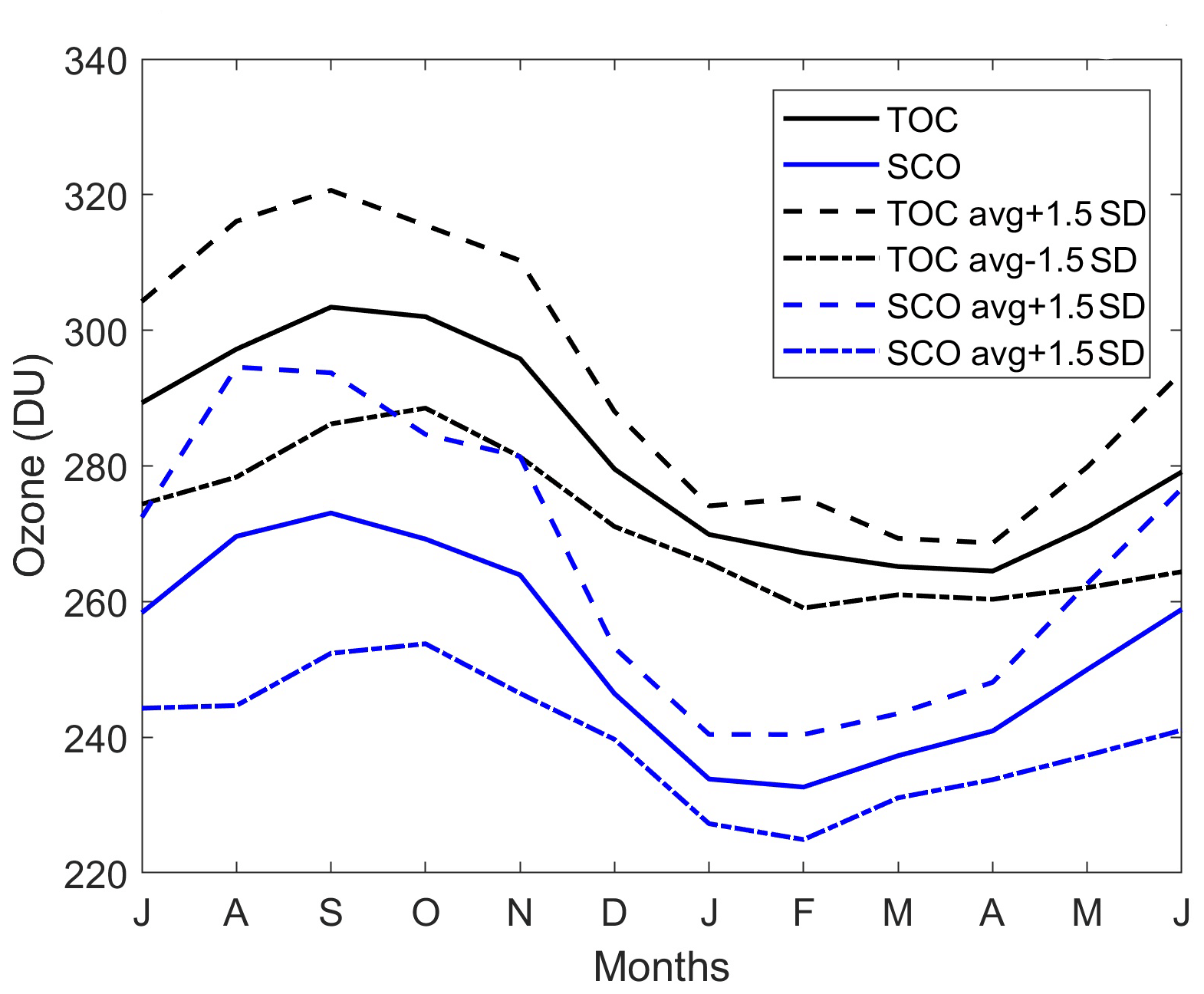
Figure 3Monthly means ±1.5 SD for total ozone column and stratospheric column ozone starting in July and ending in June.
The increase in TOC values during the winter months and the maximum during spring months are due to an ozone-rich mid-latitude ridge that forms on the equator side of the polar vortex. The ridge is a result of a distorted meridional flow caused by the Antarctic polar vortex that forms in late autumn. The vortex prevents poleward transport of the air and thus allows for a build-up of ozone-rich air in mid-latitudes. The lower TOC values over summer could be due to the dilution effect of ozone-poor air from the Antarctic ozone hole. The dilution effect occurs when the vortex breaks up (Bodeker and Scourfield, 1998; Ajtić et al., 2004).
3.2 Correlation between the amount of ozone and UVI
The first-order exponential goodness-of-fit R2 values at fixed SZAs (Table 1) describe the anti-correlation between the amount of ozone in the atmosphere and UVI. The strongest anti-correlation was found at a fixed SZA 25∘ for both TOC and SCO. In this study the first-order exponential fit was used to describe the anti-correlation between ozone and solar UV radiation as in some instances this is best described with a non-linear fit (Guarnieri et al., 2004). A study on the anti-correlation between solar UV-B irradiance and TOC in southern Brazil found that the percentage of the R2 values for exponential fits (66.0 %–85.0 %) explained the variations in solar UV-B irradiance due to TOC variations on clear-sky days at the same fixed SZA categories used in our study (Guarnieri et al., 2004).
Table 1The correlation statistics for amount of ozone and UVI at Cape Point on clear-sky days.
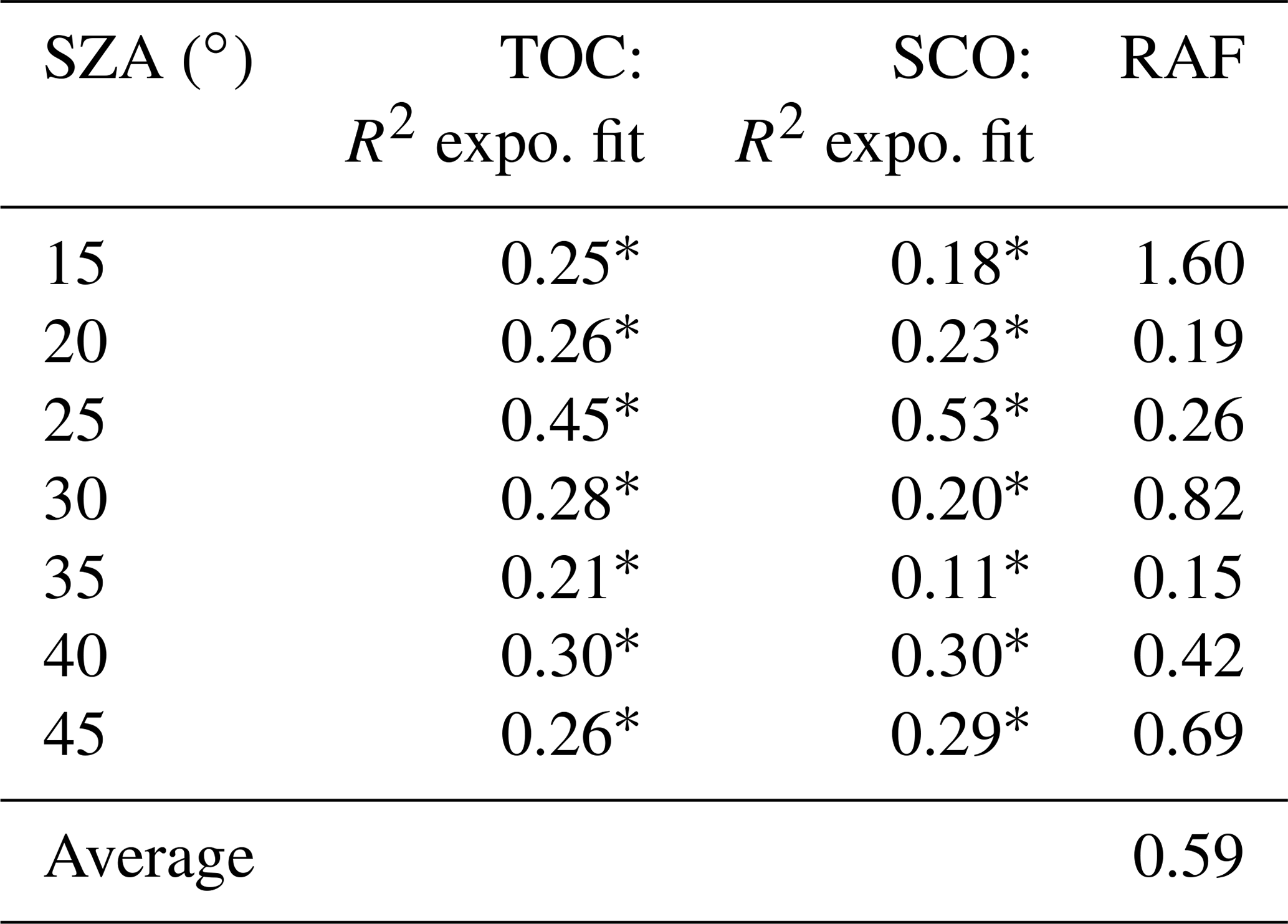
* Indicates R2 values were statistically significant at a 95 % confidence interval.
The exponential R2 values of TOC found at Cape Point at a fixed SZA were much lower than those for southern Brazil (Guarnieri, et al., 2004). In our study and in other studies the R2 value is smaller at the largest SZAs (Guarnieri et al., 2004; Wolfram et al., 2012). The correlation at smaller SZAs may be weaker than expected due to the limited number of data points at smaller SZAs. An improvement can be made on the correlations between SZA by discriminating between morning and afternoon SZAs.
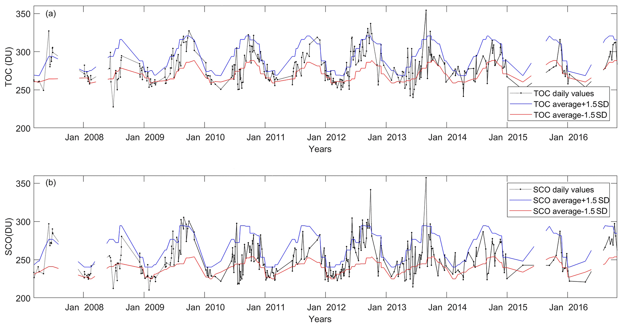
Figure 4TOC (a) and SCO (b) values on clear-sky days over Cape Point and an indication of the average ±1.5 SD limits. Each dot corresponds to a TOC and SCO measurement on a clear-sky day from 2007 to 2016. Interrupted lines indicate missing data.
At Cape Point, the RAF value for clear-sky days range between 0.15 and 1.60 with an average RAF value of 0.59. This can be interpreted as follows: for every 1 % decrease in TOC, UV-B radiation at the surface will increase by 0.59 %. RAF values specific to ozone and solar UV studies found in the literature range between 0.79 and 1.7 (Massen, 2013). RAF values have been used to describe the effect of other meteorological factors such as clouds and aerosols on surface UV radiation (Serrano et al., 2008; Massen, 2013). The differences to the RAF values found here and those found in the literature can be attributed to changes in time and location (Massen, 2013).
Salt build-up on the biometer at Cape Point may also have contributed to the accuracy of measurements taken by the biometer. Solar UV-B radiation data with a higher temporal resolution (e.g. 10 min) may have provided more data points for the analysis at fixed SZAs. Higher temporal resolution solar UV-B radiation data would have improved the determination of clear-sky days. An improvement on the correlation and RAF values could be made by investigating the aerosol concentrations over the station.
3.3 Low-ozone events
Low-ozone events which occurred during the SON and DJF months were identified from the time series of TOC and SCO data on clear-sky days (Fig. 4). The highest frequency of low TOC and low SCO events occurred during January months and January and December months, respectively.
The low TOC and low SCO events along with the respective percentage decrease in TOC and SCO (Table 2) represent some of the largest decreases that occurred in DJF and SON seasons between 2007 and 2016 on clear-sky days. The DJF seasons of 2009–2010 and 2015–2016 are classified as El Niño years (Climate Prediction Center Internet Team, 2015). During these seasons higher TOC levels are expected over the mid-latitude regions (Kalicharran et al., 1993). From the identified low TOC events at Cape Point, none occurred during El Niño years.
This analysis aimed to discuss effects of stratospheric ozone and tropospheric ozone on surface UV-B radiation variations. When TOC and SCO reductions are similar, the effect of stratospheric ozone decrease is dominant. Conversely, when the reduction of TOC is high, and the reduction of SCO is low, the effect of tropospheric ozone is dominant.
Table 2Identified low-ozone events on clear-sky days at Cape Point during spring and summer months and the percentage decrease calculated from the relative climatological monthly mean.
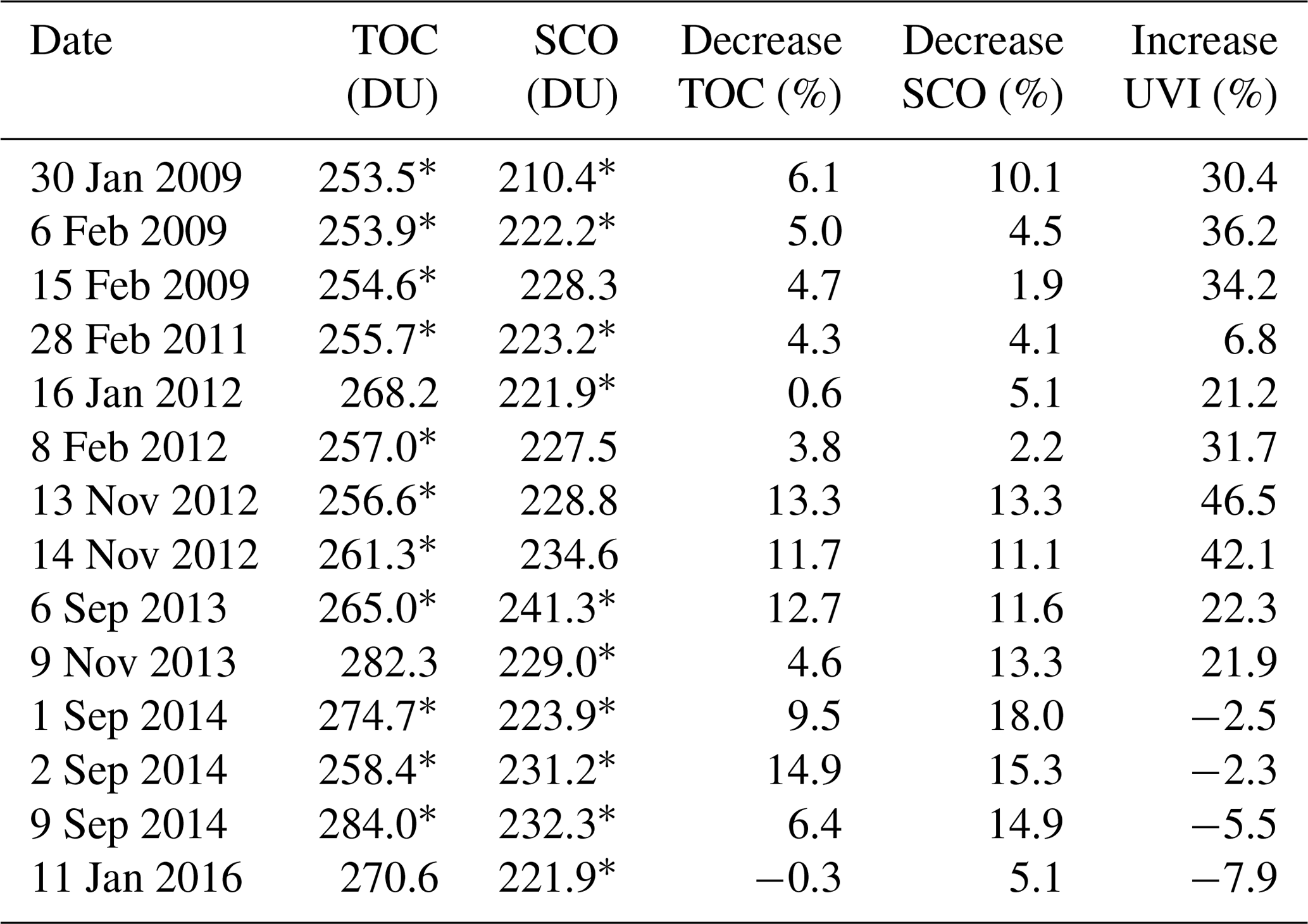
* Indicates whether the low-ozone event was due to low TOC and/or low SCO values.
All of the low-ozone events which occurred during January were due to decreased SCO. A decrease of 10.1 % in SCO was recorded on 30 January 2009 with a TOC decrease of 6.1 %. During February months we obtained the weakest reductions in TOC and SCO. Low-ozone events that occurred during September were mainly due to stratospheric ozone decreases, with the largest ozone reduction recorded on 1 September 2014 (18 % in SCO reduction) (Table 2).
We compared the UVI levels recorded during low-ozone events within the SON and DJF seasons to the UVI climatology to determine if the ozone reductions reflected on the UVI levels during low-ozone events. At Cape Point, the largest increases in the UVI levels were recorded for low-ozone events during November. The largest increase (46.5 %) in UVI occurred on 13 November 2012.
In the Southern Hemisphere, during the spring season (SON) low-ozone events are predominately due to the distortion and filamentation of the Antarctic ozone hole and to the dilution of the associated polar vortex. The dilution effect occurs later in the early summer season, when ozone-poor air masses from the polar region mix with air masses from the mid-latitudes and result in decreased ozone concentrations (Ajtić et al., 2004). There are no studies that refer to low-ozone events at Cape Point. In South Africa, a decrease in TOC was observed over Irene (25.9∘ S, 28.2∘ E) during May 2002 when TOC levels were 8 %–12 % below normal and at a minimum of 219.0 DU (Semane et al., 2006). The relative position of the surface high or low pressure can result in increases or decreases in TOC. The effect on TOC by weather systems is seasonally dependent (Barsby and Diab, 1995).
The increased levels of solar UV-B radiation found in this study due to low SCO events are similar to those found at other Southern Hemisphere sites (Gies et al., 2013; McKenzie et al., 1999; Abarca et al., 2002). It is possible that low-ozone events that occurred over Cape Point during 2007–2016 have not been included. These events might have fallen outside the methods used in this study or were not considered due to the availability of solar UV-B radiation, TOC or SCO data. Moreover, it should be noted that the Cape Point site being located at 34∘ S, at the southern limit of the tropical stratospheric reservoir. Cape Point can be affected by dynamical and transport processes, and therefore air masses of different latitude origins can pass over it. Indeed, over our study period from September to February, the obtained low-ozone event could be of polar origin (i.e. in relation with the extension and distortion of the polar vortex) or of tropical origin (i.e. in relation with isentropic air masses transport across the subtropical barrier, as reported by Semane et al., 2006, and Bencherif et al., 2011, 2007). The following sub-section discusses low-ozone events with regard to the dynamical situations and origins of air masses above the study site.
3.4 Origin of ozone-poor air
In this section the model results from MIMOSA-CHIM are shown for a selection on low-ozone events. The latitude origin of air masses was classified according to the colour scale on the PV maps. Blue colours indicate air masses with relatively high PV values, implying their polar origins, while red colours indicate relatively low PV values of tropical origin.
The origin of the air masses for low-ozone events in January (Table 3) and February (Table 4) shows a consistent pattern: in the lower parts of the stratosphere, at 425 K, the air was of tropical origin; higher up, at 475 K, it was of mid-latitude origin; and at 600 K, air masses from the polar region were above Cape Point. This pattern is illustrated in the PV maps from MIMOSA-CHIM of the low-ozone event on 16 January 2012 (Fig. 5), which best demonstrates all January events. During this event, we identified low SCO (Table 2). Similarly, the PV maps from MIMOSA-CHIM for the low-ozone event on 6 February 2009 (Fig. 6) best demonstrate the situation for February months.
Our results imply that the low-ozone events during the months of January and February were not directly influenced by the Antarctic ozone hole as by that time, the polar vortex had already broken up. However, it is possible that these events are a consequence of the ensuing mixing of the polar ozone-poor air that reduces the mid-latitude ozone concentrations (Ajtić et al., 2004).
Table 3Origin of ozone-poor air at isentropic levels for low-ozone events in January.
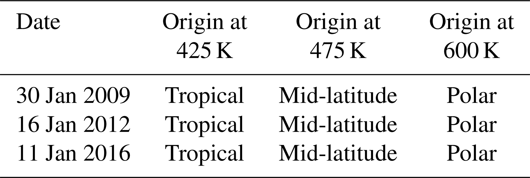
Table 4Origin of ozone-poor air at isentropic levels for low-ozone events in February.
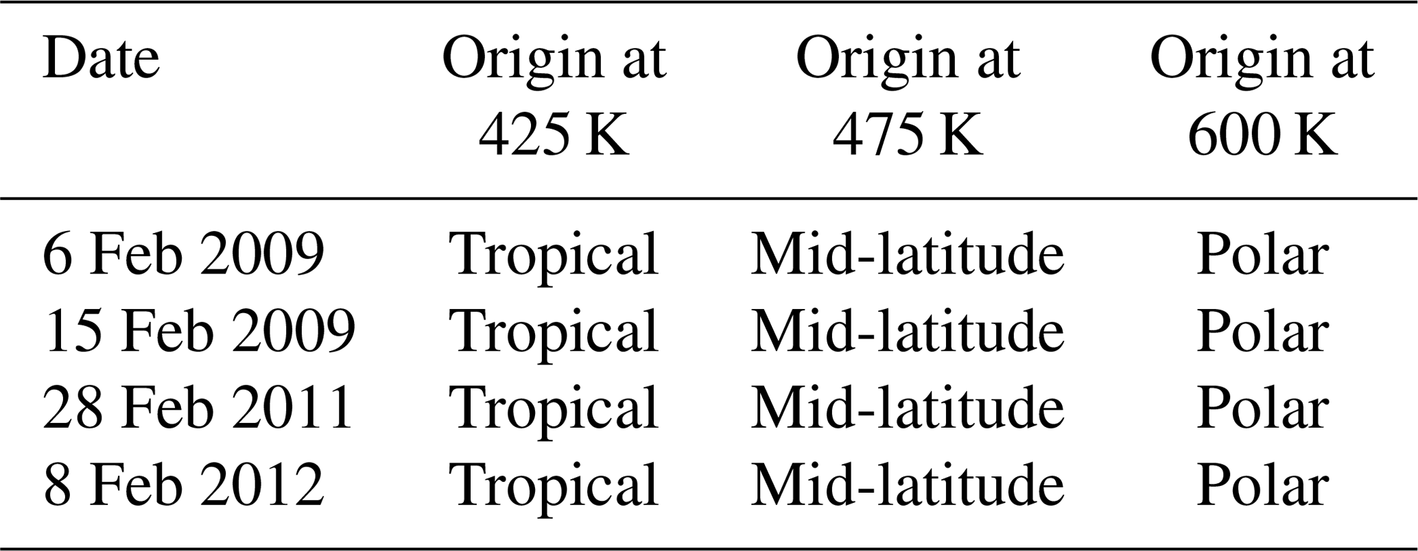
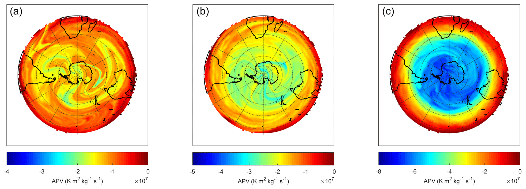
Figure 5Advected potential vorticity (APV) maps from MIMOSA-CHIM at 425 K (a), 475 K (b) and 600 K (c) on 16 January 2012.
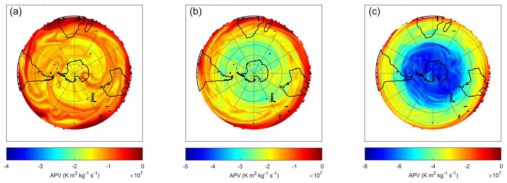
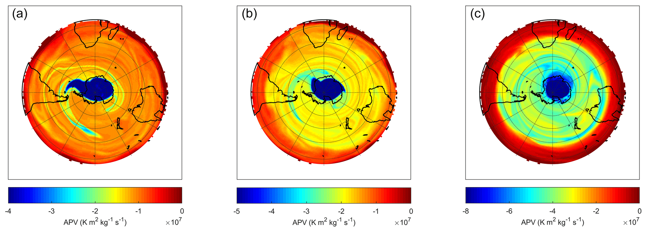
Figure 7APV maps from MIMOSA-CHIM at 435 K (a), 485 K (b) and 600 K (c) on 2 September 2014.
The origin of air masses for low-ozone events during September (Table 5) and the PV maps from MIMOSA-CHIM for the low-ozone event on 2 September 2014 (Fig. 7) show the transport of tropical air masses southward over the study site. During September months there was less mixing of air masses across latitudinal boundaries.
Table 5Origin of ozone-poor air at isentropic levels for low-ozone events in September.
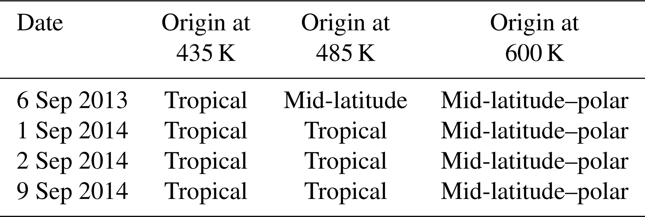
Table 6Origin of ozone-poor air at isentropic levels for low-ozone events in November.
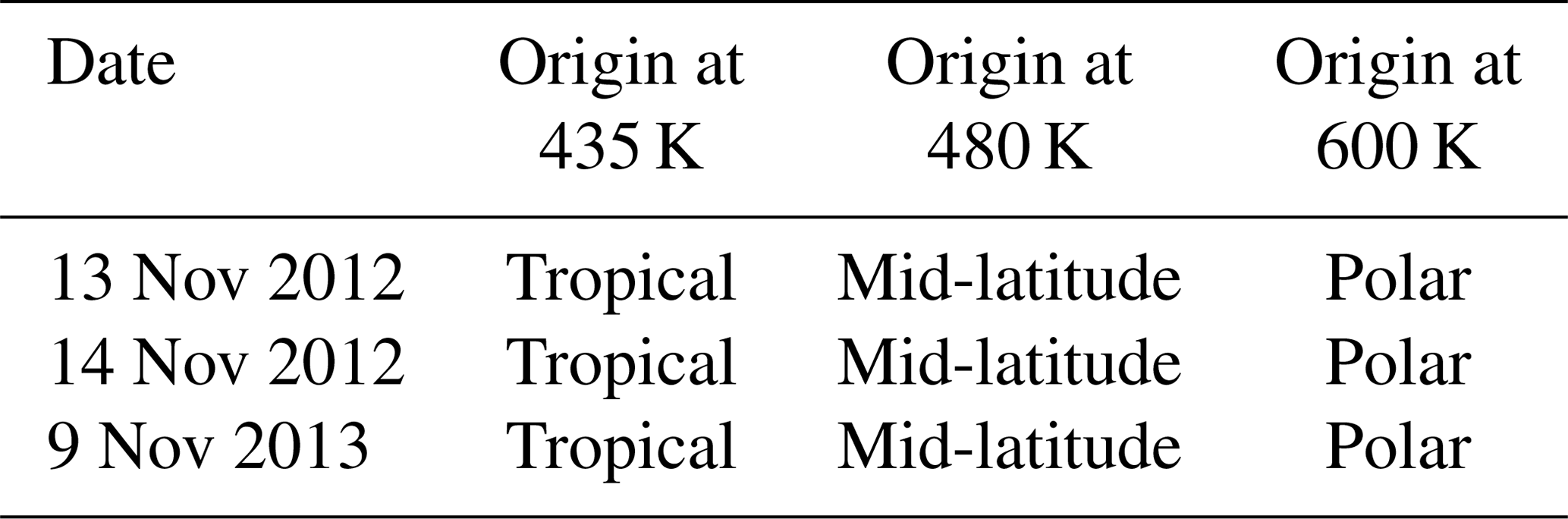
The origin of air masses for low-ozone events in November (Table 6) shows that at 600 K polar air masses do affect the study site, but the ozone hole is no longer present over Antarctica. The PV maps from MIMOSA-CHIM for the low-ozone event on 14 November 2012 (Fig. 8) best demonstrate the situation for November months.
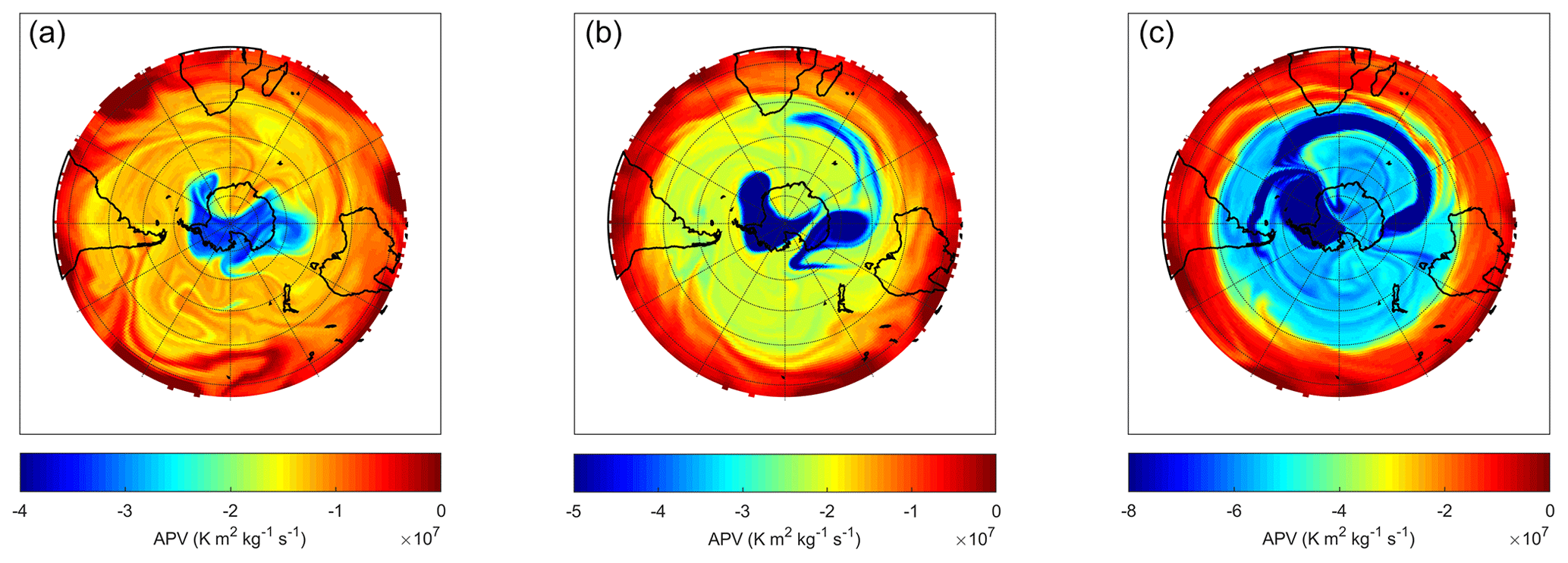
Figure 8APV maps from MIMOSA-CHIM at 435 K (a), 485 K (b) and 600 K (c) on 14 November 2012.
The PV maps from MIMOSA-CHIM suggest that the Antarctic polar vortex air masses with low-ozone levels have a limited effect on the ozone levels over Cape Point, South Africa. Instead, the study site is largely influenced by ozone-poor air masses from sub-tropical regions. The effect of these sub-tropical air masses on ozone concentrations is dependent on isentropic level and time of year. In fact, it is well known that Rossby planetary waves are generated due to the development of synoptic disturbances in the troposphere during winter and spring seasons. They propagate vertically through to the stratospheric layers when the zonal winds are westerly (Charney and Drazin, 1961; Leovy et al., 1985). Moreover, as reported by many authors, gravity and Rossby planetary waves are involved in isentropic transport across the subtropical barrier. Portafaix et al. (2003) studied the southern subtropical barrier by using MIMOSA-CHIM model advected PV maps, together with a numerical tool developed by LACy (Reunion University) named DyBaL (Dynamical Barrier Localisation) based on Nakamura formalism (Nakamura, 1996). They showed that the southern subtropical barrier is usually located around 25–30∘ S but has an increasing variability during winter and spring. Moreover, using MIMOSA-CHIM-adverted PV fields (Bencherif et al., 2007, 2003) showed that exchange processes between the stratospheric tropical reservoir and mid-latitudes are episodic and take place through the subtropical barrier due to planetary wave-breaking inducing increases or decreases in ozone at tropical and subtropical locations depending on the isentropic levels. It is known that atmospheric ozone over South Africa is mainly impacted by dynamical factors (Bodeker et al., 2002). Another dynamical factor that influences ozone over the study area is stratospheric–tropospheric exchanges, which mostly influence SCO levels. One or a combination of these dynamical factors likely result in low-ozone levels over Cape Point.
This study evaluated the anti-correlation between ground-based solar UV-B radiation and satellite ozone observations based on clear-sky days at Cape Point, South Africa. The study further investigated whether the break-up of the Antarctic ozone hole during spring–summer has an impact on the ozone concentrations over the study area and, as a result, affects solar UV-B radiation levels.
The solar UV-B climatology for Cape Point as well as the climatologies of TOC and SCO followed the expected annual cycle for the Southern Hemisphere. The determination of clear-sky days proved to be reliable in identifying cloudy days. The clear-sky tests removed approximately 87 % of days that were affected by cloud cover. At Cape Point, at SZA 25∘, exponential goodness-of-fit R2 values of 0.45 and 0.53 for TOC and SCO, respectively, were found. An average RAF value of 0.59 was found across all SZAs.
Our results from the MIMOSA-CHIM model imply that the break-up of the Antarctic polar vortex has a limited influence on the SCO concentrations over Cape Point. The study site was affected to some extent by Antarctic polar air masses during November months, predominately at 600 K. During September low-ozone events, there was less exchange of air masses between latitudes compared to other months and the study site was mostly under the influence of mid-latitude air masses. The study site seems to be more frequently affected by air masses from the tropical regions, especially in the lower stratosphere. Further, the influence of tropical air masses on the study site is larger during January and February months. During low-SCO events in September and November, the recorded UVI levels were ∼20 % above the climatological monthly mean.
The relationship between atmospheric ozone and solar UV-B radiation is well understood around the world. The impact of the Antarctic ozone hole on atmospheric ozone concentrations over South Africa is less well understood. Our study showed instances when the Antarctic ozone hole seems to have a limited effect on ozone concentrations over Cape Point but also showed the effect of tropical air masses on ozone levels at Cape Point.
The solar UV-B radiation data are available from the South African Weather Service on request. The total ozone column (https://aura.gsfc.nasa.gov/omi.html) and stratospheric column ozone (https://mls.jpl.nasa.gov/) data are available online from the sources as stated in the paper (Bhartia, 2012, Schwartz et al., 2017).
JDP and CYW conceived and designed the experiments, JDP performed the experiments, and JDP and CYW analysed the data. JMC assisted with data conversion. JVA, HB and NB contributed to data analysis and interpretation. JDP and CYW wrote the paper. All authors contributed towards the preparation of the paper.
The authors declare that they have no conflict of interest.
The authors would like to thank the South African Weather Service for
providing solar UV-B radiation data and cloud cover data. The authors
acknowledge the use of Total Ozone Column data from the Ozone Monitoring
Instrument (OMI) and Stratospheric Column Ozone data from the Microwave Limb
Sounder (MLS). The following persons are thanked for the various inputs into
this project: Greg Bodeker of Bodeker Scientific, funded by the New
Zealand Deep South National Science Challenge; Richard McKenzie, National
Institute of Water and Atmospheric Research, New Zealand; and Liesl Dyson,
University of Pretoria. The University of Reunion Island is thanked for the
provision of the MIMOSA-CHIM model and the CCUR team for the use of the
TITAN supercomputer. The SA–French ARSAIO (Atmospheric Research in Southern
Africa and Indian Ocean) and PHC-Protea programmes are also thanked for support for research
visits at the University of Reunion. This study was funded in part by the
South African Medical Research Council as well as the National Research
Foundation of South Africa to grant-holder Caradee Y. Wright.
Edited by: Petr Pisoft
Reviewed by: three anonymous referees
Abarca, J. F., Casiccia, C. C., and Zamorano, F. D.: Increase in sunburns and photosensitivity disorders at the edge of the Antarctic ozone hole, Southern Chile 1986–2000, J. Am. Acad. Dermatol., 46, 193–199, https://doi.org/10.1067/mjd.2002.118556, 2002.
Ajtić, J., Connor, B. J., Lawrence, B. N., Bodeker, G. E., Hoppel, K. W., Rosenfield, J. E., and Heuff, D. N.: Dilution of the Antarctic ozone hole into the southern midlatitudes, J. Geophys. Res., 109, D17107, https://doi.org/10.1029/2003JD004500, 2004.
Bais, A. F., Mckenzie, R. L., Bernhard, G., Aucamp, P. J., llysa, M., Madronich, S., and Tourpali, K.: Ozone depletion and climate change: Impacts on UV radiation, Photochem. Photobiol. Sci., 14, 19–52, https://doi.org/10.1039/c4pp90032d, 2015.
Balis, D., Kroon, M., Koukouli, M. E., Brinksma, E. J., Labow, G., Veefkind, J. P., and McPeters, R. D.: Validation of Ozone Monitoring Instrument total ozone column measurements using Brewer and Dobson spectrophotometer ground-based observations, J. Geophys. Res., 112, D24S46, https://doi.org/10.1029/2007JD008796, 2007.
Bandoro, J., Solomon, S., Donohoe, A., Thompson, D. W., and Santer, B. D.: Influences of the Antarctic Ozone Hole on Southern Hemispheric Summer Climate Change, J. Clim., 27, 6245–6264, https://doi.org/10.1175/JCLI-D-13-00698.1, 2014.
Barsby, J. and Diab, R. D.: Total ozone and synoptic weather relationships over southern Africa and surrounding oceans, J. Geophys. Res., 100, 3023–3032, https://doi.org/10.1029/94JD01987, 1995.
Bencherif, H., Portafaix, T., Baray, J. L., Morel, B., Baldy, S., Leveau, J., Hauchecorne, A., Keckhut, K., Moorgawa, A., Michaelis, M. M., and Diab, R.: LIDAR observations of lower stratospheric aerosols over South Africa linked to large scale transport across the southern subtropical barrier, J. Atmos. Sol.-Terr. Phy., 65, 707–715, 2003.
Bencherif, H., Amraoui, L. E., Semane, N., Massart, S., Vidyaranya Charyulu, D., Hauchecorne, A., and Peuch, V.: Examination of the 2002 major warming in the southen hemisphere using ground-based and Odin/SMR assimilated data: Stratospheric ozone distributions and tropic/mid-latitude exchange, Can. J. Phys., 85, 1287–1300, https://doi.org/10.1139/P07-143, 2007.
Bencherif, H., El Amraoui, L., Kirgis, G., Leclair De Bellevue, J., Hauchecorne, A., Mzé, N., Portafaix, T., Pazmino, A., and Goutail, F.: Analysis of a rapid increase of stratospheric ozone during late austral summer 2008 over Kerguelen (49.4∘ S, 70.3∘ E), Atmos. Chem. Phys., 11, 363–373, https://doi.org/10.5194/acp-11-363-2011, 2011.
Bhartia, P. K.: OMI/Aura Ozone (O3) Total Column Daily L2 Global Gridded 0.25∘ × 0.25∘ V3, , Goddard Earth Sciences Data and Information Services Center (GES DISC), https://doi.org/10.5067/Aura/OMI/DATA2025 (last access: 15 April 2017), 2012.
Bodeker, G.E. and McKenzie, R. L.: An algorithm for inferring surface UV irradiance including cloud effects, J. Appl. Meteor., 35, 1860–1877, 1996.
Bodeker, G. E. and Scourfield, M. W.: Estimated past and future variability in UV radiation in South Africa based on trends in total ozone, S. Afr. J. Sci., 94, 24–32, 1998.
Bodeker, G. E., Struthers, H., and Connor, B. J.: Dynamical containment of Antarctic ozone depletion, Geophys. Res. Lett., 29, 7 pp., https://doi.org/10.1029/2001GL014206, 2002.
Booth, C. R. and Madronich, S.: Radiation Amplification Factors: Improved formulation accounts for large increases in ultraviolet radiation associated with Antarctic ozone depletion, in: Ultraviolet Radiation in Antarctica: Measurements and Biological Effects, 62, Washington, D. C., American Geophysical Union, https://doi.org/10.1029/AR062p0039, 1994.
Brönnimann, S., Jacques-Coper, M., Rozanov, E., Fischer, A. M., Morgenstern, O., Zeng, G., Akiyoshi, H., and Yamashita, Y.: Tropical circulation and precipitation response to ozone depletion and recovery, Environ. Res. Lett., 12, 064011, https://doi.org/10.1088/1748-9326/aa7416, 2017.
Cadet, J.-M., Benchrif, H., Portafaix, T., Lamy, K., Ncongwane, K., Coetzee, G. J., and Wright, C. Y.: Comparison of Ground-Based and Satellite-Derived Solar UV Index Levels at Six South African Sites, Int. J. Env. Res. Pub. He., 14, 1384, https://doi.org/10.3390/ijerph14111384, 2017.
Charney, J. G. and Drazin, P. G.: Propagation of planetary-scale distrubances from the lower into the upper atmosphere, J. Geophys Res., 66, 83–109, 1961.
Climate Prediction Center Internet Team: Cold and warm episodes by season, http://www.cpc.ncep.noaa.gov/products/analysis_monitoring/ensostuff/ensoyears.shtml, last access: 30 August 2017.
de Laat, A., van der A, R. J., Allaart, M. F., van Weele, M., Benitez, G. C., Casiccia, C., Paes Leme, N. M., Quel, E., Salvador, J., and Wolfram, E.: Extreme sunbathing: Three weeks of small total O3 columns and high UV radiation over the southern tip of South America during the 2009 Antartci O3 hole season, Geophys. Res. Lett., 37, L14805, https://doi.org/10.1029/2010GL043699, 2010.
Diab, R., Barsby, J., Bodeker, G., Scourfield, M., and Salter, L.: Satellite observations of total ozone above South Africa, S. Afr. Geogr. J., 74, 13–18, 1992.
Diffey, B. L.: Sources and measurement of ultraviolet radiation, Methods, 28, 4–13, 2002.
Fahey, D. W. and Hegglin, M. L.: Twenty Questions and Answers About the Ozone Layer: 2010 Update, in: Scientific Assesment of Ozone depletion: 2010, Geneva: World Meteorological Organisation, 2011.
Farman, J. C., Gardinier, B. G., and Shanklin, J. D.: Large losses of total ozone in Antarctica reveal seasonal CIO/NO interaction, Nature, 315 207–209, 1985.
Gies, P., Klekociuk, A., Tully, M., Henderson, S., Javorniczky, J., King, K., Lemus-Deschamps, L., and Makin, J.: Low ozone over southern Australia in August 2011 and its imapct on solar ultraviolet radiation levels, Photochem. Photobiol., 89, 984–994, 2013.
Guarnieri, R. A., Padilha, L. F., Guarnieri, F. L., Echer, E., Makita, K., Pinheiro, D. K., Schuch, A. M. P., Boeira, L. S., and Schuch, N. J.: A study of the anticorrelations between ozone and UV-B radiation using linear and exponential fits in southern Brazil, Adv. Space Res., 34, 764–768, 2004.
Hauchecorne, A., Godin, S., Marchand, M., Hesse, B., and Souprayen, C.: Quantification of the transport of chemical constituents from the polar vortex to midlatitudes in the lower stratosphere using the high-resolution advection model MIMOSA and effective diffusivity, J. Geophys. Res., 107, D208289, https://doi.org/10.1029/2001JD000491, 2002.
Hazarika, N.: Correlation and Data Transformations, availibe at: https://blog.majestic.com/case-studies/correlation-data-transformations/ (last access: 30 August 2018), 2013.
Herman, J. R. and McKenzie, R. L.: Ultraviolet radiation at the Earth's surface, in: Scientific Assesment of ozone depletion: 1998, World Meteorological Organisation, 1998.
Holton, J. R. and Hakim, G. J. (Fith Eds.): Circulation, Vorticity and potential vorticity, in: An Introduction to dynamic meteorology Oxford, Academic Press, 2013.
Huang, G., Liu, X., Chance, K., Yang, K., and Cai, Z.: Validation of 10-year SAO OMI ozone profile (PROFOZ) product using Aura MLS measurements, Atmos. Meas. Tech., 11, 17–32, https://doi.org/10.5194/amt-11-17-2018, 2018.
Jiang, Y. B., Froidevaux, L., Lambert, A., Livesey, N. J., Read, W. G., Waters, J. W., Bojkov, B., Leblanc, T., McDermid, I. S., Godin-Beekmann, S., Filipiak, M. J., Harwood, R. S., Fuller, R. A., Daffer, W. H., Drouin, B. J., Cofield, R. E., Cuddy, D. T., Jarnot, R. F., Knosp, B. W., Perun, V. S., Schwartz, M. J., Snyder, W. V., Stek, P. C., Thurstans, R. P., Wagner, P. A., Allaart, M., Andersen, S. B., Bodeker, G., Calpini, B., Claude, H., Coetzee, G.,Davies, J., De Backer, H., Dier, H., Fujiwara, M., Johnson, B., Kelder, H., Leme, N. P., König-Langlo, G., Kyro, E., Laneve, G., Fook, L. S., Merrill, J., Morris, G., Newchurch, M., Oltmans, S., Parrondos, M. C., Posny, F., Schmidlin, F., Skrivankova, P., Stubi, R., Tarasick, D., Thompson, A., Thouret, V., Viatte, P., Vömel, H., von Der Gathen, P., Yela, M., and Zablocki, G.: Validation of Aura Microwave Limb Sounder Ozone by ozonesonde and lidar measurements, J. Geophys. Res., 112, D24S34, https://doi.org/10.1029/2007JD008776, 2007.
Kalicharran, S., Diab, R. D., and Sokolic, F.: Trends in total ozone over southern African stations between 1979 and 1991, Geophys. Res. Lett., 20, 2877–2880, https://doi.org/10.1029/93GL03427, 1993.
Kuttippurath, J., Lefèvre, F., Pommereau, J.-P., Roscoe, H. K., Goutail, F., Pazmiño, A., and Shanklin, J. D.: Antarctic ozone loss in 1979–2010: first sign of ozone recovery, Atmos. Chem. Phys., 13, 1625–1635, https://doi.org/10.5194/acp-13-1625-2013, 2013.
Kuttippurath, J., Godin-Beekmann, S., Lefèvre, F., Santee, M. L., Froidevaux, L., and Hauchecorne, A.: Variability in Antarctic ozone loss in the last decade (2004–2013): high-resolution simulations compared to Aura MLS observations, Atmos. Chem. Phys., 15, 10385–10397, https://doi.org/10.5194/acp-15-10385-2015, 2015.
Lefèvre, F., Brasseur, G. P., Folkins, I., Smith, A. K., and Simon, P: Chemistry of the 199–1992 stratospheric winter: three-dimensional model simulations, J. Geophys. Res., 99, 8183–8195, 1994.
Leovy, C. B., Sun, C. R., Hitchman, M. H., Remsberg, E. E., Russel, J. M., Gordley, L. L., and Lyiak, L. V.: Transport of ozone in the middle stratosphere: evidence for planetary wave breaking, J. Atmos. Sci., 42, 230–244, 1985.
Levelt, P. F., Hilsenrath, E., Leppelmeier, G. W., van den Oord, G. H., Bhartia, P. K., Tamminen, J., and Veefkind, J. P.: Science Objectives of the ozone monitoring instrument, IEEE T. Geosci. Remote Sens., 44, 1199–1208, https://doi.org/10.1109/TGRS.2006.872336, 2006.
Livesey, N. J., Read, W. G., Wagner, P. A., Froidevaux, L., Lambert, A., Manney, G. L., Millan, L. F., Pumphrey, H. C., Santee, M. L., Schwartz, M. J., Wang, S., Fuller, R. A., Jarnot, R. F., Knosp, B. W., and Martinez, E.: The earth observing system (EOS) Aura microwave limb sounder (MLS) Version 4.2xlevel 2 data quality and description document, available at: https://mls.jpl.nasa.gov/data/v4-2_data_quality_document.pdf, last access: 8 May 2017.
Lucas, R. M. and Ponsonby, A.-L.: Ultraviolet radiation and health: friend and foe, Med. J. Australia, 11, 594–598, 2002.
Marchand, M. S., Godin, A., Hauchecorne, A., Lefèvre, F., Bekki, S., and Chipperfield, M.: Influence of polar ozone loss on northern midlatitude regions estimated by a high-resolution chemistry transport model during winter 1999/2000, J. Geophys. Res., 108, https://doi.org/10.1029/2001JD000906, 2003.
Massen, F.: Computing the Radiation Amplification Factor RAF using a sudden dip in Total Ozone Column measured at Diekirch, Luxembourg, https://doi.org/10.13140/RG.2.1.2911.0644, 2013.
McKenzie, R., Connor, B., and Bodeker, G.: Increased summertime UV radiation in New Zealand in response to ozone loss, Science, 285, 1709–1711, 1999.
McKenzie, R. L., Matthews, W. A., and Johnston, P. V.: The relationship between Erythemal UV and ozone derived from spectral irradiance measurements, Geophys. Res. Lett., 18, 2269–2272, https://doi.org/10.1029/91GL02786, 1991.
McKenzie, R. L., Bodeker, G. E., Keep, D. J., and Kotkamp, M.: UV Radiation in New Zealand: North-to-South differences between two sites, and relationship to other latitudes, Weath. Clim., 16, 17–26, 1996.
McPeters, R. D., Frith, S., and Labow, G. J.: OMI total column ozone: extending the long-term data record, Atmos. Meas. Tech., 8, 4845–4850, https://doi.org/10.5194/amt-8-4845-2015, 2015.
Paul, J., Fortuin, F., and Kelder, H.: An ozone climatology based on ozonesonde and satellite measurements, J. Geophys. Res., 103, 709–734, https://doi.org/10.1029/1998JD200008, 1998.
Portafaix, T., Morel, B., Bencherif, H., and Baldy, S.: Fine-scale study of a thick stratospheric ozone lamina at the edge of the southern subtropical barrier, J. Geophys. Res., 108, D64196, https://doi.org/10.1029/2002JD002741, 2003.
Reda, I. and Andreas, A.: NREL's Solar Position Algorithm (SPA), availible at: https://www.nrel.gov/midc/spa/ (last access: 15 August 2017), 2008.
Schuch, A. P., dos Santos, M. B., Lipinski, V. M., Vaz Peres, L., dos Santos, C. P., Cechin, S. Z., Schuch, N. J., Pinheiro, D. K., and da Silva Loreto, E. L.: Identification o finfluential eventsconcerning the Antarctic ozone hole over southern Brazil and the biological effects induced by UVB and UVA radiation in an endemic treefrog species, Ecotox. Environ. Safety, 118, 190–198, https://doi.org/10.1016/j.ecoenv.2015.04.029, 2015.
Schwartz, M., Froidevaux, L., Livesey, N., and Read, W.: MLS/Aura Level 2 Ozone (O3) Mixing Ratio V004, Greenbelt, MD, USA, Goddard Earth Sciences Data and Information Services Center (GES DISC), https://doi.org/10.5067/Aura/MLS/DATA2017 (last access: 8 May 2017), 2015.
Seckmeyer, G., Bais, A., Bernhard, G., Blumthaler, M., Booth, C. R., Lantz, K., and Webb, A.: A Instruments to MeasureSolar Ultraviolet Radiation. Part 2: Broadband Instruments Measuring Erythemally Weighted Solar Irradiance, Geneva, Switzerland, World Meteorological Organization (WMO), 2005.
Semane, N., Bencherif, H., Morel, B., Hauchecorne, A., and Diab, R. D.: An unusual stratospheric ozone decrease in the Southern Hemisphere subtropics linked to isentropic air-mass transport as observed over Irene (25.5∘ S, 28.1∘ E) in mid-May 2002, Atmos. Chem. Phys., 6, 1927–1936, https://doi.org/10.5194/acp-6-1927-2006, 2006.
Serrano, A., Antón, M., Cancillo, M. L., and García, J. A.: Proposal of a new erythemal UV radiation amplification factor, Atmos. Chem. Phys. Discuss., 8, 1089–1111, https://doi.org/10.5194/acpd-8-1089-2008, 2008.
Sivakumar, V. and Ogunniyi, J.: Ozone climatology and variablity over Irene, South Africa detrermined by ground based and satellite observations. Part 1: Vertical variations in the troposphere and stratopshere, Atmosfera, 30, 337–353, 2017.
Slemr, F., Brunke, E. G., Labuschagne, C., and Ebinghaus, R.: Total gaseous mercury concentrations at the Cape Point GAW station and their seasonality, Geophys. Res. Lett., 35, L11807, https://doi.org/10.1029/2008GL033741, 2008.
Solarlight: Model 501 UVB Radiometer, availible at: http://solarlight.com/wp-content/uploads/2015/01/Meters_Model-501-.pdf (last access: 3 September 2016), 2014.
Tripathi, O. P., Godin-Beekmann, S., Lefévre, F., Pazmiño, A., Hauchecorne, A., Chipperfield, M., Feng, W., Millard, G., Rex, M., Streibel, M., and Von der Gathen, P.: Comparison of polar ozone loss rates simulated by one-dimensional and three-dimensional models with match observations in recent Antarctic and Arctic winters, J. Geophys. Res., 112, D12307, https://doi.org/10.1029/2006JD008370, 2007.
WMO: Scientific Asessment of Ozone Depletion: 2010, Global Ozone Research and Monitoring Project- Report No52, Geneva, Switzerland, 2011.
WHO: Ultraviolet radiation and the INTERSUN Programme: http://www.who.int/uv/uv_and_health/en/, last access: 25 January 2017.
Wolfram, E. A., Salvador, J., Orte, F., D'Elia, R., Godin-Beekmann, S., Kuttippurath, J., Pazmiño, A., Goutail, F., Casiccia, C., Zamorano, F., Paes Leme, N., and Quel, E. J.: The unusual persistence of an ozone hole over a southern mid-latitude station during the Antarctic spring 2009: a multi-instrument study, Ann. Geophys., 30, 1435–1449, https://doi.org/10.5194/angeo-30-1435-2012, 2012.
Wright, C. Y., Coetzee, G., and Ncongwane, K.: Ambient solar UV radiation and seasonal trends in potential sunburn risk among schoolchilren in South Africa, S. Afr. J. Child Health, 5, 33–38, 2011.
Zempila, M.-M., van Geffen, J. H. G. M., Taylor, M., Fountoulakis, I., Koukouli, M.-E., van Weele, M., van der A, R. J., Bais, A., Meleti, C., and Balis, D.: TEMIS UV product validation using NILU-UV ground-based measurements in Thessaloniki, Greece, Atmos. Chem. Phys., 17, 7157–7174, https://doi.org/10.5194/acp-17-7157-2017, 2017.