Research on small-scale structures of ice particle density and electron density in the mesopause region

The formation of ice particle density irregularities with a meter scale in the mesopause region is explored in this paper by developing a growth and motion model of ice particles based on the motion equation of a variable mass object. The growth of particles by water vapor adsorption and the action of gravity and the neutral drag force on particles are considered in the model. The evolution of the radius, velocity, and number density of ice particles is then investigated by solving the growth and motion model numerically. For certain nucleus radii, it is found that the velocity of particles can be reversed at a particular height, leading to a local gathering of particles near the boundary layer, which then forms small-scale ice particle density structures. The spatial scale of the density structures can be affected by vertical wind speed, water vapor density, and altitude, and it remains stable as long as these environmental parameters do not change. The influence of the stable small-scale structures on electron and ion density is further calculated by a charging model, which considers the production, loss, and transport of electrons and ions, along with dynamic particle charging processes. Results show that the electron density is anti-correlated to the charged ice particle density and ion density for particles with radii of 11 nm or less due to plasma attachment by particles and plasma diffusion. This finding is in accordance with most rocket observations. The small-scale electron density structures created by small-scale ice particle density irregularities can produce the polar mesosphere summer echo (PMSE) phenomenon.

1 Introduction

Polar mesosphere summer echoes (PMSEs) are strong radar echoes from the polar mesopause in summer (Rapp and Lübken, 2004). One of the features of the PMSEs is that the spectral widths of echoes are much narrower than that of incoherent scatter due to the Brownian movement of electrons (Röttger, et al., 1988, 1990). It has been proposed that the PMSEs are caused by radar waves coherently scattered by irregularities in the refractive index, which are mainly determined by electron density (Rapp and Lübken, 2004). The efficient scattering occurs when the spatial scale of electron density structures is half of the radar wavelength, which is called the Bragg scale. The scale is approximately 3 m for typical VHF radars (Rapp and Lübken, 2004). In the ECT02 rocket campaign (Lübken et al., 1998), a sounding rocket with electron probes detected electron density irregularities in the order of meters during a simultaneous observation of the PMSEs, providing a compelling argument that small-scale electron density structures can indeed create strong radar echoes.

A large amount of research indicates that small-scale ice particle density irregularities in the PMSE region play a key role in creating and maintaining small-scale structures of electron density (Chen and Scales, 2005; Lie-Svendsen et al., 2003; Mahmoudian and Scales, 2013; Rapp and Lübken, 2003; Scales and Ganguli, 2004). Markus Rapp and Franz-Josef Lübken investigated electron diffusion in the vicinity of charged particles (Rapp and Lübken, 2003). They developed coupled diffusion equations for electrons, charged aerosol particles, and positive ions subject to the initial condition of anti-correlated perturbations in charged aerosol and electron distributions. The results illustrate that the perturbations of electron density are anti-correlated to that of the negatively charged aerosol particles and positive ions. Lie-Svendsen et al. studied the plasma response to imposed small-scale aerosol particle density perturbations (Lie-Svendsen et al., 2003). The results were consistent with the solution provided by Markus Rapp's model, in which particle density structures in the order of a few meters could lead to small-scale electron density perturbations due to electron attachment and ambipolar diffusion.

In the work mentioned above, aerosol particle density profiles were directly set as specific small-scale structures such as Gaussian, hyperbolic tangent, or sinusoidal. However, the formation mechanism of the small-scale particle density structures can contribute to a more comprehensive understanding of the PMSE phenomenon and is neglected in such studies. Kopnin et al. used dust acoustic solitons to explain the localized structures of the charged dust particles in the PMSE region (Kopnin et al., 2004), but the spatial scales of the obtained structures were much smaller than the observed scale and wavelength of VHF radar. Therefore, the formation mechanism of small-scale structures in the PMSE region remains not clear.

In the polar mesopause region, neutral airflow moves upward (Garcia and Solomon, 1985). The ice particles are subject to upward neutral drag force and downward gravity, and they grow by absorbing water vapor simultaneously. In addition, the size of initial condensation nuclei has a certain distribution. These factors can cause complex trajectories of ice particles and result in an inhomogeneous distribution of particle number density, leading to small-scale structures of electron density. This may be an important mechanism that can produce a PMSE phenomenon. However, few studies have explored the formation process of small-scale ice particle structures from the perspective of ice particle growth and movement.

A particle growth and motion model is thus developed in this paper to describe the evolution of the ice particle radius, velocity, and density distribution in the mesopause region. The growth of particles is based on the collision and adsorption process of condensation nuclei and water vapor. The particle movement is predominantly controlled by the gravity and the neutral drag force. With the obtained ice particle density structures, the corresponding electron and ion densities are calculated based on a charging model, which includes the continuity equations for ice particles with various charges and ions, the momentum equation for ions and electrons, and the quasi-neutral condition.

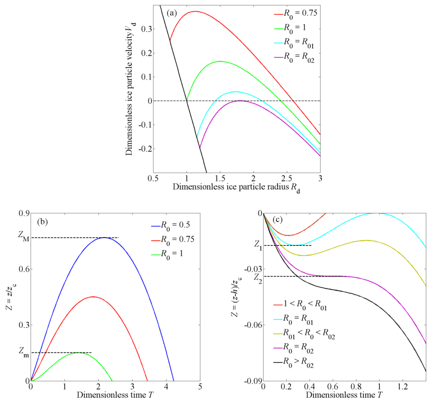
Figure 1 (a) Dependence of the ice particle velocity on radius for different initial nucleus radii. The black solid line $V_{d\mathrm{0}}=\mathrm{1}-R_{\mathrm{0}}$ represents the relation between the initial particle velocity and the initial particle radius. (b) Movement curves of ice particles near the lower boundary. (c) Movement curves of ice particles near the upper boundary.

2 Model

Equations for the growth and motion model of condensation nuclei and the charging model of ice particles are detailed in this section.

The simulation is carried out at a summer polar mesopause region between 80 and 90 km, where the water vapor carried by neutral gas is determined to move upwards at a constant speed (Garcia and Solomon, 1985). It is assumed that micrometeorites enter the study region at a certain flux from the upper boundary, and volcanic ash or particles ejected by the aircraft rise into the region from the lower boundary. These grains serve as condensation cores. When the temperature is lower than the frost point (Körner and Sonnemann, 2001), water vapor molecules that touch the surface of the grains due to thermal motion can easily condense into ice. In this process, condensation cores become ice particles and continue to grow. In this article, only the growth, motion, and charging process of particles inside the condensation layer are discussed, and only the vertical transport of particles and plasma is considered as the horizontal gradients of transport parameters are much smaller comparatively (Lie-Svendsen et al., 2003).

For growing ice particles, the dynamic equation for a variable mass object is applied.

$$\begin{array}{}\text{(1)}& m_{\mathrm{d}}{\displaystyle \frac{\mathrm{d}{u}_{\mathrm{d}}}{\mathrm{d}t}}+(u_{\mathrm{d}}-u){\displaystyle \frac{\mathrm{d}{m}_{\mathrm{d}}}{\mathrm{d}t}}=m_{\mathrm{d}}g-{\mathit{\mu }}_{\mathrm{dn}}{m}_{\mathrm{d}}(u_{\mathrm{d}}-u)+q_{\mathrm{d}}E,\end{array}$$

where m_d, u_d, and q_d are the mass, velocity, and charge of ice particles, respectively, u is the velocity of neutral gas, g is gravitational acceleration, μ_dn is the collision frequency between ice particles and gas, and E is the electric field. The electric force has a trivial effect on the motion of ice particles because the charge–mass ratio of particles is usually very small (Jensen and Thomas, 1988; Pfaff et al., 2001). The inertial term is also negligible as its magnitude is much smaller than gravity (Garcia and Solomon, 1985).

The water vapor is supersaturated in the polar mesopause region (Lübken, 1999), and it is assumed that the size of condensation nuclei is larger than the condensation critical size, so stable growth of ice particles will continue when water molecules collide with particles during thermal motion. Ignoring reverse processes such as sublimation, the mass change rate of ice particles is

$$\begin{array}{}\text{(2)}& {\displaystyle \frac{\mathrm{d}{m}_{\mathrm{d}}}{\mathrm{d}t}}={\mathit{\mu }}_{\mathrm{wd}}{m}_{\mathrm{w}}.\end{array}$$

The collision frequency between water vapor and ice particles is ${\mathit{\mu }}_{\mathrm{wd}}=n_{\mathrm{w}}\mathit{\pi }{r}_{\mathrm{d}}^{\mathrm{2}}{v}_{\mathrm{w}}$ based on the hard-sphere collision model (Lieberman and Lichtenberg, 2005), in which m_w, n_w, and v_w are the mass, number density, and thermal velocity of water molecules, respectively.

The collision frequency between air molecules and ice particles in the neutral drag force term is (Schunk, 1977)

$$\begin{array}{}\text{(3)}& {\mathit{\mu }}_{\mathrm{dn}}={\displaystyle \frac{\mathrm{8}}{\mathrm{3}\sqrt{\mathit{\pi }}}}{\displaystyle \frac{n_{\mathrm{n}}{m}_{\mathrm{n}}}{m_{\mathrm{d}}+m_{\mathrm{n}}}}\sqrt{{\displaystyle \frac{\mathrm{2}{k}_{\mathrm{B}}{T}_{\mathrm{g}}(m_{\mathrm{d}}+m_{\mathrm{n}})}{m_{\mathrm{d}}{m}_{\mathrm{n}}}}}\mathit{\pi }{\left(r_{\mathrm{d}}+r_{\mathrm{n}}\right)}^{\mathrm{2}},\end{array}$$

where n_n, m_n, and r_n are the number density, mean molecule mass, and effective radius of neutral molecule, respectively, and T_g is the gas temperature. The neutral molecule mass m_n is assumed to be 28.96 m_u, in which m_u is the proton mass.

According to Eq. (1) the velocity of ice particles is obtained as

$$\begin{array}{}\text{(4)}& u_{\mathrm{d}}=u+{\displaystyle \frac{m_{\mathrm{d}}}{{\mathit{\mu }}_{\mathrm{dn}}{m}_{\mathrm{d}}+{\mathit{\mu }}_{\mathrm{wd}}{m}_{\mathrm{w}}}}g.\end{array}$$

On the basis that n_w≪n_n (Seele and Hartogh, 1999), m_w≪ m_d, m_n≪ m_d, r_n≪r_d, v_n∼v_w and taking vertical up to be the positive direction, the velocity of ice particles is simplified as

$$\begin{array}{}\text{(5)}& u_{\mathrm{d}}=u-g/{\mathit{\mu }}_{\mathrm{dn}}.\end{array}$$

Ice particles are composed of condensation nuclei and the attached ice. The mass of a single ice particle is

$$\begin{array}{}\text{(6)}& m_{\mathrm{d}}={\displaystyle \frac{\mathrm{4}}{\mathrm{3}}}\mathit{\pi }{r}_{\mathrm{0}}^{\mathrm{3}}{\mathit{\rho }}_{\mathrm{0}}+{\displaystyle \frac{\mathrm{4}}{\mathrm{3}}}\mathit{\pi }(r_{\mathrm{d}}^{\mathrm{3}}-r_{\mathrm{0}}^{\mathrm{3}}){\mathit{\rho }}_{\mathrm{d}},\end{array}$$

where r₀ and ρ₀ are the initial radius and mass density of condensation nuclei and ρ_d is the mass density of ice.

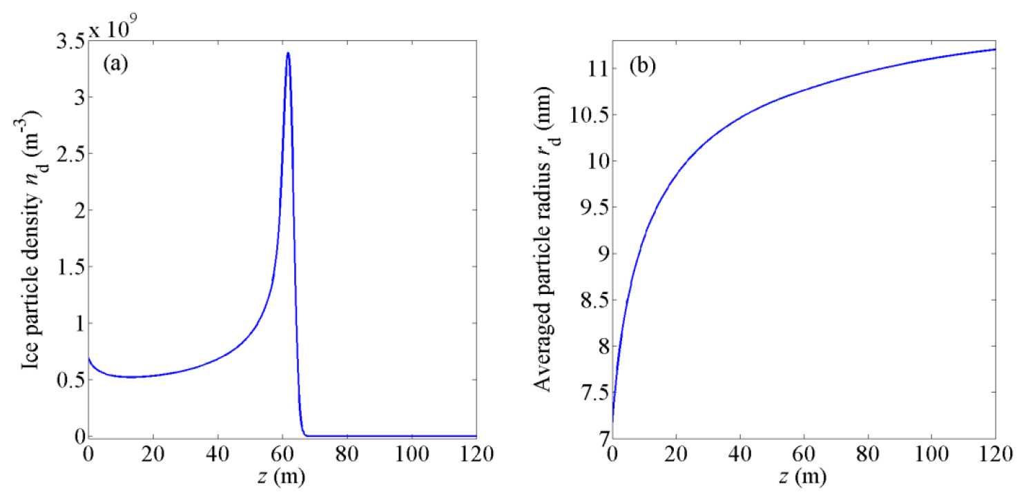
Figure 2 Distribution of (a) ice particle density and (b) averaged particle radius near the lower boundary of the condensation layer.

Based on the expressions of m_d and μ_dn, the relation between ice particle velocity and radius is

$$\begin{array}{}\text{(7)}& u_{\mathrm{d}}=u-{\displaystyle \frac{g}{n_{\mathrm{n}}{m}_{\mathrm{n}}{v}_{\mathrm{n}}}}[{\mathit{\rho }}_{\mathrm{d}}{r}_{\mathrm{d}}+({\mathit{\rho }}_{\mathrm{0}}-{\mathit{\rho }}_{\mathrm{d}}\left){\displaystyle \frac{r_{\mathrm{0}}^{\mathrm{3}}}{r_{\mathrm{d}}^{\mathrm{2}}}}\right].\end{array}$$

At the boundaries of the condensation region r_d=r₀, the initial velocity of condensation nuclei is

$$\begin{array}{}\text{(8)}& u_{\mathrm{d}\mathrm{0}}=u(\mathrm{1}-r_{\mathrm{0}}/r_{\mathrm{c}}),\end{array}$$

where r_c is the critical radius of

$$\begin{array}{}\text{(9)}& r_{\mathrm{c}}=n_{\mathrm{n}}{m}_{\mathrm{n}}{v}_{\mathrm{n}}u/\left(g{\mathit{\rho }}_{\mathrm{0}}\right).\end{array}$$

When the radius of condensation nuclei is r₀>r_c, gravity is larger than the neutral drag force of v_d0<0 and particles move downwards. Otherwise, particles move upwards.

Based on the relation between m_d and r_d, the change rate of ice particle radius is

$$\begin{array}{}\text{(10)}& {\displaystyle \frac{\mathrm{d}{r}_{\mathrm{d}}}{\mathrm{d}t}}={\displaystyle \frac{\mathrm{1}}{\mathrm{4}}}{\displaystyle \frac{n_{\mathrm{w}}{m}_{\mathrm{w}}{v}_{\mathrm{w}}}{{\mathit{\rho }}_{\mathrm{d}}}}=c.\end{array}$$

It can be clearly observed that the ice particle radius increases linearly with time.

$$\begin{array}{}\text{(11)}& r_{\mathrm{d}}=r_{\mathrm{0}}+ct\end{array}$$

The particle trajectory can then be obtained by the following integral:

$$\begin{array}{}\text{(12)}& z-z_{\mathrm{0}}={\int }_{\mathrm{0}}^t{u}_{\mathrm{d}}\mathrm{d}t=c^{-\mathrm{1}}{\int }_{r_{\mathrm{0}}}^{r_{\mathrm{d}}}{u}_{\mathrm{d}}\mathrm{d}{r}_{\mathrm{d}},\end{array}$$

where z₀ is the reference height where condensation nuclei enter the studied region. In this work z₀=0 is set at the lower boundary, and z₀=h is set at the upper boundary, where h is the distance between the two boundaries.

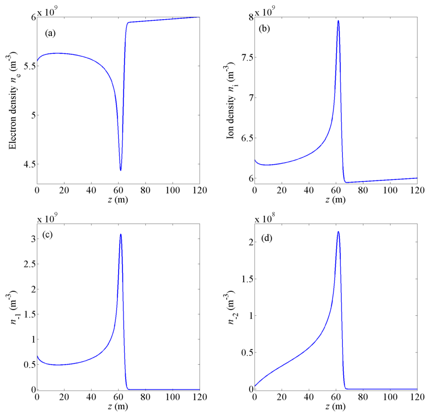
Figure 3 Number density distribution of (a) electrons n_e, (b) ions n_i, (c) particles carrying one negative charge n₋₁, and (d) particles carrying two negative charges n₋₂ near the lower boundary of the condensation layer at t=1000 s.

It is assumed that the condensation nucleus radius ranging from r_0 min to r_0 max has a certain distribution function f(r₀). The density of condensation nuclei with a radius in the small range is $r_{\mathrm{0}}\to r_{\mathrm{0}}+\mathrm{d}{r}_{\mathrm{0}}$ is dn(r₀)=f(r₀)dr₀, and their velocity is u_d0. When these particles arrive at height z, their radius increases to r_d(r₀,z), the corresponding number density turns into dn(r₀, z), and the velocity becomes u_d(r₀, z) =u_d[r₀, r_d(r₀,z)]. According to the particle conservation law,

$$\begin{array}{}\text{(13)}& u_{\mathrm{d}\mathrm{0}}\mathrm{d}n\left(r_{\mathrm{0}}\right)=u_{\mathrm{d}}(r_{\mathrm{0}},z)\mathrm{d}n(r_{\mathrm{0}},z).\end{array}$$

The number density of ice particles at height z can then be obtained by

$$\begin{array}{}\text{(14)}& n_{\mathrm{d}}\left(z\right)=\int \mathrm{dn}(r_{\mathrm{0}},z)={\int }_{r_{\mathrm{0}\min }}^{r_{\mathrm{0}\max }}{\displaystyle \frac{u_{\mathrm{d}\mathrm{0}}f\left(r_{\mathrm{0}}\right)}{u_{\mathrm{d}}(r_{\mathrm{0}},z)}}\mathrm{d}{r}_{\mathrm{0}}.\end{array}$$

The averaged ice particle radius at height z is

$$\begin{array}{}\text{(15)}& {\stackrel{\mathrm{‾}}{r}}_{\mathrm{d}}\left(z\right)={\displaystyle \frac{\int r_{\mathrm{d}}\left(z\right)\mathrm{dn}(r_{\mathrm{0}},z)}{n_{\mathrm{d}}\left(z\right)}}.\end{array}$$

By integrating all condensation nucleus radii, a stable distribution of n_d and r_d can be obtained. The particles continue to enter and leave the condensation region, and as long as the external environment does not change, the distribution of particle density and radius will remain unchanged. The influence of these stable n_d and r_d profiles on electron and ion density is then calculated.

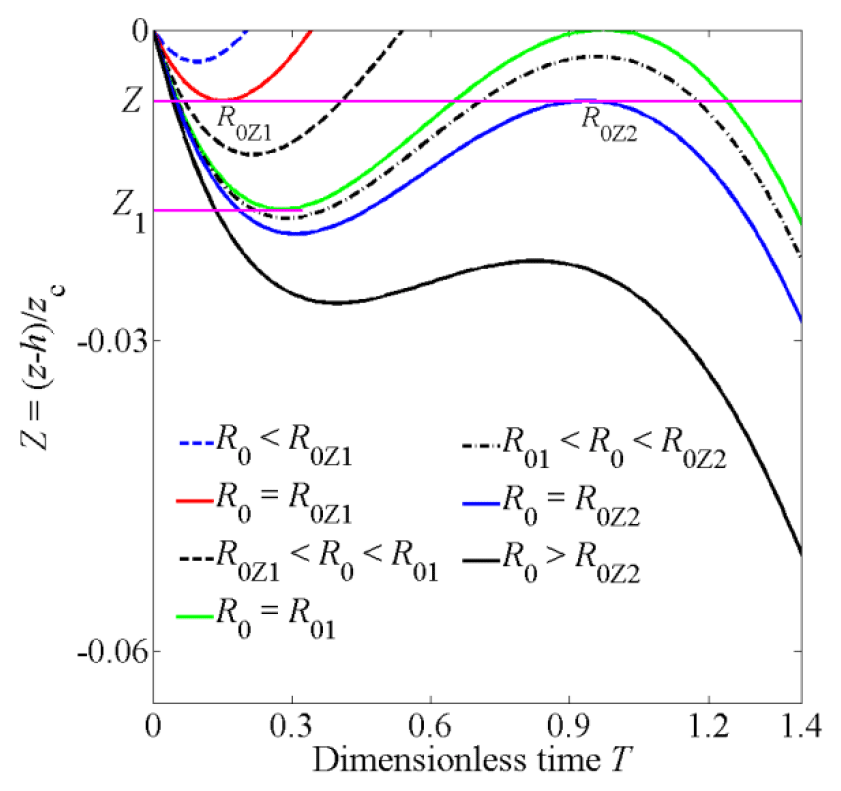
Figure 4 Movement curves of ice particles near the upper boundary. The particles with initial radius R_0Z1 move upward after turning back at the Z height (the red line), and the particles with initial radius R_0Z2 move downward after turning back at Z (the blue line).

Considering ionization, electron–ion recombination, and ion loss on ice particles, the continuity equation of ion density can be written as

$$\begin{array}{}\text{(16)}& {\displaystyle \frac{\partial n_{\mathrm{i}}}{\partial t}}+{\displaystyle \frac{\partial \left(n_{\mathrm{i}}{u}_{\mathrm{i}}\right)}{\partial z}}=Q-\mathit{\alpha }{n}_{\mathrm{i}}{n}_{\mathrm{e}}-D^{+}{n}_{\mathrm{i}}.\end{array}$$

Ignoring gravity, the drift velocity of ions u_i is determined by

$$\begin{array}{}\text{(17)}& u_{\mathrm{i}}={\displaystyle \frac{eE}{m_{\mathrm{i}}{\mathit{\mu }}_{\mathrm{in}}}}-{\displaystyle \frac{k_{\mathrm{B}}{T}_{\mathrm{g}}}{m_{\mathrm{i}}{\mathit{\mu }}_{\mathrm{in}}}}{\displaystyle \frac{\mathrm{1}}{n_{\mathrm{i}}}}{\displaystyle \frac{\partial n_{\mathrm{i}}}{\partial z}}.\end{array}$$

The electric field E is predominantly determined by the electron density gradient because the diffusion coefficient and mobility of electrons are much larger than that of ions.

$$\begin{array}{}\text{(18)}& E=-{\displaystyle \frac{k_{\mathrm{B}}{T}_{\mathrm{g}}}{e}}{\displaystyle \frac{\mathrm{1}}{n_{\mathrm{e}}}}{\displaystyle \frac{\partial n_{\mathrm{e}}}{\partial z}}\end{array}$$

In the typical PMSE layer, there are several kinds of ions carrying one unit positive charge: ${\mathrm{N}}_{\mathrm{2}}^{+}$, ${\mathrm{O}}_{\mathrm{2}}^{+}$, NO⁺, and H⁺(H₂O)_n. As specified by Reid (Reid, 1990), the averaged ion parameters n_i, m_i, and T_g are applied to describe the density, mass, and temperature of ions, respectively, and the averaged ion mass m_i is set as 50 m_u at 85 km altitude. According to the theory of Hill and Bowhill (1977), the ion-neutral collision frequency is

$$\begin{array}{}\text{(19)}& \begin{array}{l}{\mathit{\mu }}_{\mathrm{in}}=\mathrm{2.6}\times {\mathrm{10}}^{-\mathrm{15}}{n}_{\mathrm{n}}\left(\mathrm{0.78}\frac{\mathrm{28}}{M_{\mathrm{i}}+\mathrm{28}}\sqrt{\mathrm{1.74}\frac{M_{\mathrm{i}}+\mathrm{28}}{\mathrm{28}{M}_{\mathrm{i}}}}\right.\\ +\mathrm{0.21}\frac{\mathrm{32}}{M_{\mathrm{i}}+\mathrm{32}}\sqrt{\mathrm{1.57}\frac{M_{\mathrm{i}}+\mathrm{32}}{\mathrm{32}{M}_{\mathrm{i}}}}\\ \left.+\mathrm{0.01}\frac{\mathrm{40}}{M_{\mathrm{i}}+\mathrm{40}}\sqrt{\mathrm{1.64}\frac{M_{\mathrm{i}}+\mathrm{40}}{\mathrm{40}{M}_{\mathrm{i}}}}\right)\end{array},\end{array}$$

where $M_{\mathrm{i}}=m_{\mathrm{i}}/m_u$.

The production rate for ions and electrons Q is chosen to be 3.6×10⁷ m⁻³ s⁻¹, and the electron–ion recombination coefficient α is set as 10⁻¹² m³ s⁻¹ (Lie-Svendsen et al., 2003). The undisturbed density of ions and electrons is $n_{\mathrm{0}}=\mathrm{6}\times {\mathrm{10}}^{\mathrm{9}}$ m⁻³. The loss coefficient of ions on ice particles is $D^{+}=\mathrm{\Sigma }{n}_q{\mathit{\nu }}_{\mathrm{i},q}$, where n_q is the number density of the q-charged ice particles and ν_i,q represents the capture rate of ions by ice particles with q charges. According to the discrete charging model (Robertson and Sternovsky, 2008),

$$\begin{array}{}\text{(20)}& {\mathit{\nu }}_{\mathrm{i},q\le \mathrm{0}}=\mathit{\pi }{r}_{\mathrm{d}}^{\mathrm{2}}{c}_{\mathrm{i}}\left(\mathrm{1}+C_q\sqrt{{\displaystyle \frac{e^{\mathrm{2}}}{\mathrm{16}{\mathit{\epsilon }}_{\mathrm{0}}{k}_{\mathrm{B}}{T}_{\mathrm{g}}{r}_{\mathrm{d}}}}}+D_q{\displaystyle \frac{e^{\mathrm{2}}}{\mathrm{4}\mathit{\pi }{\mathit{\epsilon }}_{\mathrm{0}}{k}_{\mathrm{B}}{T}_{\mathrm{g}}{r}_{\mathrm{d}}}}\right).\end{array}$$

The particle radius r_d used here is the averaged radius [U+F8E5] r_d, which is obtained using Eq. (15). The ion thermal velocity is c_i= (8k_BT_g∕π m_i); k_B is the Boltzmann constant; and ε₀ is the permittivity of a vacuum. The C_q and D_q are provided in Table 1 in the work of Robertson and Sternovsky (Robertson and Sternovsky, 2008), and the corresponding capture rates of electrons by ice particles (Robertson and Sternovsky, 2008) are denoted as

$$\begin{array}{}\text{(21)}& {\displaystyle }{\mathit{\nu }}_{\mathrm{e},q\ge \mathrm{0}}=\mathit{\pi }{r}_{\mathrm{d}}^{\mathrm{2}}{c}_{\mathrm{e}}\left(\mathrm{1}+C_q\sqrt{{\displaystyle \frac{e^{\mathrm{2}}}{\mathrm{16}{\mathit{\epsilon }}_{\mathrm{0}}{k}_{\mathrm{B}}{T}_{\mathrm{g}}{r}_{\mathrm{d}}}}}+D_q{\displaystyle \frac{e^{\mathrm{2}}}{\mathrm{4}\mathit{\pi }{\mathit{\epsilon }}_{\mathrm{0}}{k}_{\mathrm{B}}{T}_{\mathrm{g}}{r}_{\mathrm{d}}}}\right),\text{(22)}& {\displaystyle }\begin{array}{rl}& {\mathit{\nu }}_{\mathrm{e},q<\mathrm{0}}=\mathit{\pi }{r}_{\mathrm{d}}^{\mathrm{2}}{\mathit{\gamma }}^{\mathrm{2}}{c}_{\mathrm{e}}\\ & \exp \left[-{\displaystyle \frac{\left|q\right|e^{\mathrm{2}}}{\mathrm{4}\mathit{\pi }{\mathit{\epsilon }}_{\mathrm{0}}{k}_{\mathrm{B}}{T}_{\mathrm{g}}{r}_{\mathrm{d}}\mathit{\gamma }}}\left(\mathrm{1}-{\displaystyle \frac{\mathrm{1}}{\mathrm{2}\mathit{\gamma }\left({\mathit{\gamma }}^{\mathrm{2}}-\mathrm{1}\right)\left|q\right|}}\right)\right].\end{array}\end{array}$$

The thermal velocity of electrons c_e= (8k_BT_g∕πm_e) and the value of γ for each q is referenced from Natanson's paper (Natanson, 1960).

Although the distribution of total particle density n_d=Σn_q reaches a stable state under the action of gravity and neutral drag force, the number density of the q-charged ice particles n_q is dynamic in the charging process. The continuity equation of q-charged ice particle density is

$$\begin{array}{}\text{(23)}& \begin{array}{rl}{\displaystyle \frac{\partial n_q}{\partial t}}& =n_{q+\mathrm{1}}{\mathit{\nu }}_{\mathrm{e},q+\mathrm{1}}{n}_{\mathrm{e}}+n_{q-\mathrm{1}}{\mathit{\nu }}_{\mathrm{i},q-\mathrm{1}}{n}_{\mathrm{i}}\\ & -\left(n_q{\mathit{\nu }}_{\mathrm{e},q}{n}_{\mathrm{e}}+n_q{\mathit{\nu }}_{\mathrm{i},q}{n}_{\mathrm{i}}\right)\end{array}.\end{array}$$

According to previous research (Lie-Svendsen et al., 2003; Rapp and Lübken, 2001), it is assumed that a single particle carries two negative charges at the most, i.e., $q=-\mathrm{2}$, −1, 0, and +1 in this study.

According to typical parameters in the PMSE region (Rapp and Lübken, 2001), the plasma Debye length λ_D is estimated to be approximately 9 mm, which is much smaller than the vertical spatial scale of the PMSE layer. Thus, the dusty plasma satisfies the quasi-neutral condition.

$$\begin{array}{}\text{(24)}& n_{\mathrm{i}}+{\sum }_{q}q{n}_q=n_{\mathrm{e}}\end{array}$$

For simplicity, dimensionless parameters will be used in subsequent discussion.

$$\begin{array}{rl}& V_{\mathrm{d}}=v_{\mathrm{d}}/u,\mathit{\rho }={\mathit{\rho }}_{\mathrm{d}}/{\mathit{\rho }}_{\mathrm{0}},R_{\mathrm{0}}=r_{\mathrm{0}}/r_{\mathrm{c}},R_{\mathrm{d}}=r_{\mathrm{d}}/r_{\mathrm{c}}\\ & T=t/t_{\mathrm{c}},Z=(z-z_{\mathrm{0}})/z_{\mathrm{c}},\end{array}$$

where $t_{\mathrm{c}}=r_{\mathrm{c}}/c$, which represents the time it takes for ice particles to grow from r_d to r_d+r_c, and z_c=ut_c is the distance that neutral wind moves during the time t_c.

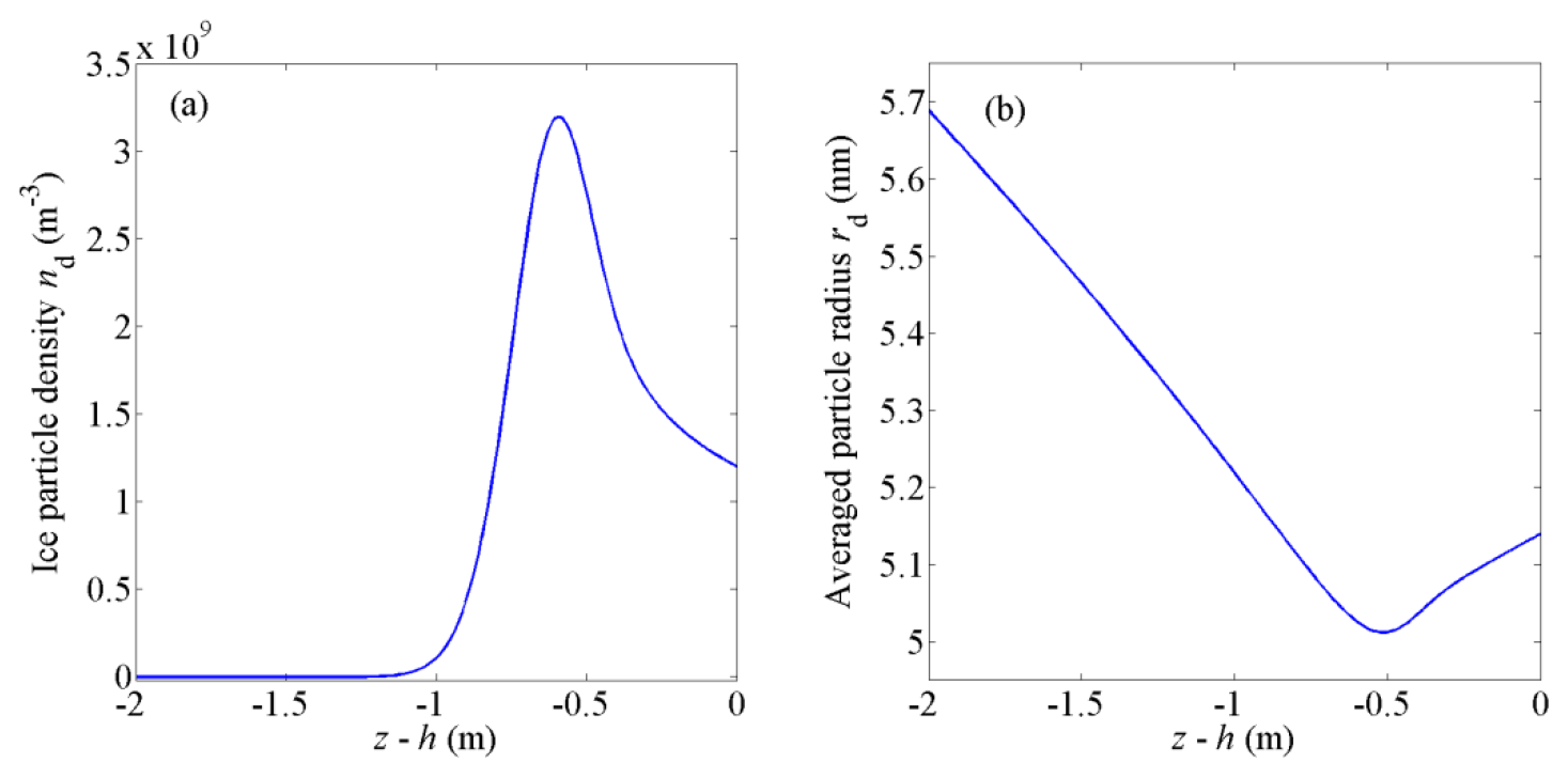
Figure 5 The distribution of (a) ice particle density and (b) the averaged particle radius near the upper boundary of the condensation layer.

Figure 6 The number density distribution of (a) electrons, (b) ions, (c) particles carrying one negative charge, and (d) particles carrying two negative charges near the upper boundary of the condensation layer at t=1000 s.

The expression of dimensionless ice particle velocity is

$$\begin{array}{}\text{(25)}& V_{\mathrm{d}}=\mathrm{1}-\mathit{\rho }{R}_{\mathrm{d}}-(\mathrm{1}-\mathit{\rho }){\displaystyle \frac{R_{\mathrm{0}}^{\mathrm{3}}}{R_{\mathrm{d}}^{\mathrm{2}}}}.\end{array}$$

The expressions of the dimensionless position coordinate of particles based on T and R_d are

$$\begin{array}{}\text{(26)}& {\displaystyle }Z(R_{\mathrm{0}},T)=T-{\displaystyle \frac{\mathrm{1}}{\mathrm{2}}}\mathit{\rho }T(T+\mathrm{2}{R}_{\mathrm{0}})-(\mathrm{1}-\mathit{\rho })R_{\mathrm{0}}^{\mathrm{2}}{\displaystyle \frac{T}{T+R_{\mathrm{0}}}},\text{(27)}& {\displaystyle }\begin{array}{rl}Z(R_{\mathrm{0}},R_{\mathrm{d}})& =R_{\mathrm{d}}-R_{\mathrm{0}}-{\displaystyle \frac{\mathrm{1}}{\mathrm{2}}}\mathit{\rho }(R_{\mathrm{d}}^{\mathrm{2}}-R_{\mathrm{0}}^{\mathrm{2}})\\ & +(\mathrm{1}-\mathit{\rho })R_{\mathrm{0}}^{\mathrm{3}}\left({\displaystyle \frac{\mathrm{1}}{R_{\mathrm{d}}}}-{\displaystyle \frac{\mathrm{1}}{R_{\mathrm{0}}}}\right).\end{array}\end{array}$$

The dimensionless number density and radius distribution of ice particles are

$$\begin{array}{}\text{(28)}& {\displaystyle }{n}_{\mathrm{d}}\left(Z\right)=n_{\mathrm{0}}{\int }_{R_{\mathrm{0}min}}^{R_{\mathrm{0}max}}{\displaystyle \frac{V_{\mathrm{d}\mathrm{0}}F\left(R_{\mathrm{0}}\right)}{V_{\mathrm{d}}[R_{\mathrm{0}},R_{\mathrm{d}}(R_{\mathrm{0}},Z\left)\right]}}\mathrm{d}{R}_{\mathrm{0}},\text{(29)}& {\displaystyle }{\stackrel{\mathrm{‾}}{R}}_{\mathrm{d}}\left(Z\right)={\displaystyle \frac{n_{\mathrm{0}}}{n_{\mathrm{d}}\left(Z\right)}}{\int }_{R_{\mathrm{0}min}}^{R_{\mathrm{0}max}}{\displaystyle \frac{R_{\mathrm{d}}\left(Z\right)V_{\mathrm{d}\mathrm{0}}F\left(R_{\mathrm{0}}\right)}{V_{\mathrm{d}}[R_{\mathrm{0}},R_{\mathrm{d}}(R_{\mathrm{0}},Z\left)\right]}}\mathrm{d}{R}_{\mathrm{0}},\end{array}$$

where n₀ is the density of condensation cores at the boundary, and it is assumed to be 5×10⁸ m⁻³ (Bardeen et al., 2008). The normalized radius distribution function F(R₀) satisfies ${\int }_{R_{\mathrm{0}min}}^{R_{\mathrm{0}max}}F\left(R_{\mathrm{0}}\right)\mathrm{d}{R}_{\mathrm{0}}=\mathrm{1}$.

In subsequent calculations, parameters are taken in the atmospheric environment at an altitude of 85 km. The number density of neutrals is $n_n=\mathrm{2.3}\times {\mathrm{10}}^{\mathrm{20}}$ m⁻³ (Hill et al., 1999); the number density of water vapor is $n_{\mathrm{w}}=\mathrm{2.5}\times {\mathrm{10}}^{\mathrm{14}}$ m⁻³ (Seele and Hartogh, 1999); the temperature is T_g=150 K; the mass density of ice is ${\mathit{\rho }}_{\mathrm{d}}=\mathrm{1}\times {\mathrm{10}}^{\mathrm{3}}$ kg m⁻³; the velocity of neutral wind is u=3 cm s⁻¹ (Garcia and Solomon, 1985); the mass density of condensation nucleus is ${\mathit{\rho }}_{\mathrm{0}}=\mathrm{2.7}\times {\mathrm{10}}^{\mathrm{3}}$ kg m⁻³; and the growth rate of ice particles is $c\approx \mathrm{7.8}\times {\mathrm{10}}^{-\mathrm{4}}$ nm s⁻¹. In this work, we only consider the growth and movement of condensation nuclei which fall from the upper boundary with the initial radius r₀>r_c and rise from the lower boundary with r₀≤r_c.

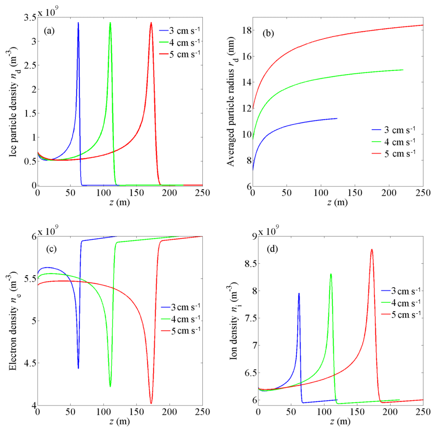
Figure 7 The distribution of (a) ice particle density, (b) the averaged particle radius, (c) electron density, and (d) ion density for various vertical wind speeds near the lower boundary of the condensation layer.

3 Results and discussion

3.1 Speed and trajectory of ice particles

The relation between V_d and R_d is illustrated in Fig. 1a, which shows that condensation nuclei with an initial radius R₀≤1 rise into the PMSE region through the lower boundary, while particles with R₀>1 fall into the region from the upper boundary. At the beginning, the upward-moving particles accelerate and the downward particles decelerate due to $\partial V_{\mathrm{d}}/\partial R_{\mathrm{d}}=\mathrm{2}-\mathrm{3}\mathit{\rho }\mathit{>}\mathrm{0}$ when R_d=R₀. Later, with the increase of R_d, $\partial V_{\mathrm{d}}/\partial R_{\mathrm{d}}\mathit{<}\mathrm{0}$, all particles will move with a downward acceleration, which makes them eventually move downward.

Figure 1b shows the movement curves of ice particles near the lower boundary. These particles, with an initial radius R₀≤1 will rise into the condensation layer. With the collection of ice, the grains become larger and heavier, leading to their deceleration. The grains will then accelerate downward until they leave the condensation layer from the lower boundary. All particles rising from the lower boundary will retrace in the range Z_m<Z<Z_M. Z_m is the maximum height that particles with an initial radius R₀=1 can reach, and Z_M is the maximum height that particles with an initial radius $R_{\mathrm{0}}=R_{\mathrm{0}min}=\mathrm{0.5}$ can reach. Based on above parameters, Z_m=0.1512 and Z_M=0.7682.

Figure 8 The distribution of (a) ice particle density, (b) the averaged particle radius, (c) electron density, and (d) ion density for various vertical wind speeds near the upper boundary of the condensation layer.

Figure 1c shows the movement curves of ice particles near the upper boundary, which can be sorted by the value of R₀. For 1<R₀<R₀₁, the neutral drag force increases faster than gravity as the particles fall. The particles decelerate to zero speed, retrace upward, and then leave the condensation layer from the upper boundary. For R₀=R₀₁, the particles retrace at the height Z=Z₁, then they arrive at Z=0 with exactly zero velocity, and the particles move back into the condensation layer again. For R₀₁<R₀<R₀₂, the particles retrace upward in the range of Z₂<Z<Z₁ and move downward again before they reach the upper boundary. For R₀=R₀₂, the particles decelerate downward until zero speed at Z=Z₂. Here, the acceleration happens to be zero. Then the gravity exceeds the drag force, and the particles accelerate downward. For R₀>R₀₂, the particles continue moving down after entering the condensation layer. According to the above parameters, R₀₁ and R₀₂ are solved as 1.1519 and 1.19705, respectively.

It can be observed in Fig. 1 that the particles with a certain initial radius will move up and down several times near the boundary; namely, ice particles will accumulate at that region and form some kind of small-scale density structure.

Figure 9 The distribution of (a) ice particle density, (b) the averaged particle radius, (c) electron density, and (d) ion density for various water vapor densities near the lower boundary of the condensation layer.

Figure 10 The distribution of (a) ice particle density, (b) the averaged particle radius, (c) electron density, and (d) ion density for various water vapor densities near the upper boundary of the condensation layer.

3.2 Density and radius distribution of ice particles and their effects on plasma

3.2.1 Near the lower boundary

The density and radius distribution of ice particles near the lower boundary are first solved. As illustrated in Fig. 1b, all ice particles with an initial radius R₀≤1 will pass the range 0<Z<Z_m twice, so they contribute twice to the calculation of particle density. In the height range Z_m<Z<Z_M, only the particles that can reach the Z height will contribute to the density at Z. The density and mean radius of ice particles near the lower boundary are shown below.

$$\begin{array}{}\text{(30)}& {\displaystyle }\begin{array}{rl}{n}_{\mathrm{d}}\left(Z\right)& =n_{\mathrm{0}}{\int }_{\mathrm{0.5}}^{R_{\mathrm{0}Z}}{V}_{\mathrm{d}\mathrm{0}}F\left(R_{\mathrm{0}}\right)\\ & \left[{\displaystyle \frac{\mathrm{1}}{V_{\mathrm{d}\mathrm{1}}(R_{\mathrm{0}},R_{\mathrm{d}\mathrm{1}})}}+{\displaystyle \frac{\mathrm{1}}{\mathrm{|}{V}_{\mathrm{d}\mathrm{2}}(R_{\mathrm{0}},R_{\mathrm{d}\mathrm{2}})\mathrm{|}}}\right]\mathrm{d}{R}_{\mathrm{0}},\end{array}\text{(31)}& {\displaystyle }\begin{array}{rl}{\stackrel{\mathrm{‾}}{R}}_{\mathrm{d}}\left(Z\right)& ={\displaystyle \frac{n_{\mathrm{0}}}{n_{\mathrm{d}}\left(Z\right)}}{\int }_{\mathrm{0.5}}^{R_{\mathrm{0}Z}}{V}_{\mathrm{d}\mathrm{0}}F\left(R_{\mathrm{0}}\right)\\ & \left[{\displaystyle \frac{R_{\mathrm{d}\mathrm{1}}}{V_{\mathrm{d}\mathrm{1}}(R_{\mathrm{0}},R_{\mathrm{d}\mathrm{1}})}}+{\displaystyle \frac{R_{\mathrm{d}\mathrm{2}}}{\left|V_{\mathrm{d}\mathrm{2}}\right(R_{\mathrm{0}},R_{\mathrm{d}\mathrm{2}}\left)\right|}}\right]\mathrm{d}{R}_{\mathrm{0}},\end{array}\end{array}$$

where R_d1 and R_d2 are particle radii when particles pass through the Z height, V_d1 and V_d2 are the corresponding velocities, and the upper limit of integral R_0Z is determined by

$$\begin{array}{}\text{(32)}& R_{\mathrm{0}Z}=\left\{\begin{array}{cc}\mathrm{1}& \text{if}{Z}_{\mathrm{m}}\mathit{<}Z\mathit{<}{Z}_{\mathrm{M}}\\ \text{solution of}\left(Z\left(R_{\mathrm{0}Z},R_{\mathrm{d}}\right)=Z\right)& \text{if}\mathrm{0}\mathit{<}Z\mathit{<}{Z}_{\mathrm{m}}\end{array}\right..\end{array}$$

In this study, the radius distribution function of condensation cores is assumed to be a Gaussian distribution.

$$\begin{array}{}\text{(33)}& F\left(R_{\mathrm{0}}\right)=A\exp \left[-{\left(R_{\mathrm{0}}-R_{\mathrm{00}}\right)}^{\mathrm{2}}/{\mathrm{\Delta }}^{\mathrm{2}}\right],\end{array}$$

where the center of the radius distribution function R₀₀ is chosen to be 0.8, the characteristic width is Δ=0.01, and the corresponding normalized coefficient is A=56.4.

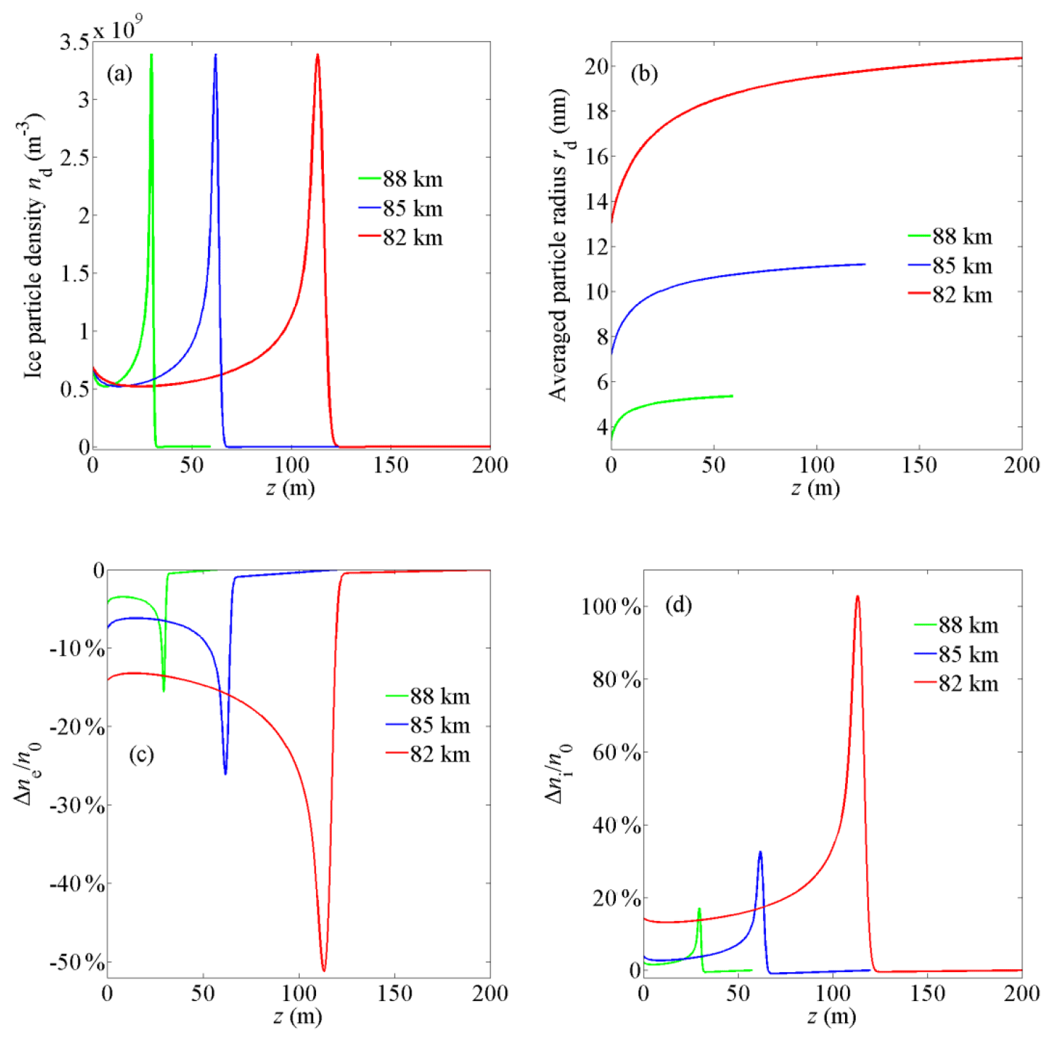
Figure 11 The distribution of (a) ice particle density, (b) the averaged particle radius, (c) the relative change of electron density Δn_e∕n_e, and (d) the relative change of ion density Δn_i∕n_i at various altitudes near the lower boundary of the condensation layer.

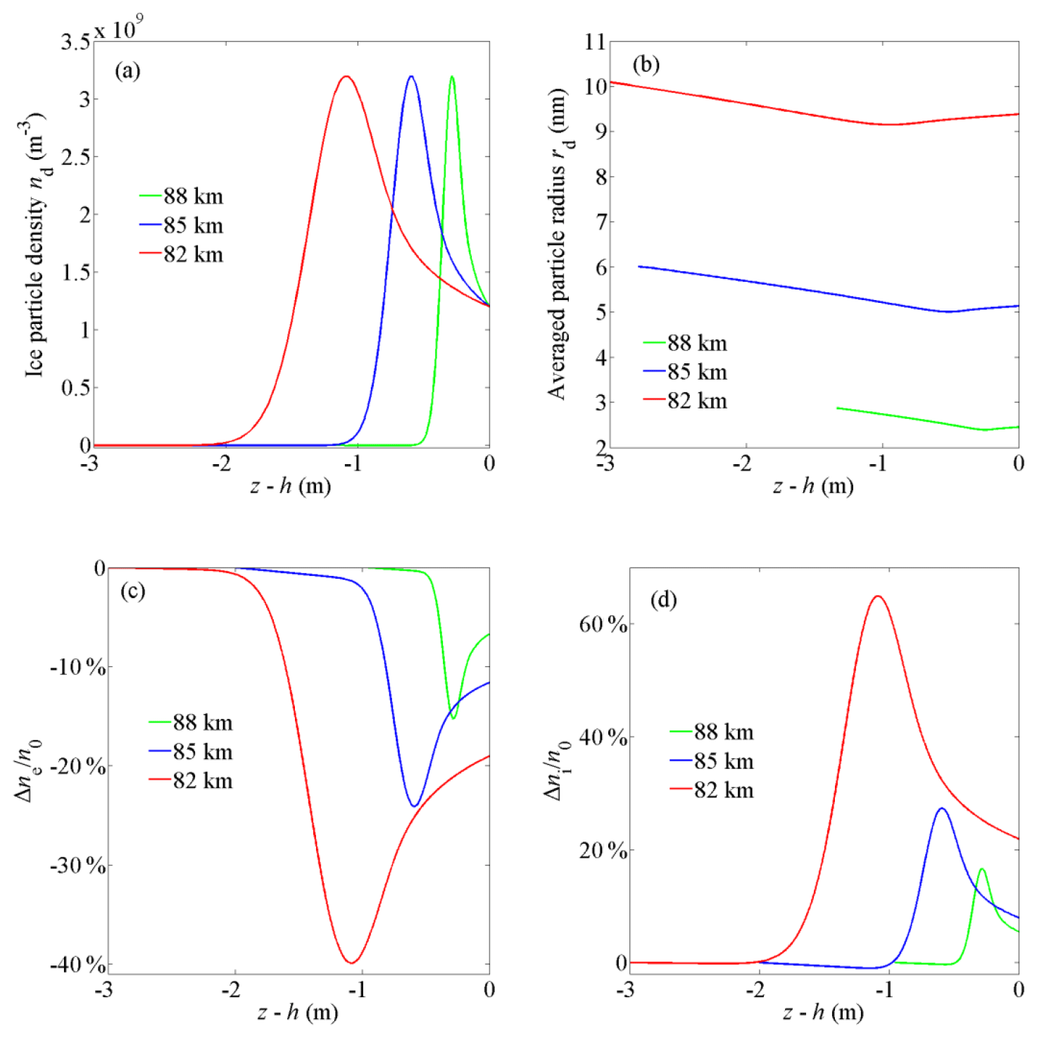
Figure 12 The distribution of (a) ice particle density, (b) the averaged particle radius, (c) the relative change of electron density Δn_e∕n_e, and (d) the relative change of ion density Δn_i∕n_i at various altitudes near the upper boundary of the condensation layer.

The obtained density and mean radius of ice particles near the lower boundary are presented in Fig. 2a and b, respectively. Figure 2a shows that a sharp peak appears in the density distribution of ice particles. The width at the half maximum of the irregularity is about 5 m, which is consistent with the assumed ice particle density structure scale in theoretical work (Lie-Svendsen et al., 2003; Rapp and Lübken, 2003) as well as in the observation by the sounding rocket flight ECT02 in July 1994 (Rapp and Lübken, 2004). In Fig. 2b, it can be observed that the average radius of ice particles increases from 7 to 11 nm with height.

According to the obtained density and average radius of ice particles in Fig. 2a and b, the density distribution of electrons, ions, and charged ice particles is calculated based on the charging model described by Eqs. (16)–(24). At the initial moment of the charging model, all ice particles are assumed to be neutral in order to conduct the calculation more conveniently, as the final distributions of charge are independent from the initial ice particle charge state (Lie-Svendsen et al., 2003). The timescale of electrons collected by negatively charged particles with a radius of 10 nm is approximately 700 s, which is the longest timescale in the charging process. The quasi-steady state of charging can then be obtained after this timescale. Therefore, the calculation is terminated after 1000 s, and the results are illustrated in Fig. 3.

Figure 3a shows that electron density decreases sharply around z=60 m due to adsorption by particles and the reduction of electron density $\mathrm{\Delta }{n}_{\mathrm{e}}\approx (n_{-\mathrm{1}}+\mathrm{2}{n}_{-\mathrm{2}})/\mathrm{2}$, which corresponds to the results under diffusion equilibrium approximations in earlier work (Lie-Svendsen et al., 2003). Ion number density increases sharply around 60 m due to diffusion under the ambipolar electric field. The ambipolar diffusion process of electrons and ions has been described in detail in previous work (Lie-Svendsen et al., 2003). Electron density is anti-correlated to density irregularities of ions and the charged ice particles due to the attachment and diffusion processes. The anti-correlations correspond with rocket observations by the sounding rocket flight SCT-06 in August 1993 (Lie-Svendsen et al., 2003) and the sounding rocket flight ECT02 in July 1994 (Rapp and Lübken, 2004). According to Fig. 3c and d, it can be determined that for particles with radii ranging from 7 to 11 nm, the proportion of particles carrying one negative charge ranges from 97.5 % to 85.1 %, and the value for particles carrying two negative charges is 0.53 %–13.6 %, which is consistent with observations by Havnes et al. (1996) and numerical results by Rapp and Lübken (2001). The density of positively charged particles is less than 1.1×10⁵ m⁻³ and is insignificant in this study.

3.2.2 Near the upper boundary

The parameters of ice particles and plasma near the upper boundary are discussed in this subsection, based on the movement curves of ice particles near the upper boundary, as shown in Fig. 4.

For Z₁<Z<0, particles with an initial radius R_0Z1 and R_0Z2 turn back at Z and move upward and downward separately, as shown in Fig. 4. The values of R_0Z1 and R_0Z2 are determined by the equations $V_{\mathrm{d}}(R_{\mathrm{0}Z},R_{\mathrm{d}})=\mathrm{0}$ and $Z(R_{\mathrm{0}Z},R_{\mathrm{d}})=Z$. The contribution of ice particles to the density distribution near the upper boundary can be classified as follows:

1. R₀<R_0Z1: ice particles cannot reach Z and make no contributions to the number density.

2. R_0Z1<R₀<R₀₁: ice particles pass through Z twice and contribute to n_d(Z) twice. The radius of particles when passing through the Z height can be obtained as R_d31 andR_d32 based on Eq. (27). Their corresponding velocities are calculated respectively as V_d31 and V_d32 based on Eq. (25).

3. R₀₁<R₀<R_0Z2: ice particles pass through Z three times. The corresponding radii and velocities at Z are defined as R_d41, R_d42, and R_d43 andV_d41, V_d42, and V_d43.

4. R₀>R_0Z2: ice particles pass through Z only once, and their radius and velocity are R_d5 and V_d5, respectively.

Substituting these parameters into Eqs. (28) and (29), the density and mean radius of ice particles in the range Z₁<Z<0 are deduced as

$$\begin{array}{}\text{(34)}& {\displaystyle }\begin{array}{ll}{n}_{\mathrm{d}}\left(Z\right)& =n_{\mathrm{0}}{\int }_{R_{\mathrm{0}Z\mathrm{1}}}^{R_{\mathrm{01}}}\mathrm{|}{V}_{\mathrm{d}\mathrm{0}}\mathrm{|}F\left(R_{\mathrm{0}}\right)\\ & \left[\frac{\mathrm{1}}{\mathrm{|}{V}_{\mathrm{d}\mathrm{31}}(R_{\mathrm{0}},R_{\mathrm{d}\mathrm{31}})\mathrm{|}}+\frac{\mathrm{1}}{V_{\mathrm{d}\mathrm{32}}(R_{\mathrm{0}},R_{\mathrm{d}\mathrm{32}})}\right]\mathrm{d}{R}_{\mathrm{0}}\\ & +n_{\mathrm{0}}{\int }_{R_{\mathrm{01}}}^{R_{\mathrm{0}Z\mathrm{2}}}\mathrm{|}{V}_{\mathrm{d}\mathrm{0}}\mathrm{|}F\left(R_{\mathrm{0}}\right)\\ & \left[\frac{\mathrm{1}}{\mathrm{|}{V}_{\mathrm{d}\mathrm{41}}(R_{\mathrm{0}},R_{\mathrm{d}\mathrm{41}})\mathrm{|}}+\frac{\mathrm{1}}{V_{\mathrm{d}\mathrm{42}}(R_{\mathrm{0}},R_{\mathrm{d}\mathrm{42}})}\right.\\ & \left.+\frac{\mathrm{1}}{\mathrm{|}{V}_{\mathrm{d}\mathrm{43}}(R_{\mathrm{0}},R_{\mathrm{d}\mathrm{43}})\mathrm{|}}\right]\mathrm{d}{R}_{\mathrm{0}}\\ & +n_{\mathrm{0}}{\int }_{R_{\mathrm{0}Z\mathrm{2}}}^{R_{\mathrm{0}max}}\frac{\mathrm{|}{V}_{\mathrm{d}\mathrm{0}}\mathrm{|}F\left(R_{\mathrm{0}}\right)}{\mathrm{|}{V}_{\mathrm{d}\mathrm{5}}(R_{\mathrm{0}},R_{\mathrm{d}\mathrm{5}})\mathrm{|}}\mathrm{d}{R}_{\mathrm{0}}\end{array},\text{(35)}& {\displaystyle }\begin{array}{ll}{\stackrel{\mathrm{‾}}{R}}_{\mathrm{d}}\left(Z\right)& =\frac{n_{\mathrm{0}}}{n_{\mathrm{d}}\left(Z\right)}{\int }_{R_{\mathrm{0}Z\mathrm{1}}}^{R_{\mathrm{01}}}\mathrm{|}{V}_{\mathrm{d}\mathrm{0}}\mathrm{|}F\left(R_{\mathrm{0}}\right)\\ & \left[\frac{R_{\mathrm{d}\mathrm{31}}}{\mathrm{|}{V}_{\mathrm{d}\mathrm{31}}(R_{\mathrm{0}},R_{\mathrm{d}\mathrm{31}})\mathrm{|}}+\frac{R_{\mathrm{d}\mathrm{32}}}{V_{\mathrm{d}\mathrm{32}}(R_{\mathrm{0}},R_{\mathrm{d}\mathrm{32}})}\right]\mathrm{d}{R}_{\mathrm{0}}\\ & +\frac{n_{\mathrm{0}}}{n_{\mathrm{d}}\left(Z\right)}{\int }_{R_{\mathrm{01}}}^{R_{\mathrm{0}Z\mathrm{2}}}\mathrm{|}{V}_{\mathrm{d}\mathrm{0}}\mathrm{|}F\left(R_{\mathrm{0}}\right)\\ & \left[\frac{R_{\mathrm{d}\mathrm{41}}}{\mathrm{|}{V}_{\mathrm{d}\mathrm{41}}(R_{\mathrm{0}},R_{\mathrm{d}\mathrm{41}})\mathrm{|}}+\frac{R_{\mathrm{d}\mathrm{42}}}{V_{\mathrm{d}\mathrm{42}}(R_{\mathrm{0}},R_{\mathrm{d}\mathrm{42}})}\right.\\ & \left.+\frac{R_{\mathrm{d}\mathrm{43}}}{\mathrm{|}{V}_{\mathrm{d}\mathrm{43}}(R_{\mathrm{0}},R_{\mathrm{d}\mathrm{43}})\mathrm{|}}\right]\mathrm{d}{R}_{\mathrm{0}}\\ & +\frac{n_{\mathrm{0}}}{n_{\mathrm{d}}\left(Z\right)}{\int }_{R_{\mathrm{0}Z\mathrm{2}}}^{R_{\mathrm{0}max}}\frac{R_{\mathrm{d}\mathrm{5}}\mathrm{|}{V}_{\mathrm{d}\mathrm{0}}\mathrm{|}F\left(R_{\mathrm{0}}\right)}{\mathrm{|}{V}_{\mathrm{d}\mathrm{5}}(R_{\mathrm{0}},R_{\mathrm{d}\mathrm{5}})\mathrm{|}}\mathrm{d}{R}_{\mathrm{0}}\end{array}.\end{array}$$

The center of the radius distribution function is R₀₀=1.08; the characteristic width is Δ=0.01; and the corresponding normalized coefficient is A=56.4.

The ice particle density in the region of Z<Z₁ is close to zero, as only particles with an initial radius R₀≥R₀₁ can arrive at the region, and the number of the particles in this radius range is very low based on the radius distribution function set above.

At the upper boundary, the number density of condensation cores n₀ is set as 5×10⁸ m⁻³, and the maximum radius of condensation cores is $R_{\mathrm{0}max}=\mathrm{1.3}$. The number density and mean radius of ice particles are obtained from Eqs. (34) and (35) and are shown in Fig. 5. The density distribution of electrons, ions, and charged ice particles is then calculated further based on the charging model.

Figure 5a shows that there is a meter scale structure in the distribution of ice particle density, which is consistent with the assumed ice particle density structure scale in previous theoretical work (Lie-Svendsen et al., 2003; Rapp and Lübken, 2003) and rocket observations (Rapp and Lübken, 2004). In addition, the average radius of ice particles is slightly larger than 5 nm (shown in Fig. 5b).

As illustrated in Fig. 6a, compared with ice particle density, there is a similar but anti-correlated structure in the electron density profile because of the adsorption of electrons by particles. Due to ambipolar diffusion, ion density increases in the perturbed region. The reduction of electron density Δn_e and the increment of ion density Δn_i are consistent with the results under diffusion equilibrium approximations: $\mathrm{\Delta }{n}_e\approx \mathrm{\Delta }{n}_{\mathrm{i}}\approx (n_{-\mathrm{1}}+\mathrm{2}{n}_{-\mathrm{2}})/\mathrm{2}$ (Lie-Svendsen et al., 2003). According to Fig. 6c and d, 97 % of the particles carry one negative charge, and few particles carry two negative charges. This is reasonable for particles with a radius slightly larger than 5 nm.

3.3 Influence of the vertical wind speed on the spatial scale of the irregularities

The vertical wind speed is varied from 3 to 5 cm s⁻¹ to investigate the influence of the wind speed on the spatial scale of the irregularities. With all other parameters remaining the same, the numerical results are shown in Figs. 7 and 8. When the wind speed is increased, the spatial scale of the irregularities increases as higher wind speed corresponds to a larger critical particle radius r_c in the growth model (see Eq. 9). This leads to a longer timescale (t_c) and larger spatial scale (z_c) of ice particle growth and movement. In addition, as shown in Fig. 7c and d, with the increase of wind speed, the variation amplitude of electron density and ion density near the lower boundary obviously increases. This is because the averaged radius of the ice particles increases with the extension of the particle growth time (see Fig. 7b), and the particles' influence on the plasma increases. The variation amplitude of electron density and ion density near the upper boundary does not notably change (see Fig. 8c and d) because there is little variation in the averaged radii of the ice particles for different wind speeds, as shown in Fig. 8b.

3.4 Influence of the water vapor density on the spatial scale of the irregularities

Water vapor density can also affect the spatial scale of the particle density structures by modifying the change rate of the particle radius. As illustrated in Figs. 9 and 10, the spatial scale of the irregularities decreases when the water vapor density increases. A larger vapor density results in a higher change rate of the particle radius (see Eq. 10) and a shorter timescale (t_c) of ice particle growth. The particles can then reach the inversion condition more quickly, and the reverse position is closer to the boundary, meaning that the spatial scale of the ice particle density structures becomes shorter.

3.5 Influence of the altitude on the irregularities spatial scale

The effect of the altitude on the spatial scale of the irregularities is explored in this subsection. The altitude mainly affects the neutral gas density n_n, ion composition, ion mass m_i, production rate for plasma Q, electron–ion recombination coefficient α, and plasma density n₀ without ice particles. In addition to 85 km, altitudes of 82 and 88 km are also included as they are near the lower and upper limits of the PMSE region (Lie-Svendsen et al., 2003). According to previous work (Blix, 1999; Lübken, 1999; Rapp and Lübken, 2001), at 82 km, the positive ions are mainly (H₃O)⁺(H₂O)₃ cluster ions with m_i=73 m_u, and other parameters are set as $n_n=\mathrm{4.2}\times {\mathrm{10}}^{\mathrm{20}}$ m⁻³, $Q=\mathrm{6.3}\times {\mathrm{10}}^{\mathrm{7}}$ m⁻³ s⁻¹, $\mathit{\alpha }=\mathrm{7}\times {\mathrm{10}}^{-\mathrm{12}}$ m³ s⁻¹, and $n_{\mathrm{0}}=\mathrm{3}\times {\mathrm{10}}^{\mathrm{9}}$ m⁻³. At 88 km altitude, the positive ions are mainly NO⁺ with m_i=30 m_u, and other parameters are $n_{\mathrm{n}}=\mathrm{1.1}\times {\mathrm{10}}^{\mathrm{20}}$ m⁻³, $Q=\mathrm{6}\times {\mathrm{10}}^{\mathrm{7}}$ m⁻³ s⁻¹, $\mathit{\alpha }=\mathrm{6}\times {\mathrm{10}}^{-\mathrm{13}}$ m³ s⁻¹, and $n_{\mathrm{0}}=\mathrm{1}\times {\mathrm{10}}^{\mathrm{10}}$ m⁻³. The numerical results are provided in Figs. 11 and 12. As the ambient plasma density n₀ varies dramatically at different altitudes, the electron density relative change Δn_e∕n_e and the ion density relative change Δn_i∕n_i are calculated for comparison, where $\mathrm{\Delta }{n}_{\mathrm{e}}=n_{\mathrm{e}}-n_{\mathrm{0}}$ and $\mathrm{\Delta }{n}_{\mathrm{i}}=n_{\mathrm{i}}-n_{\mathrm{0}}$. Figures 11a and 12a show that with the increase in altitude, the spatial scale of the ice particle density irregularities becomes shorter. The reason for this finding is that higher altitudes correspond to a smaller neutral density n_n and critical particle radius r_c (see Eq. 9), which leads to a shorter timescale (t_c) and spatial scale (z_c) of ice particle growth and movement. It is notable that the spatial scale of the electron density irregularities at lower altitudes is longer than that at higher altitudes (see Figs. 11c and 12c). This result is consistent with the explanation provided by Bremer et al. that at lower altitudes the PMSE signals detected by long-wavelength radar (half wavelength of 54 m) are stronger than those detected by short-wavelength radar (half wavelength of 2.8 m) (Bremer et al., 1997). In addition, with the increase of altitude, the relative change amplitude of electron density and ion density decreases significantly because the averaged radius of the ice particles at higher altitudes is smaller, and the influence of ice particles on plasma decreases.

4 Conclusions

In this paper, a growth and motion model of ice particles was developed based on the equation of variable mass object motion in order to explain the formation of ice particle density irregularities with a meter scale in the polar mesopause region. The density profile of ice particles with height was investigated according to the conservation of the particle number. Based on the growth and motion model, small-scale structures of ice particle density were successfully produced. The density distributions of electrons and ions corresponding to the ice particle density distribution were then obtained based on quasi-neutrality and the discrete charging model. The findings are summarized as follows.

The ice particle radius increases linearly with time. However, a complex relation occurs between the velocity and radius of particles due to the variable mass of ice particles and the complicated force operating on them. For a certain radius of the condensation nucleus, ice particles can bounce near the boundary layer, which leads to a local gathering phenomenon of ice particles and the creation of meter scale ice particle density structures. The spatial scale of the density structures can be affected by vertical wind speed, water vapor density, and altitude. The spatial scale increases with the increase of wind speed, and it decreases with the increase of water vapor density and altitude. Small-scale ice particle density irregularities can remain stable if these atmospheric conditions do not change. In the ice particle gathering region, the electron density is anti-correlated to the charged ice particle density and the ion density because of the plasma attachment by ice particles and plasma diffusion. To summarize, small-scale ice particle density irregularities are formed and maintained in the polar mesopause region based on the growth and motion model, and the corresponding small-scale electron density structures are in accordance with most rocket observations.