Comparison of CSES ionospheric RO data with COSMIC measurements

CSES (China Seismo-Electromagnetic Satellite) is a newly launched electric-magnetic satellite in China. A GNSS occultation receiver (GOR) is installed on the satellite to retrieve electron density related parameters. In order to validate the radio occultation (RO) data from the GOR on board CSES, a comparison between CSES RO and the co-located COSMIC RO data is conducted to check the consistency and reliability of the CSES RO data using measurements from 12 February 2018 to 31 March 2019. CSES RO peak values (NmF2), peak heights (hmF2), and electron density profiles (EPDs) are compared with corresponding COSMIC measurements in this study. The results show that (1) NmF2 between CSES and COSMIC is in extremely good agreement, with a correlation coefficient of 0.9898. The near-zero bias between the two sets is 0.005363×10⁵ cm⁻³ with a RMSE of 0.3638×10⁵ cm⁻³, and the relative bias is 1.97 % with a relative RMSE of 16.17 %, which are in accordance with previous studies according to error propagation rules. (2) hmF2 between the two missions is also in very good agreement with a correlation coefficient of 0.9385; the mean difference between the two sets is 0.59 km with a RMSE of 12.28 km, which is within the error limits of previous studies. (3) Co-located EDPs between the two sets are generally in good agreement, but with a better agreement for data above 200 km than those below this altitude. Data at the peak height ranges show the best agreement, and then data above the peak regions; data below the peak regions, especially at the altitude of about the E layer, show relatively large fluctuations. It is concluded that CSES RO data are in good agreement with COSMIC measurements, and the CSES RO data are applicable for most ionosphere-related studies considering the wide acceptance and application of COSMIC RO measurements. However, particular attention should be paid to EDP data below peak regions in application as data at the bottom side of the profiles are less reliable than that at the peak and topside regions.

1 Introduction

The first China Seismo-Electromagnetic Satellite (CSES), also called ZH-1 in China, has been working for over 1 year since its launch on 2 February 2018. This satellite is the first spaced-based geophysical field measurement platform in China, which can be used for the 3-D earthquake observation when combining with the ground-based observation system; a subsequent satellite of this series will be launched in 2022 and the engineering work is under way. The primary scientific objectives of the CSES mission are to obtain world-wide data on the space environment of the electromagnetic field, ionospheric plasma, and charged particles; to monitor and study the ionospheric perturbations which may possibly associated with earthquake activity, especially with those destructive ones; to support the research on geophysics, space sciences, electric wave sciences, and so on; and also to provide the data sharing service for international cooperation and scientific community (Shen et al., 2018).

The CSES satellite is in a sun-synchronous orbit with an inclination angle of 97.4^∘ at the altitude of 507 km. The times of descending and ascending nodes are 14:00 and 02:00 LT (local time) respectively. It takes about 94.6 min to complete a circular orbit, thus about 15 orbits per day. The revisiting period of CSES is 5 d, which means the satellite will nearly repeat the orbits after 5 d. At present, the observation range of the CSES satellite is mainly between −65 and +65^∘ of geographic latitudes (Wang et al., 2019).

There are eight Chinese payloads and one Italian payload on board the CSES satellite, belonging to three categories: (1) electromagnetic observations, including a search-coil magnetometer (SCM), electric field detector (EFD), and high precision magnetometer (HPM); (2) ionosphere related observations, including those measured using a GNSS occultation receiver (GOR), plasma analyzer package (PAP), Langmuir probe (LAP), and tri-band beacon (TBB); (3) and high-energy particle observations, including the high energetic particle package (HEPP) and high energetic particle package detector (HEPD), of which HEPD is provided by the Italian Space Agency.

Of the eight payloads, four are related to ionospheric parameter observations. The GOR payload on board CSES is a GPS/BD2 receiver to retrieve ionospheric electron densities according to the radio wave refractivity when traversing the ionosphere. It is known that GPS/GNSS radio occultation (RO) based on a low Earth orbit (LEO) has been a powerful technique in ionosphere monitoring; using this technique, the accurate electron density profiles (EDPs) in the ionosphere can be derived with high vertical resolution on a global scale from bending information of the RO signals (Kuo et al., 2004; Rocken et al., 2000; Schreiner et al., 1999). Therefore, many LEO satellites were launched with the RO payload after the pioneer RO experiment on the GPS/MET mission (Hajj and Romans, 1998; Schreiner et al., 1999), such as the CHAMP satellite (Jakowski et al., 2002; Wickert et al., 2009), the GRACE satellites (Beyerle, 2005), the most famous COSMIC mission (Anthes et al., 2008; Lei et al., 2007), and so on. The application of the RO technique is also an important part of the CSES satellite. Combined with the in situ electron density measurements on board CSES, the CSES RO-retrieved electron densities can be used to study global-scale ionospheric 3-D images from the bottom of the ionosphere to the altitude of the CSES satellite using the large amount of daily occultation events. However, a complete and thorough validation of the RO measurements obtained by the CSES satellite is a necessary work before the retrieved electron density profiles can be used for ionospheric studies.

A primary comparison, between CSES and COSMIC using the global distribution of peak values (NmF2) and peak heights (hmF2) data, was carried out during the in-orbiting test period of the CSES satellite, and the CSES NmF2 values were also compared with the measurements from three digisondes in China (Cheng et al., 2018). According to this paper, both the comparisons show that the CSES RO NmF2 data are generally consistent with measurements from COSMIC and ionosondes. However, quantitative errors and application suggestions are not given in this paper. Moreover, the comparisons are limited to the peak values and the data only covers 2 months. Therefore, a more complete validation is still required to assess the consistency and reliability of the RO profiles obtained by the CSES satellite. A large amount of RO profiles have been obtained so far by CSES, which provide enough data to implement a more detailed validation work.

Validation of RO profiles is usually done by comparing the profiles with the measurements from ionospheric vertical sounding or incoherent scatter radars (ISRs). However, RO electron density profiles above the F2 peak region cannot be validated by ionosonde observations due to the unreliable extrapolating data at these altitudes. In addition, the uneven distribution of the ionosonde stations, most located on continental areas and fewer in the ocean areas, restricts the global comparison work. Although ISRs can be used to validate RO electron density profiles above F2 peak region, this comparison is limited due to the relatively small number of ISR sites as well as their limited operating time. Therefore, we will carry out the comparison work using the RO measurements from the COSMIC dataset in this paper.

Validation of the COSMIC electron density measurements has been performed in numerous studies using different measurements, such as the cross-validation of the retrieved profiles from nearby spacecraft in the same COSMIC mission (Schreiner et al., 2007), comparison with ground-based ionosondes and ISRs (Cherniak and Zakharenkova, 2014; Chu et al., 2010; Chuo et al., 2011; Habarulema et al., 2014; Kelley et al., 2009; Krankowski et al., 2011; Lei et al., 2007; McNamara and Thompson, 2015), comparison with the in situ electron density measurements (Lai et al., 2013; Pedatella et al., 2015; Yue et al., 2011), comparison with radio tomography data using a space climatology phenomenon (Thampi et al., 2011), comparison with the ionospheric model International Reference Ionosphere (IRI; Lei et al., 2007; Wu et al., 2015; Yang et al., 2009), and so on. As COSMIC RO data have been extensively validated and widely accepted for application, COSMIC RO data are used to validate the in situ plasma density observations from the Swarm constellation (Lomidze et al., 2018). We therefore also try to use the COSMIC RO dataset to validate CSES RO measurements because of its relative large amount of data with global spatial coverage. In addition, similar RO-retrieved data from the two sets also provide a unique opportunity to check the consistency and reliability of CSES NmF2 and hmF2 parameters as well as RO profiles.

In this study, the validation work is implemented by comparing CSES NmF2, hmF2, and data from EDPs at some selected altitudes with corresponding COSMIC measurements, and the bias and RMSE between the two sets are then calculated and estimated to evaluate the consistency and reliability of CSES RO-retrieved data. Based on the results, an application suggestion is given on the CSES ionospheric RO data.

2 Data and method

2.1 CSES and COSMIC RO data

2.1.1 CSES RO data

The GOR payload on board CSES can receive the dual frequencies from GPS (L1: 1575.42±10 MHz; L2: 1227.6±10 MHz) and DB2 (L1: 1561.98±2 MHz; L2: 1207.14±2 MHz) to retrieve atmospheric and ionospheric parameters with sampling rate of 100 and 20 Hz respectively. Firstly, TECs from GPS to LEO are calculated from the carrier phase of the dual frequencies; and then electron densities are retrieved from TECs using the Abel integration transformation. The Abel integration method and assumptions used in the RO inversion process have been described in detail in many publications (Kuo et al., 2004; Lei et al., 2007; Schreiner et al., 1999) and will therefore not repeat here.

The GOR payload on board CSES started to work on 12 February 2018 and ionospheric RO measurements have been conducted since then. CSES RO-retrieved data are divided into five levels: 0, 1, 2, 2A, and 3. Level-0 is original data; Level-1 is physical quantity in time order; Level-2 is physical quantity data with satellite orbital information and geomagnetic coordinates, while Level-2A is similar to Level 2, but with higher precise orbital information; and Level-3 is a 2-D structural data product from Level-2 and Level-2A, which can provide peak value, peak height, and EDP data.

All the CSES RO data of the five levels are saved in HDF5 format, which is organized in a hierarchical way. One file is saved for each occultation event, and about 500 to 600 occultation event files can be obtained per day. Data users can refer to the data specification document for detailed description of data file naming conventions and data level classification, which can be obtained from the CSES data sharing center website: http://www.leos.ac.cn (last access: 27 September 2019).

More than 180 000 CSES occultation profiles have been obtained from 12 February 2018 to 31 March 2019, of which occultation events co-located with that from the COSMIC mission are used to carry out the comparison and validation work in this paper.

2.1.2 COSMIC RO data

The COSMIC (Constellation Observing System for Meteorology, Ionosphere, and Climate, also called FORMOSAT-3 in Taiwan) mission, a constellation of six identical low Earth orbit satellites launched in April 2006, is a joint Taiwan–US mission to observe the near-real-time GPS RO data (Anthes et al., 2008). COSMIC RO data come from the GPS Occultation Experiment (GOX) receivers on board the COSMIC satellites that monitor the two GPS L-band signals to establish the relative geometries of satellite positions and differences in phase and Doppler shifts (Rocken et al., 2000). At the University Corporation for Atmospheric Research (UCAR) COSMIC Data Analysis and Archive Center (CDAAC), ionospheric profiles are retrieved using of the Abel inversion technique from TEC along LEO–GPS rays. Detailed descriptions of CDAAC data processing and EDP retrieval method can be found in some literature (Kuo et al., 2004; Lei et al., 2007).

In the present study, the COSMIC level-2 electron density profiles provided as “ionPrf” files from 12 February 2018 to 31 March 2019 are used, which can be downloaded from the CDAAC website: https://cdaac-www.cosmic.ucar.edu/ (last access: 9 November 2011). COSMIC can provide over 2000–2500 RO profiles per day at its initial stage, but for now only 200–300 events on average can be obtained each day. Figure 1 gives the total occultation numbers of each month for both CSES and COSMIC missions from February 2018 to March 2019.

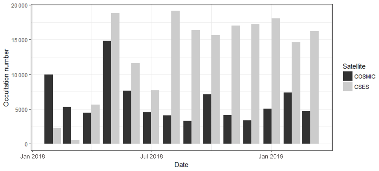
Figure 1 Occultation number per month from February 2018 to March 2019 for both CSES and COSMIC.

From Fig. 1 it can be seen that over 15 000 occultation events can be obtained by CSES each month, or over 500 per day on average, after the initial in-orbit testing stage from February to July 2018. In contrast, occultation numbers from COSMIC are much lower; there are only about 200 occultations on average each day. A total of over 86 000 occultation events have been obtained from the COSMIC data center from February 2018 to March 2019.

Based on these two datasets from CSES and COSMIC, the co-located occultations within defined spatial and temporal criteria from the two measurements are selected and used to carry out the comparison work.

2.2 Data selection

In order to make the comparison between CSES and COSMIC RO data as accurate as possible, spatial and temporal criteria must be defined to select matching occultation profiles for subsequent comparison analysis.

Before determining the selection criteria, it should be pointed out here that RO-retrieved electron density profiles are different from those obtained by vertical ISR observations. For the latter, the observation point is fixed, and all the data points of different altitudes on the profiles correspond to this fixed observation point; but for the former, both the LEO and GPS are in motion during the occultation process, and therefore data points of different altitudes on the profile correspond to different point on the ground. The geographic location of the tangent points of a RO-retrieved profile may vary by several hundred kilometers, which means the spatial range of a profile can cover several degrees in horizontal latitudinal and longitudinal range, and several hundred kilometers in vertical altitude range. However, the ionospheric spatial correlation can extend to a large area, as suggested by some research (Shim et al., 2008; Yue et al., 2007). According to Shim et al. (2008), the daytime meridional correlation lengths are approximately 9 and 5^∘ at middle and low latitudes, and the nighttime values are about 3 and 2^∘ at middle and low latitudes, respectively; the zonal correlation lengths are 23^∘ at midlatitudes and 15^∘ at low latitudes during the day, and are 11^∘ at midlatitudes and 10^∘ at low latitudes during the night. Therefore, the matching profile pairs from the two missions must be within the correlation distances. Considering the relatively small number of occultation events from the COSMIC measurements, we define the search criteria for co-located occultation events as follows: (1) the time difference between the matching occultation pairs is less than 30 min; (2) the distance differences between the locations of the two occultation events are within 2^∘ × 6^∘ range in latitudinal and longitudinal directions. Here, the tangent point at the F2 peak value of an occultation profile is defined as the location of the occultation event. The reason to use the peak value tangent point as the occultation location is because the peak value is normally located at the middle of a profile for the CSES EDPs, and in this way the spatial differences of the corresponding points, especially the top and bottom points, between the matching profile pairs can be limited to the correlation distance range as much as possible.

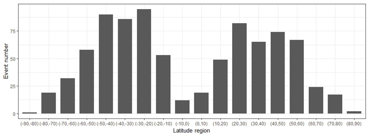
Based on the above criteria, the RO profiles from CSES and COSMIC, covering the period from February 2018 to March 2019, are searched to select the co-located profile pairs. The profiles with NmF2 appearing below 200 or above 500 km are discarded, and profiles with only an ascending or descending part of a profile which cannot determine the peak values are also deleted from the CSES dataset. A total of 845 matched profiles are found, and their distributions are given in Fig. 2. Numbers of occultation in each 10 latitudinal region are also calculated and given in Fig. 3.

Figure 2 Distribution of the selected profile pairs. (Each dot indicates the location of the tangent point of the maximum values in a profile.)

Figure 3 Number of co-located profile pairs along latitudinal regions.

From Fig. 2, it can be seen that the selected profile pairs are globally distributed, which makes the data representative of the whole dataset on a spatial scale. In addition, the time coverage of the co-located occultation pairs is over a year, including different periodic components of the ionospheric variations, which also makes the data involved in the comparison representative on a temporal scale.

It is necessary to note that because the CSES satellite is in a sun-synchronous orbit as mentioned earlier, the local time of the occultation events is concentrated around the ascending (02:00) and descending (14:00) local time, while COSMIC data cover all the local time. Therefore, special attention should be paid to the local-time issue when combing CSES and COSMIC RO data together for data analysis; that is, occultation events with similar local time as that of CSES must be selected from the COSMIC dataset. This local time issue is not considered by Cheng et al. (2018) when they compared CSES RO data with that from COSMIC; therefore their result is questionable.

Another point to note is that most of the selected profile pairs are distributed in the midlatitude regions, as shown in Figs. 2 and 3, and the equatorial region as well as the high-latitude regions exhibit a lower number of occultation events, which ensures that the selection criteria can be satisfied for most of the selected matched profiles.

2.3 Comparison method

The CSES RO electron density data are compared with the co-located COSMIC RO data to assess the consistency and reliability of the CSES RO data relative to the COSMIC data, and then the consistency and reliability of the CSES RO data relative to ground-based measurements are estimated using the results obtained by previous research on COSMIC RO data according to error propagation rules.

The maximum electron density and its height, namely NmF2 and hmF2 from CSES RO data, are compared and analyzed directly with the corresponding co-located COSMIC data, respectively. Besides RO peak values, the profiles of the matched pairs are also compared in this study. To compare the similarities of the profiles, average electron density data near some special altitudes of a profile are calculated and compared. Because the orbit altitude of CSES is 507 km, only data below this altitude are obtained from the CSES RO-retrieved EDPs. Therefore, some altitudes below this altitude are selected, including 100, 150, 200, 250, 300, 350, 400, 450, and 500 km. It should be pointed out here that selection of these altitudes is made for the simplification and ease of calculation. The consistency and reliability of the CSES RO profiles are thus evaluated by combining the comparison results of these selected altitudes.

Normally, the height resolution in the F region is of the order of 20 km for the COSMIC RO (Kuo et al., 2004), but CSES RO data have a higher resolution due to the higher sampling rate of the radio signals. We therefore use the average data between the selected altitudes ±10 km, which are just within the vertical resolution of the COSMIC RO data.

In this study, all the selected matched profiles are involved in the analysis rather than those observed in geomagnetically quiet days. In this way, disturbed data caused by events such as geomagnetic storms can also be used to compare their similarities or differences under these special occasions.

3 Results and discussions

3.1 Comparison of NmF2

The maximum electron density in the ionospheric F2 layer, NmF2, is the most important parameter in ionosphere-related studies. To compare this parameter, the maximum electron density data are extracted from all the matched RO files of CSES and COSMIC measurements. A scatter plot of these matched NmF2 points is given in Fig. 4; also given is the histogram of the data differences between the matched peak value points. As shown in Fig. 4b, data differences between the two measurements are normally distributed; points with data differences exceeding 3 times the RMSE, shown as open circles in Fig. 4a, are considered outliers and can be eliminated from the selected dataset according to the 3σ rule. Red points in Fig. 4a are peak values observed during geomagnetic storm conditions of Dst < −30 nT and all are within 3σ limits and matched very well, as shown in Fig. 4a. Figure 4a also gives the linear fitting equation, the goodness-of-fit coefficient R² (square of correlation coefficient), and the number of data points after the elimination of outliers.

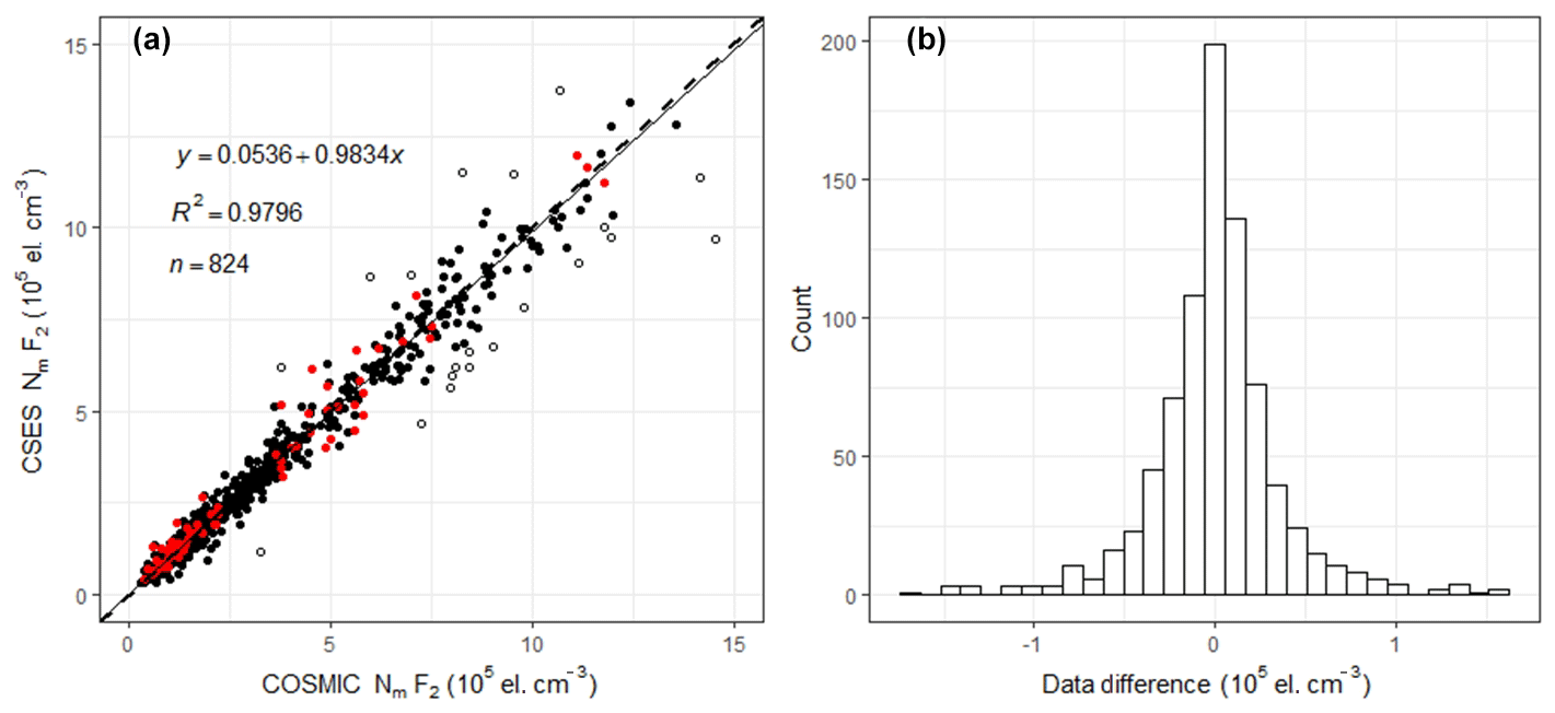
Figure 4 Scatter plot of matched NmF2s and histogram of the data differences between the two sets. The dashed line in (a) is the equal value line with a slope of 1, and the solid line is the linear fitting line. Open circles are points exceeding 3 times the RMSE. Red solid points are data observed when Dst < −30 nT. y refers to CSES NmF2 data, x COSMIC NmF2 data. R² is the goodness-of-fit coefficient; n is the total data number after eliminating outliers.

The correlation coefficient between the two matched NmF2 sets after the elimination of outliers is 0.9898, and the correlation coefficient before the elimination of outliers is 0.9795, both of which can pass the significance test of a 0.01 confidence level. The high correlation coefficient indicates the high consistency between the two NmF2 sets. The linear fitting coefficient of 0.9834 given in Fig. 4a is very close to 1; the data differences between the two sets are nearly normally distributed, as shown in Fig. 4b, and most of the data differences is around zero, all of which mean that the CSES NmF2s are almost equal to COSMIC NmF2s with a nearly-zero bias. Both the correlation coefficient and the linear fitting coefficient indicate that the CSES NmF2s are in extremely good agreement with the corresponding COSMIC data.

To quantify the error, we also calculate the RMSE and relative RMSE between the two sets. The mean of the data differences between CSES NmF2 and COSMIC NmF2 is 0.005363×10⁵ cm⁻³, and the RMSE between the two matched datasets is 0.3638×10⁵ cm⁻³, both of which are very low when compared with the original data. Therefore, the nearly-zero bias between the two measurements of NmF2 can be neglected, which is in accordance with the normal distribution, with most data differences clustering around zero, as shown in Fig. 4b. The mean relative differences or mean relative deviation (MRD) of NmF2 is 1.97 %, and the corresponding relative RMSE is 16.17 %. The MRD is also extremely low. The mean of data differences and the mean of relative data differences, as well as their RMSEs, again show that the CSES RO data are in very good agreement with the COSMIC data.

To compare the difference in the correlation relationship for daytime and nighttime data, the data in Fig. 4 are divided into two groups. As introduced in Sect. 2.2, the time of the CSES satellite is fixed at 02:00 LT during the night and 14:00 LT during the day, and the local times of RO data are around these two fixed local times; we therefore do not need to further consider differences caused by different local times.

The scatter plots for daytime and nighttime data are drawn using the same method introduced above and given in Fig. 5. The data obtained under geomagnetic storm conditions are also shown in red color, all of which are within the 3σ limits.

Figure 5 Scatter plot of NmF2 for daytime and nighttime data. (The dashed line in a and b is the equal value line with a slope of 1.)

The correlation coefficient for daytime data after the elimination of outliers is 0.9759, and 0.9628 before the elimination of outliers; for nighttime data after the elimination of outliers, the correlation coefficient is 0.9249, and 0.8916 for all the data. The higher daytime correlation coefficient indicates a better agreement for the daytime data than the nighttime data. This can be seen clearly from Fig. 5; the nighttime data obviously fluctuate more violently.

The mean data difference for daytime data is $-\mathrm{0.04346}\times {\mathrm{10}}^{\mathrm{5}}$ cm⁻³, with a RMSE of 0.5865×10⁵ cm⁻³, and the mean data difference for nighttime data is 0.01215×10⁵ cm⁻³, with a RMSE of 0.1998×10⁵ cm⁻³. The opposite sign of the daytime and nighttime mean data differences indicates that the CSES daytime data are slightly lower than that of the COSMIC, while CSES nighttime data are slightly higher than the corresponding COSMIC data, but both the means of data differences are extremely low and can be considered to have zero bias when compared with the original measurements.

Table 1 Absolute and relative error of NmF2 between CSES and COSMIC.

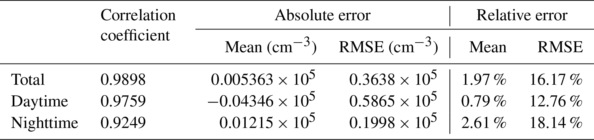
Results of all the coefficients and absolute errors maintain four significant digits, and relative errors maintain two digits after decimal point. Zeros are padded after the decimal point for some results to maintain an identical power exponent.

When comparing the different results given in Table 1, the absolute mean data differences for daytime data are obviously greater than those of the overall result, and with a larger RMSE, and the mean data differences for nighttime data are also greater than the overall result, but with a lower RMSE. It seems that nighttime data are in better agreement than daytime data. However, the two plots in Fig. 5 indicate that the daytime data is obviously better than the nighttime data. This is because the daytime data are much higher than nighttime data, absolute error cannot correctly reflect the real situation when comparing data values with different magnitudes. We therefore calculate the relative errors for both the daytime and nighttime data. The mean relative data difference for daytime data is 0.79 % with a relative RMSE of 12.76 %, and the mean relative data difference for nighttime data is 2.61 % with a relative RMSE of 18.14 %, which indicates an obviously better agreement for the daytime measurements.

It is necessary to point out that most of the daytime data points with higher values are located below the dashed lines as shown in Fig. 5, which means that the COSMIC NmF2s are larger than those of the CSES, so there is a negative bias between the two sets, while for nighttime data, most of the data points with higher values are above the dashed line, indicating higher CSES NmF2 values, thus there is a positive bias between them. This can also explain why there is a higher correlation coefficient and a smaller mean data difference when combining daytime and nighttime data together.

Another issue should be pointed out here. As can be seen from Table 1, the absolute mean difference for daytime data is negative, while the mean relative difference is positive. Further analysis shows that these different signs are caused by some points with much higher CSES NmF2 values.

Here, we compare our results with previous studies and do some analysis.

Lei et al. (2007) obtained a correlation coefficient of 0.85 when comparing COSMIC NmF2 with observations from 31 globally distributed SPIDR (The Space Physics Interactive Data Resource) ionosondes using data observed in July 2006. Chuo et al. (2013) demonstrated that COSMIC-derived NmF2 values are in good agreement with digisonde observations of different seasons; they also reported an agreement about 0.96 using observations from a lower latitude ionosonde in the Southern Hemisphere using a big dataset from May 2006 to April 2008. Chu et al. (2010) found a correlation coefficient of 0.98 when comparing NmF2s between COSMIC and 60 globally distributed ionosondes belonging to SWPC (Space Weather Prediction Center), NOAA, using data from November 2006 to February 2007. Krankowski et al. (2011) obtained a very good correlation coefficient of 0.986 when validating COSMIC RO data in 2008 using measurements from European midlatitude ionosondes. Our result of 0.9898 is quite similar to or even slightly better than those results, when considering the similar solar activity levels. A relatively high correlation coefficient between CSES NmF2 and ionosondes can be deduced since the correlation transitive conditions are satisfied according to Langford et al. (2001). We therefore obtained that CSES RO derived peak values are in very good agreement with COSMIC and ground-based measurements.

For NmF2 relative errors, Krankowski et al. (2011) obtained a mean relative bias of 0.72 % with a standard deviation of 8.42 %, and the slope of the linear fitting line is 0.994 using a manual selected dataset in Europe, which is better than the results in this paper. Wu et al. (2009) got a −3.2 % relative bias with a standard deviation of 20.7 % when comparing NmF2s between COSMIC and 62 global ionosondes from SPIDR using data from July 2006 to December 2007. Yue et al. (2011, 2013) suggest that the ability to retrieve NmF2 using the Abel inversion technique has an uncertainty of about 10 %. Based on the linear fitting equation between CSES and COSMIC and on the NmF2 relative errors between COSMIC and ground-based measurements, we can deduce that the relative errors between CSES peak values and ground-based measurements are comparable to prior results according to error propagation rules.

As to the absolute error, Kelley et al. (2009) obtained a RMSE of 1.0×10⁵ cm⁻³ when comparing COSMIC data with ISR; Hajj and Romans (1998) obtained a NmF2 RMS difference of about 1.5×10⁵ cm⁻³ when comparing the GPS/MET measurements with nearby ionosonde data, and Jakowski et al. (2002) also obtained a similar RMS difference of about 0.9×10⁵ cm⁻³ when comparing the CHAMP RO measurements to the in situ Langmuir probe data on the same satellite. Habarulema et al. (2014) suggested that all RO datasets are close to the ionosonde data within a similar error margin for both midlatitude and low-latitude regions when comparing COSMIC, GRACE, and CHAMP RO data with those of ionosondes. The absolute errors of our results are much smaller than these results, indicating an extremely good agreement between CSES and COSMIC RO NmF2 and further confirming that CSES RO are also within the general error limit as proposed by Habarulema et al. (2014).

The better result of daytime data in this study is in accordance with the conclusion obtained by Wu et al. (2009) and Yue et al. (2011). As we know, the nighttime data have a more complex spatial distribution pattern compared to daytime data, because daytime data are affected by solar radiation, which makes the global distribution pattern of the ionosphere simpler during the daytime. A larger inversion error will be produced when facing an uneven spatial distribution of electron density due to the violence of the spherical symmetry assumption of the Abel inversion method. The complex nighttime spatial distribution can also be proved by the smaller correlation distance during nighttime than that of daytime, as discussed in Sect. 3.2 (Shim et al., 2008).

Besides data obtained on geomagnetically quiet days, data obtained under geomagnetic storm conditions are also quite consistent with each other, demonstrating that the RO data between CSES and COSMIC can remain consistent even under disadvantageous conditions. Hu et al. (2014) suggested that COSMIC measurements are acceptable under geomagnetically disturbed conditions when comparing COSMIC RO data with observations obtained from 2008 to 2013 at Sanya, a lower-latitude ionosonde in China. We therefore deduce that CSES RO data may be acceptable under geomagnetically disturbed conditions, and we will validate this when enough RO data are accumulated.

As suggested by Schreiner et al. (2007), co-located RO soundings allow the precision of the technique to be estimated, but not the accuracy. The results of the nearly-zero bias for both daytime and nighttime data and for the overall data, the normal distribution of the data difference, and the extremely high correlation coefficient between CSES NmF2 and COSMIC NmF2 demonstrate that the CSES NmF2 data are highly consistent and identical with COSMIC measurements, even under geomagnetically disturbed conditions. The consistency and identical nature indicate a similar precision of the two sets. Given the reliability (accuracy) of the COSMIC data proved by many previous studies, we believe that the CSES NmF2 measurements are also quite reliable. Since the co-located data points are globally distributed, the comparison results can be generalized to the overall CSES NmF2 dataset obtained so far.

3.2 Comparison of hmF2

The height of the maximum peak values in the F2 layer, hmF2, is also a very important parameter for ionospheric studies. We therefore also compare this parameter using the corresponding COSMIC dataset.

Comparison of the hmF2 values between the two sets using the same method as that for NmF2, the scatter plot of hmF2, and the histogram of the data differences are given in Fig. 6. Data points exceeding 3 times of RMSE, shown as open circles in Fig. 6a, can be deleted from the selected datasets when calculation is implemented. Again, all the peak height points obtained under geomagnetic disturbed conditions (red points) are within the 3σ limits, as shown in Fig. 6a. It can be seen clearly in Fig. 6a, most of the outliers (open circles) are obviously above the dashed line, which means that occasionally RO data from the CSES dataset will strongly overestimate hmF2 values.

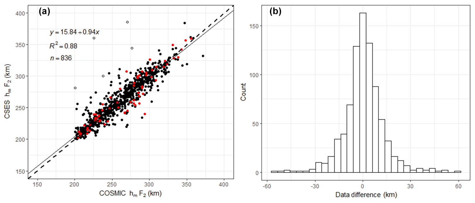
Figure 6 Scatter plot of hmF2s for CSES and COSMIC and histogram of their differences. The dashed line is the equal-value line with a slope of 1, and the solid line is the linear fitting line. The y axis refers to the CSES hmF2, and the x axis to COSMIC hmF2. Open circles are points exceeding 3 times the standard deviation of data differences between matched points. Red points are peak height obtained under geomagnetic conditions of Dst < −30 nT.

The correlation coefficient of hmF2 is 0.9385, slightly lower than that of the NmF2, but can also pass the significance test of confidence level 0.01, which also indicates a very good agreement between the two sets of hmF2. The mean of the hmF2 data differences (CSES hmF2 minus COSMIC hmF2) is 0.59 km, which indicates slightly higher hmF2 for the CSES peak height values, and the RMSE is 12.28 km. hmF2 data difference between the two sets is so small that it can be regarded as nearly-zero bias.

Compared with NmF2, hmF2 data fluctuate more violently. It can be seen from Fig. 6a that some data points obviously deviate from the data cluster, or from the equal-value dashed line. Data points above the dashed line indicate that CSES hmF2s are greater than the corresponding COSMIC data, while data points below the dashed line indicate that the COSMIC hmF2s are greater than that of CSES. Larger errors are produced by these obviously deviating situations. In spite of the data fluctuation, the nearly-zero bias between the two sets, namely the mean data differences, are so small that it can be neglected, which is in accordance with the nearly normal distribution of data differences, as shown in Fig. 6b. The high correlation coefficient and the normally distributed data differences again indicate that the overall hmF2 data of the two sets are in good agreement.

We also compare the daytime and nighttime hmF2s, and the corresponding scatter plots are given in Fig. 7. The correlation coefficient for daytime data is 0.9671 and that for nighttime 0.8510. Similar to NmF2, daytime hmF2 has a better correlation coefficient.

The mean data difference for daytime hmF2s is 0.40 km with a RMSE of 8.59 km, while the mean data difference for nighttime hmF2s is 0.62 km with a RMSE of 14.30 km. The positive means of data differences for both daytime and nighttime data indicate that the overall CSES hmF2s are slightly greater than that of the COSMIC, but they are so small that they can be neglected. The greater RMSE of the nighttime data indicates an obviously more fluctuating nighttime hmF2 compared to the daytime hmF2.

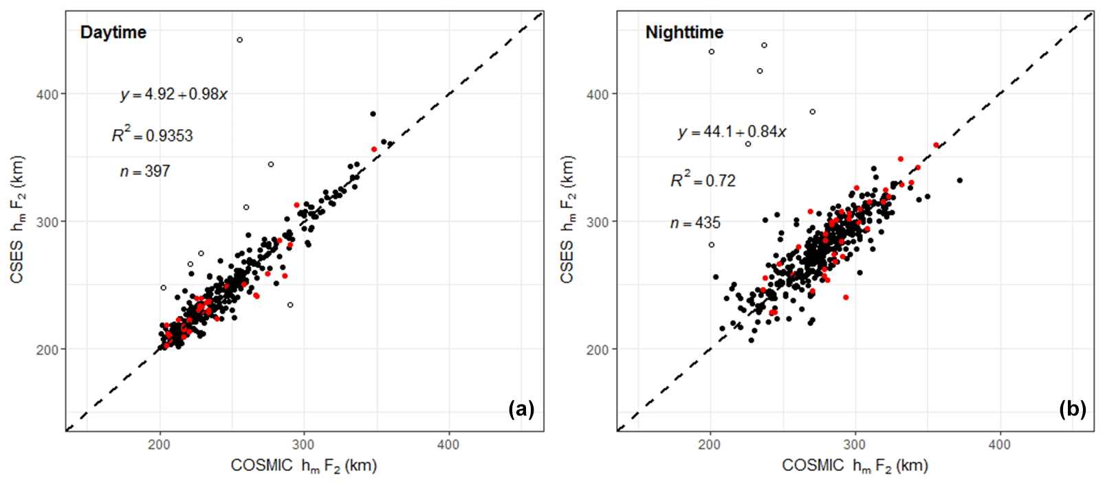
Figure 7 Scatter plot of hmF2 for daytime and nighttime data. The dashed line in Fig. 5 is the equal-value line with a slope of 1.

The bias and RMSE for overall, daytime, and nighttime data are given in Table 2 for a comparison.

Table 2 Absolute error of hmF2 between CSES and COSMIC.

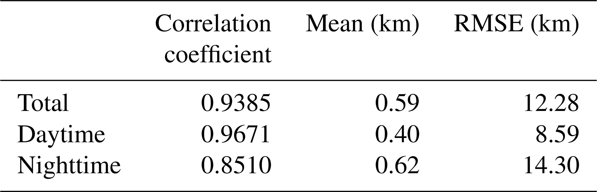
From the results shown in Tables 2 and 1, it can be seen that the correlation of NmF2 is better than that of hmF2 between the two sets. This result is in accordance with the conclusion that the RO measurements were better in NmF2 than in hmF2 (Chuo et al., 2011). Another point is that the daytime hmF2s are in better agreement than the nighttime data, which are similar to NmF2 data.

The overall comparison results of hmF2 are very good when compared to prior COSMIC RO data validation results using ionosonde observations. Chuo et al. (2013) reported an hmF2 agreement of about 0.87 using observations in the low-latitude Southern Hemisphere from May 2006 to April 2008. Krankowski et al. (2011) got a correlation coefficient of 0.949 when comparing COSMIC hmF2 data observed in 2008 with those from ionosondes in European midlatitudes. The high correlation coefficients of our result indicate that the two sets are in good agreement, and the high correlation coefficients between COSMIC hmF2 and ionosondes from previous studies can further prove that CSES hmF2s are consistent with ionosonde observations based on the correlation transitive rule mentioned in Sect. 3.1.

Krankowski et al. (2011) obtained a bias of 2.8 km and a standard deviation of 11.5 km when validating the COSMIC hmF2 data. Cherniak and Zakharenkova (2014) showed that COSMIC hmF2s were in a good agreement with Kharkov ISR observations of different seasons in 2008–2009, and bias and standard deviations are less than 24 and 29 km respectively. Habarulema et al. (2014) obtained an error limit of about 30 km when comparing COSMIC hmF2s with midlatitude ionosondes using data in 2008. Yue et al. (2011) suggested that the retrieval uncertainty in hmF2 is about 10 km for the COSMIC simulation analysis. The nearly-zero bias and the small RMSE between hmF2 of CSES and COSMIC demonstrate that the F region peak height parameters obtained by CSES and COSMIC are extremely similar, or in another way, hmF2s from the two sets have similar precision and accuracy. We therefore deduce that error between CSES hmF2 and ground-based hmF2 is comparable to prior results according to error propagation rules.

As a result, the significant correlation coefficient and very small absolute RMSE in this study indicate the consistent variations and similar precision of hmF2 between CSES and COSMIC, and the nearly-zero bias indicates the two sets have similar accuracy. All of these results indicate that CSES RO-retrieved hmF2s are reliable considering the reliability of COSMIC RO data validated by many previous studies.

3.3 Comparison of electron density profiles (EDPs)

Besides the two most important parameters NmF2 and hmF2, EDPs are also very important because EDPs can provide electron densities at different altitudes to depict ionospheric 3-D images from the bottom of the ionosphere to the altitude of the LEO satellite.

As EDPs from CSES and COSMIC have different altitudes due to the different satellite altitudes of the two missions, only data under the altitude of the CSES satellite can be compared from the co-located profiles. We therefore compare the retrieved EDP data at some selected altitudes as the numbers of data points are not identical for each matched profile pair, and altitudes of retrieved data are not identical for the two co-located profile pairs either.

For each altitude specified in Sect. 2.3, we calculate the average data between ±10 km altitude of each profile and then calculate the correlation coefficients using all the average data pairs at that altitude. The results of all selected altitudes are given in Table 3. Figure 8 gives the scatter plots of all these altitudes, and data obtained under geomagnetically disturbed conditions are shown in red points; also shown in the figure are the linear fitting equations, goodness-of-fit coefficients, and numbers of data points involved in the calculation. Outliers are eliminated from the datasets using the same criteria mentioned above.

Table 3 Correlation coefficients and RMSEs for the data at different altitudes of the profiles.

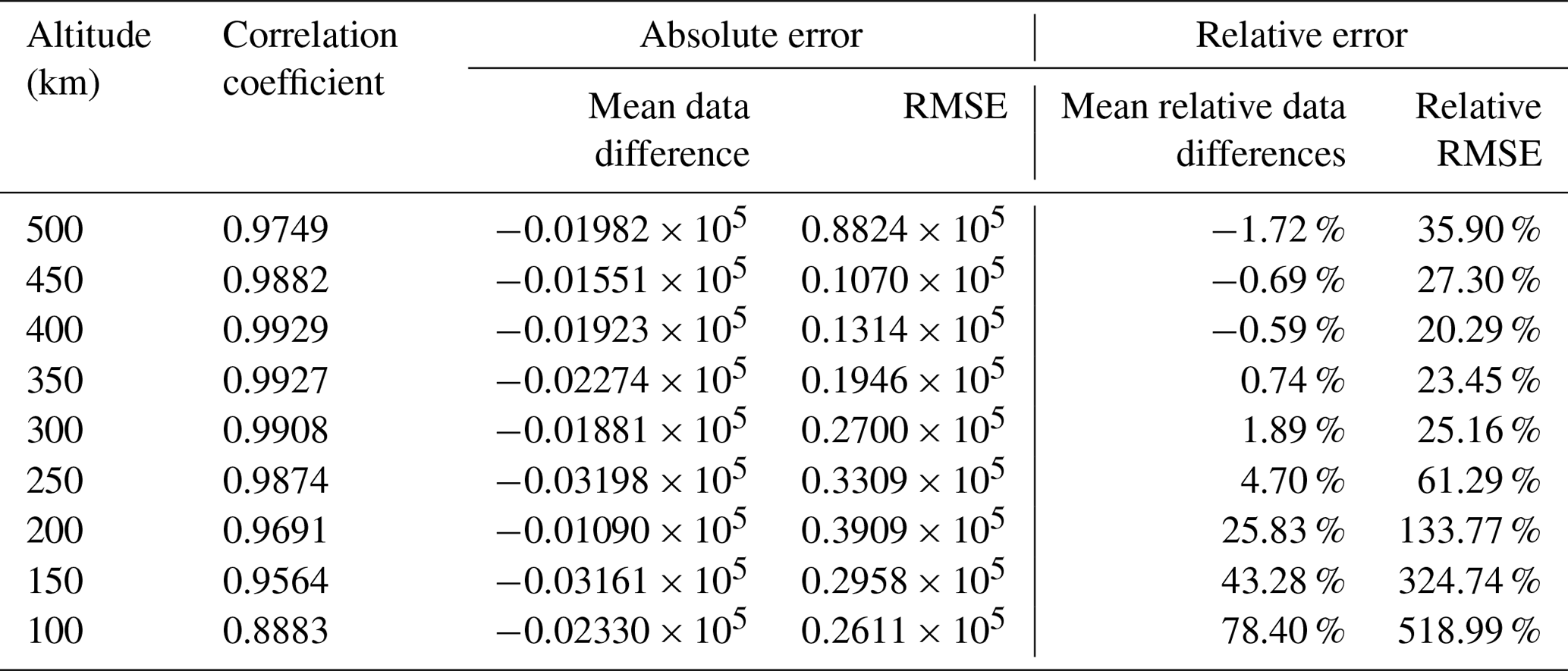
All the correlation coefficients in Table 3 can pass the significance test of confidence level 0.01, which means that data points at different altitudes are highly correlated. When combining all the results together, we can deduce that the co-located profiles from CSES and COSMIC sets are quite similar to each other in spite of the global distribution of these profile pairs, as shown in Fig. 2 in Sect. 2.2. According to some studies, COSMIC profiles are in very good agreement with observations from different ISRs (Lei et al., 2007; Kelley et al., 2009; Cherniak and Zakharenkova, 2014). Pedatella et al. (2015) compared COSMIC RO data at different altitudes with in situ observations from CHAMP and C/NOSF missions and obtained correlation coefficients higher than 0.90, proving the consistency of the COSMIC profiles with in situ satellite observations. Based on the high consistency between CSES and COSMIC profile pairs and previous COSMIC EDP validation results, we can deduce that CSES profiles may generally agree with ISR profiles according to similarity transitive rules mentioned earlier (Langford et al., 2001), which we will further prove by using ISR observations in our subsequent work.

Schreiner et al. (2007) showed that RMS is about 10³ cm⁻³ between 150 and 500 km altitude, whereas below 150 km the RMS increases to a maximum of about 3×10³ cm⁻³ at about 100 km, when comparing the RO profiles from different COSMIC satellites within 5 km distance. Comparing COSMIC profiles with ISR observations, Lei et al. (2007) suggested inversed errors are larger than 10⁵ cm⁻³ at altitudes below ∼150 km, and Cherniak and Zakharenkova (2014) obtained an error range of 12–16×10⁴ cm⁻³. Pedatella et al. (2015) obtained an overall bias of 0.22×10⁵ cm⁻³ with a standard deviation of 0.65×10⁵ cm⁻³, and relative bias and standard deviation are 14.9 % and 10.4 % respectively, when validating COSMIC data at different altitudes using CHAMP in situ observations; they also compared COSMIC data with the in situ observations from the C/NOFS mission and got a relative bias of 5.6 % with a standard deviation 12.4 %. They attributed the better agreement with in situ observations from C/NOFS to the higher altitude of this satellite. Both the absolute and relative errors, as well as error variation with altitude, shown in Table 3, are in accordance with those studies, suggesting that the CSES EDPs are reliable and within general error limits due to the high similarity and consistency between CSES and COSMIC EDPs.

Figure 8 Scatter plots of data from matched profiles at different altitudes. The dashed line in Fig. 5 is the equal-value line with a slope of 1.

From the correlation coefficients given in Table 3, it can be seen that correlation coefficients above 200 km are obviously higher than those below this altitude. The absolute mean differences at different altitudes are comparable to each other. However, relative differences at different altitudes are quite different; relative mean differences above 200 km are extremely small, while relative mean differences below this altitude (including this altitude) increase dramatically. We obtained from Fig. 5 that the peak heights hmF2 of most profiles are located between 200 and 350 km; the obviously high correlation coefficients in these regions indicate that RO-retrieved data at and above peak height are more consistent with each other, whereas discrepancies between the two datasets below the peak regions are much larger. This can be explained by the distribution characteristics of the different ionospheric layers, and by the spherical assumption used in the Abel inversion method. As we know, electron density fluctuations in regions above the F2 peak become smaller under geomagnetically quiet conditions if compared with that at lower altitudes due to the relatively lower density according to electron density attenuation rules; it is therefore easier to satisfy the spherical symmetry assumption when using the Abel inversion method in this region. This spherical symmetry assumption is by far the most significant error source in the retrieval of the electron density profiles (Lei et al., 2007). In addition, a shorter propagating distance in the topside ionosphere for the radio signals from GPS to LEO will lead to a smaller error of straight line propagation assumption. As suggested by Liu et al. (2010), COSMIC RO can obtain reasonably correct electron densities around and above the F2 peak; however, the assumption of spherical symmetry introduces artificial plasma cave and plasma tunnel structures as well as electron density enhancement at the geomagnetic equator at and below 250 km altitude, which will enlarge data discrepancies, as shown in Table 3. Syndergaard et al. (2006) also suggested larger errors at the bottom of the retrieved profiles. The results shown in Table 3 in this study are in accordance with those studies, demonstrating that CSES EDPs have larger errors for data below 200 km altitude, which is similar to that of COSMIC.

An obvious characteristic shown in Table 3 is that all the means of data difference are negative values, though they are very small compared to the original measurements, which means the overall CSES data at different altitudes are lower than the corresponding COSMIC data. The all negative mean data differences at different altitudes may indicate a possible systematic bias between the two measurements. These systematically lower values at all altitudes is most likely caused by the first-order estimation of the electron density at the altitude of the CSES satellite, rather than the spatial differences of the co-located profile pairs, because spatial differences lead to random errors. However, further confirmation of this error source is required. It is also necessary to point out that the signs of the mean relative data differences at altitudes ≥400 km are negative, similar to the signs of the corresponding absolute errors, whereas the signs of the mean relative data differences at altitudes below 400 km are positive, just on the contrary to the signs of absolute mean data differences. Further analysis shows that the opposite signs are caused by points where CSES data are much higher than COSMIC data and thus lead to much larger relative errors, which further indicates that data below the peak regions, especially below about 150 km, fluctuate more violently.

Besides spherical symmetry and straight line propagation assumptions, the larger discrepancies at altitudes below peak regions can be explained by the different spatial locations of the matched profiles. Although the peak values of co-located profile pairs are near each other according to selection criteria, data points other than peak values on the matched profile pairs may exceed the selection criteria and result in larger distances due to the different tangent point path of the matched profile pairs. As a result, a larger distance will lead to larger discrepancies between the corresponding datasets. In addition, the tangent point path of the matched profiles may have different directions, which will lead to different inversion results because the retrieved data represent average electron densities along the radio ray path. In regions with large horizontal gradients, the different ray path can cause obvious differences between the matched profiles. At altitudes below 200 km, especially below 150 km, sporadic E layers can cause large horizontal gradients and then lead to large inversion errors. Wu et al. (2009) suggested that the large relative error below 150 km is due to the errors transferred from upper altitudes (the F layer) and the very small electron density at that altitude. They also suggested that the larger ray separations can induce larger errors which can be transferred to low altitudes; phase measurement errors induce small relative fluctuations in the electron density in the topside ionosphere but can cause large relative fluctuations in the low-altitude ionosphere, because small electron density at low altitude is sensitive to the phase errors. It is therefore concluded that many sources can cause large errors for measurements at altitudes below 150 km, which as a result lead to the large discrepancies between CSES and COSMIC RO data at the bottom of the ionosphere.

Based on the above analysis, we conclude that CSES RO profiles are generally very consistent with those of COSMIC and are reliable for data applications due to the wide acceptance and application of COSMIC RO data. However, larger discrepancies are found at lower altitudes between the two sets compared to data differences at higher altitudes. Therefore, special attention should be paid to data below 200 km in future applications due to the relatively large discrepancies between the two datasets.

4 Summary and conclusions

Validation of the CSES RO data was carried out to estimate the consistency and reliability of the CSES RO data using the globally distributed measurements from the COSMIC mission covering the date range from 12 February 2018 to 31 March 2019, as the consistency and reliability of COSMIC RO data have been widely validated using data from different measurements on a global scale. Comparing CSES NmF2, hmF2, and EDP data at some selected altitudes, with corresponding COSMIC RO data, we obtain the following results.

CSES NmF2 data are highly consistent with that from COSMIC, with a correlation coefficient of 0.9898. The mean data difference is 0.005363×10⁵ cm⁻³ with a RMSE of 0.3638×10⁵ cm⁻³; the relative mean difference is 1.97 % with a relative RMSE of 16.17 %. Correlation between daytime NmF2 data is obviously better than that of nighttime NmF2 data.

CSES hmF2 data are also very consistent with COSMIC data, with a correlation coefficient of 0.9385. The bias between the two sets is 0.59 km with a RMSE of 12.28 km. Again, daytime hmF2 has a better correlation than nighttime data.

Co-located profiles between CSES and COSMIC are generally very consistent with each other, with a better agreement for data at peak height regions (200 km) and above than for those below these regions. For EDP data below 200 km altitude, special attention should be paid due to the relatively larger discrepancies between the two sets.

Based on the validation results between COSMIC data and different measurements obtained by many previous studies and the validation results between COSMIC and CSES RO data obtained in this study, it is deduced that CSES RO data are within the error limits obtained by previous studies according to error propagation rules.

The GOX payload on board CSES satellite can obtain over 500 occultation events each day, which provide a large dataset for the study of the 3-D distribution of the ionospheric electron density when combined with the in situ electron density measurements obtained by the LAP on board CSES. The relatively thorough comparison work in this paper demonstrates that the CSES RO data are very consistent with the corresponding COSMIC data, proving that the CSES RO data are reliable for applications on ionosphere-related problems considering the wide applications of the COSMIC RO data. However, many RO related studies suggest that the asymmetry of the electron density distribution is the main source of the Abel inversion transformation (Schreiner et al., 1999; Syndergaard et al., 2006; Lei et al., 2007), and this inversion error varies with solar activity, season, geomagnetic latitude, and local time (Wu et al., 2009). The CSES RO data in this study cover all the latitudes and four seasons with fixed local times under lower solar activity conditions, and solar activity in this study is similar to that in most of the COSMIC validation studies; the comparison results will therefore applicable to data with similar low solar activity conditions. More subsequent validation work will be conducted and presented using data accumulated under different solar activities.