Characteristics of equatorial plasma bubbles observed by TEC map based on ground-based GNSS receivers over South America

A ground-based network of GNSS receivers has been used to monitor equatorial plasma bubbles (EPBs) by mapping the total electron content (TEC map). The large coverage of the TEC map allowed us to monitor several EPBs simultaneously and get characteristics of the dynamics, extension and longitudinal distributions of the EPBs from the onset time until their disappearance. These characteristics were obtained by using TEC map analysis and the keogram technique. TEC map databases analyzed were for the period between November 2012 and January 2016. The zonal drift velocities of the EPBs showed a clear latitudinal gradient varying from 123 m s⁻¹ at the Equator to 65 m s⁻¹ for 35^∘ S latitude. Consequently, observed EPBs are inclined against the geomagnetic field lines. Both zonal drift velocity and the inclination of the EPBs were compared to the thermospheric neutral wind, which showed good agreement. Moreover, the large two-dimensional coverage of TEC maps allowed us to study periodic EPBs with a wide longitudinal distance. The averaged values observed for the inter-bubble distances also presented a clear latitudinal gradient varying from 920 km at the Equator to 640 km at 30^∘ S. The latitudinal gradient in the inter-bubble distances seems to be related to the difference in the zonal drift velocity of the EPB from the Equator to middle latitudes and to the difference in the westward movement of the terminator. On several occasions, the distances reached more than 2000 km. Inter-bubble distances greater than 1000 km have not been reported in the literature.

Keywords. Ionosphere (equatorial ionosphere; ionospheric irregularities) – meteorology and atmospheric dynamics (thermospheric dynamics)

1 Introduction

Equatorial plasma bubbles (EPBs) are large-scale irregularities that occur in the equatorial ionosphere under particular electro dynamical conditions during the sunset to evening period. The rapid uplift of the evening equatorial F layer due to pre-reversal enhancement of the electric field (PRE) (Rishbeth, 2000) creates a strong density gradient in its bottom side. In this way, irregularities can be triggered in the ionospheric F-layer bottom side, seeding plasma bubbles by the Rayleigh–Taylor instability (Haerendel, 1973; Kelley, 2009). This is believed to be the process by which an EPB is initiated in the F layer. However, EPB seeding process still needs to be well understood (Retterer and Roddy, 2014). Several authors have suggested that perturbations like atmospheric gravity waves (GWs) (Abdu et al., 2009) and large-scale wave structures (LSWSs) (Tsunoda, 2006) could induce F-layer perturbation.

Characteristics of EPBs have been extensively studied using different techniques such as VHF radars (Tsunoda, 1981; Abdu et al., 2009), rockets (Abdu et al., 1991; Muralikrishna et al., 2007), ionosondes (Abdu et al., 1983, 2003, 2012), optical imagers (Pimenta et al., 2003; Arruda et al., 2006; Paulino et al., 2011), GNSS receivers (De Rezende et al., 2007; Takahashi et al., 2014, 2015), and satellites (Huang et al., 2002, 2013; McNamara et al., 2013; Park et al., 2015).

Most of the techniques mentioned above are not able to monitor EPBs continuously in a sufficiently large two-dimensional area. A VHF radar, ionosonde, and all-sky imager can monitor EPBs at a high spatial resolution, making it possible to analyze fine structure of the EPBs. However, they cannot cover a wide range (Abdu et al., 2009; Abdu, 2016). Airglow measurements also depend on favorable weather conditions to produce good-quality optical images (Takahashi et al., 2009). Rocket and satellite observations can also produce ion density profiles in a high spatial resolution; however, its measurements can only be made in situ along the track of each instrument (Muralikrishna et al., 2007; de La Beaujardière et al., 2004). Rocket databases are also limited due to sporadic launching. However, a ground-based network of GNSS receivers is a powerful tool to monitor EPBs by mapping the total electron content (TEC map). The TEC map can cover almost the whole of South America and monitor TEC variability continuously with a time resolution of 10 min. The spatial resolution of the TEC map varies from 50 to 500 km, depending on the density of the observation sites (Takahashi et al., 2016).

In this paper we report the characteristics of the EPBs observed by TEC map based on more than 220 ground-based GNSS receivers over South America. TEC map databases were analyzed between November 2012 and January 2016. A large coverage of the area by the TEC map allowed us to monitor several EPBs simultaneously and get the characteristics of the EPBs from the onset time until their disappearance. We analyzed the following EPB characteristics: (1) latitudinal gradient in both zonal drift velocities of the EPBs and inter-bubble distances, (2) extension and apex height of the EPBs, and (3) inclination of the EPBs against geomagnetic field lines. Among several new observational findings, discussions are focused on the temporal variation of the zonal drift velocities of the EPBs and thermospheric winds, the latitudinal gradient of the plasma drift, and latitudinal dependence of inter-bubble distance.

2 Observations

Ground-based dual-frequency GNSS receiver data have been used to calculate TEC over South America since 2012 by EMBRACE (Brazilian Study and Monitoring of Space Weather). The network GNSS receivers are from the RBMC (Brazilian Network of Continuum Monitoring of GNSS System), RAMSAC (Argentinian Network of Continuum Monitoring of Satellites), IGS (International GNSS Service), and LINS (Low Latitude Ionospheric Sensor Network). All the four networks together provide more than 220 GNSS receivers covering South America.

The GNSS satellites at an altitude of 20 200 km transmit dual-frequency radio signals (f₁=1575.42 MHz and f₂=1227.60 MHz), allowing one to calculate the number of electrons along a tube of 1 m² cross section, between GNSS satellite and the ground receivers, called slant TEC (STEC). In addition, each GNSS satellite transmits pseudo-random noise (PRN), used to identify the source of the signal. Phase and group delays of radio signals are proportional to STEC. A delay of 1 ns corresponds to 2.852 TECU (TEC units), where 1 TECU =10¹⁶ electrons m⁻² column. Each frequency (f₁ and f₂) provides both phase delay (L_1,2) and pseudo-range (P_1,2). STEC can be obtained by calculating L₁−L₂ and P₂−P₁. L₁−L₂ provides only relative changes in STEC. However, P₂−P₁ provides the level of STEC. An absolute STEC is determined using both phase and pseudo-range. Vertical TEC (TEC) is proportional to slant TEC, that is, TEC $=S\times$ STEC, where S is the slant factor. The slant factor is defined as τ₀∕τ₁, where τ₀ is the thickness of the ionosphere (200 km) for the zenith path and τ₁ is the path length of the ray between altitudes of 250 and 450 km. However, the error in TEC increases with increasing slant factor. Therefore, satellite elevation angle less than 30^∘ were discarded in the calculus of TEC (Otsuka et al., 2002).

After TEC calculation, the values are mapped on an ionospheric shell at an altitude of 350 km with a spatial resolution of $\mathrm{0.5}{}^{\circ }\times \mathrm{0.5}{}^{\circ }$ in latitude and longitude. In order to compensate for the lack of data, TEC within a pixel is smoothed temporally with a running average of 10 min and spatially with a running average of 3 × 3 elements covering an area of ∼ 150 km × 150 km. If no data are found in the area, the running average area expands to 5×5 elements (∼ 250 km × 250 km). If the problem persists, the area expands up to 21×21 elements (∼ 1000 km × 1000 km) (Takahashi et al., 2014, 2015). In general, the spatial resolution is 50 to 100 km in the southeastern part of Brazil and 200 to 300 km in the northeastern part (Takahashi et al., 2016). Figure 1 shows a TEC map over South America at 22:50 UT (universal time, 19:50 local time at 45^∘ W) on the night of 24 December 2013. Here, TEC presents a large spatial variations. The red line indicates the geomagnetic equator at 350 km altitude and the dashed white line represents the solar terminator line at 296 km altitude. It can be seen in the TEC map that there is a low-intensity TEC zone along the geomagnetic equator and two crests on both sides of the Equator around ±15^∘ magnetic latitudes. These are due to the equatorial ionization anomaly (EIA). The vertical low TEC belts at approximately 40 and 45^∘ W are most likely signatures of the EPBs.

In this paper, EBPs were defined as (1) a TEC depletion with an amplitude exceeding 10 TECU, (2) a TEC perturbation with at least one well-developed valley, (3) a TEC perturbation with an extension of more than 500 km, and (4) a TEC perturbation lasting more than 1 h.

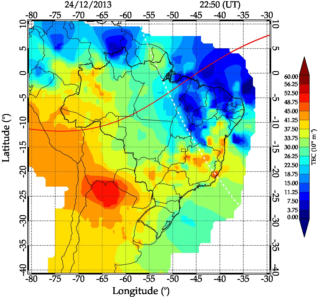
Figure 1 TEC map over South America at 22:50 UT (universal time, 19:50 local time at 45^∘ W) on 24 December 2013. TEC presents a large spatial variations; the color bar varies from 0 to 60 TECU. The red line indicates the geomagnetic equator at 350 km altitude and the dashed white line represents the solar terminator line at 296 km altitude.

2.1 TEC map analysis

Ionospheric plasma bubbles can be observed in the TEC map as a depletion of TEC approximately perpendicular to the geomagnetic equator. From the two-dimensional TEC map, it is possible to calculate the extension and inclination of the EPBs against the geomagnetic field lines. One TEC map at a fixed time is chosen to calculate the length and the inclination. The TEC map that presents a clear development of EPBs and the largest number of EPBs between 01:30 and 02:30 UT was chosen for the analysis. For each EPB a linear fitting over the minimum TEC values is then calculated. The length of the EPBs and the inclination of the EPBs against the geomagnetic field lines are obtained by linear fitting. The inclination of the EPBs is determined as an angle between the linear fitting and the geomagnetic field line. The geomagnetic field line chosen is the line that intercepts the linear fitting at the geomagnetic equator.

2.2 TEC map keogram

Using the TEC maps it is possible to calculate the zonal drift velocities of the EPBs and the inter-bubble distances using the keogram method. A keogram is a collection of west–east slices of TEC maps displayed in a longitude vs. time diagram at a fixed latitude. Figure 2a illustrates a sequence of TEC maps over South America from 20:00 UT on 24 December to 06:00 UT on 25 December 2013. A night of observation corresponds to a total of 61 TEC maps. The horizontal white line at 25^∘ S represents west–east slices of TEC data collected to calculate EPB parameters. Figure 2b shows the result of all west–east slices of TEC data collected from each TEC map arranged side by side as a form of a keogram. The TEC map and the keogram share the same color table. The eastward motion of the EPBs appears as tilted dark-blue lines progressing from west to east throughout the night, indicated by the three dashed black lines (B1, B2, and B3) in the keogram. The dashed and the dot–dash white line represent the nautical and astronomical solar terminator at ∼132 and ∼296 km height, respectively. The zonal drift velocities of the EPBs and the inter-bubble distances were then determined by Δlongitude∕Δt and Δlongitude, respectively, calculated every 10 min for each EPB. The method described above was applied to study eight different latitudes: 0, 5, 10, 15, 20, 25, 30, and 35^∘ S. This methodology allows us to investigate latitudinal gradients in the zonal drift velocities of the EPBs and inter-bubble distances in a large spatial range.

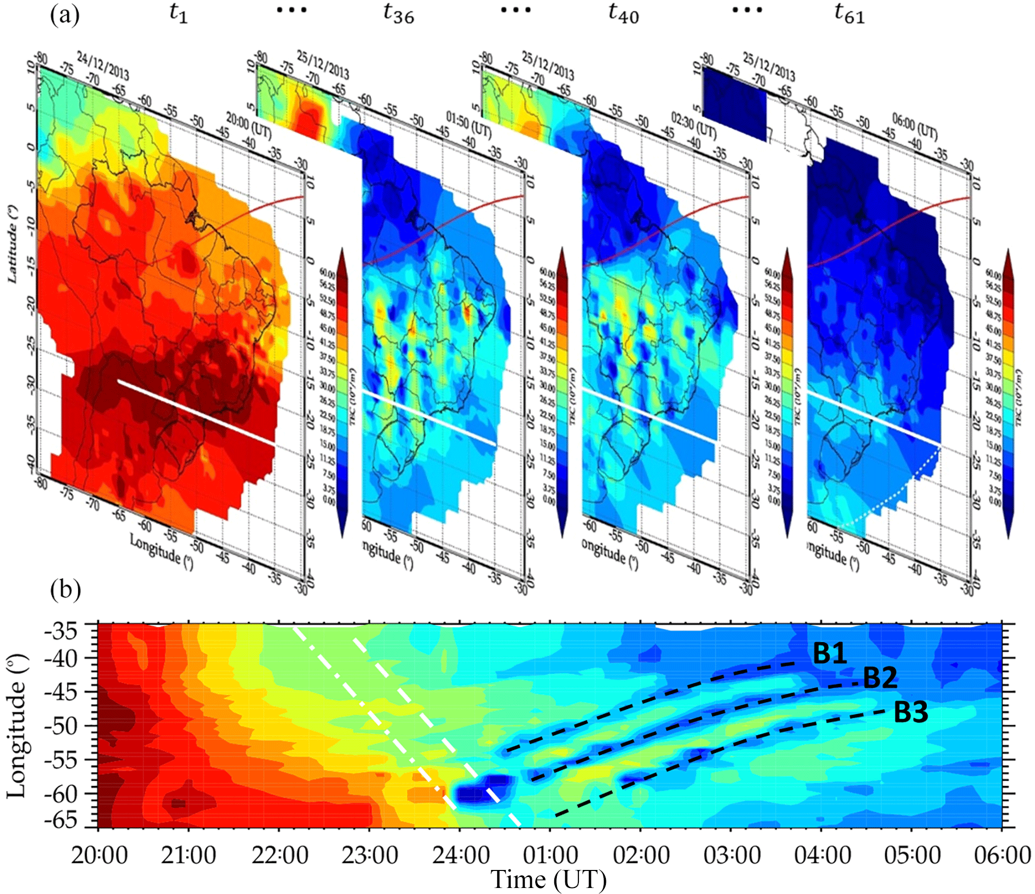
Figure 2 (a) Sequence of TEC maps over South America from 20:00 UT on 24 December to 06:00 UT on 25 December 2013. The horizontal white line at 25^∘ S represents west–east slices of TEC data collected to calculate EPB parameters. (b) Keogram made of all west–east slices of TEC data collected from each TEC map arranged side by side. The black lines indicate the three EPB signatures (B1, B2, and B3) in the keogram. The dashed and the dot–dash white line represent the nautical and astronomical solar terminator at ∼132 and ∼296 km height, respectively.

3 Results

TEC map data were analyzed between November 2012 and January 2016. This corresponds to a high solar activity phase with a solar flux of F$\mathrm{10.7}=\mathrm{127}\times {\mathrm{10}}^{-\mathrm{22}}$ W m⁻² Hz⁻² and included both quiet and magnetically disturbed days.

3.1 Seasonal dependence of occurrence of the EPBs

Figure 3 shows the results for frequency of occurrence of EPBs plotted as percentage for each month of the year. As expected, the largest number of EPBs extends from September to March. The seasonal pattern presented in Fig. 3 shows good agreement with the seasonal variation presented using different techniques for periods of high and low solar activity (Fejer et al., 1999; Abdu et al., 2000; Sahai et al., 2000). The seasonal variation of occurrence of the EPBs is attributed to the seasonal variation of the PRE, which controls the resulting EPB development (Abdu et al., 1981; Tsunoda, 1985; Batista et al., 1996; Sobral et al., 2002). In Fig. 3, no occurrence of EPBs can be seen from May to August due to the EPB criteria discussed in Sect. 2.

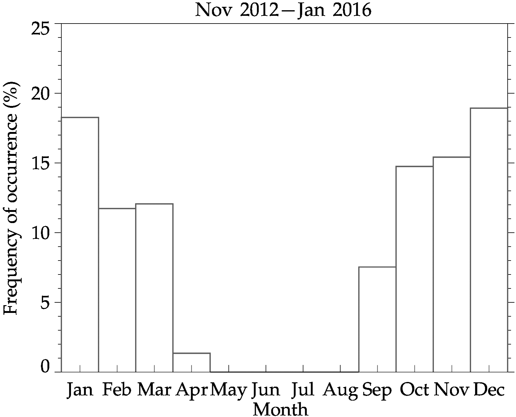
Figure 3 Frequency of occurrence of EPBs plotted as percentage for each month of the year for the period between November 2012 and January 2016.

3.2 Latitudinal extension of the EPBs

Figure 4 shows the seasonal variation of latitudinal extension of the EPBs. The extension is measured by only from the geomagnetic equator to the southern end of the EPBs. Each bar represents an average of all observed extensions for each latitudinal zone. The error bars indicate the standard deviation of the extensions. In January and December the extensions are larger, thereafter starting to decrease and reaching the minimum value in the equinox months. It is known that the extension of the EPBs is related to the apex hight of EPBs (Mendillo and Tyler, 1983; Anderson and Mendillo, 1983; Rohrbaugh et al., 1989; Sahai et al., 1994). However, the apex height depends on the strength of PRE (Haerendel, 1973; Anderson and Haerendel, 1979; Rishbeth, 2000; Kelley, 2009). Therefore, the extension of the EPBs would be longer for the months with large values of PRE.

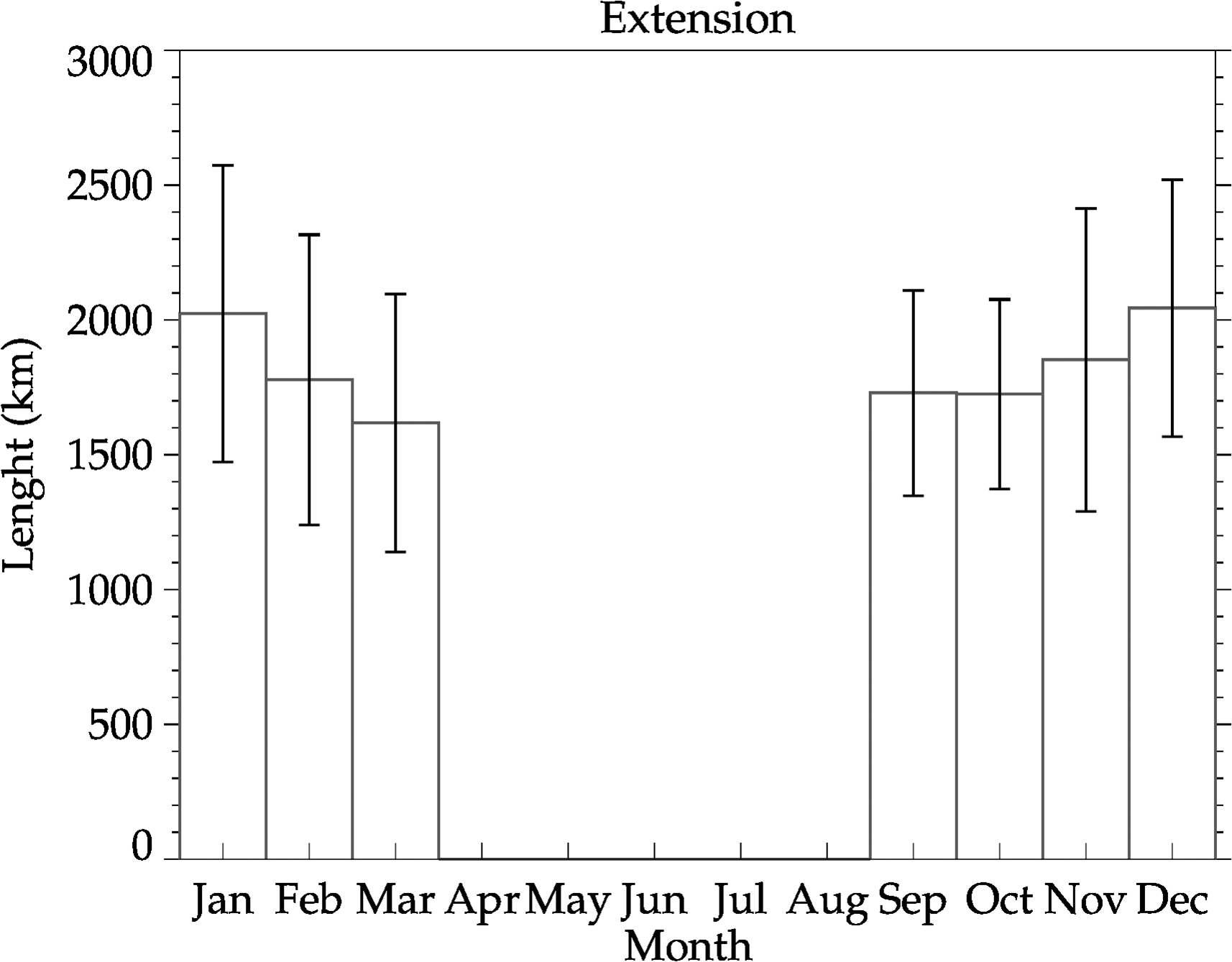
Figure 4 Latitudinal extension of the EPBs over South America measured from the geomagnetic equator for each month of the year.

The development of the EPBs can also be seen as the occurrence of the EPBs for the latitudes of 0, 5, 10, 15, 20, 25, 30, and 35^∘ S as shown in Fig. 5. The apex height is also expressed for each latitude (in blue). The largest number of occurrences of the EBPs displayed in Fig. 5 is between the latitudes 5 and 20^∘ S. The lower occurrence at the Equator is due to low TEC intensity at the geomagnetic equator, which makes the EPB identification difficult. Therefore, it is possible to conclude that 88 % of cases the EPBs can develop up to 20^∘ S, which means the EPBs can rise up to an altitude of 777 km.

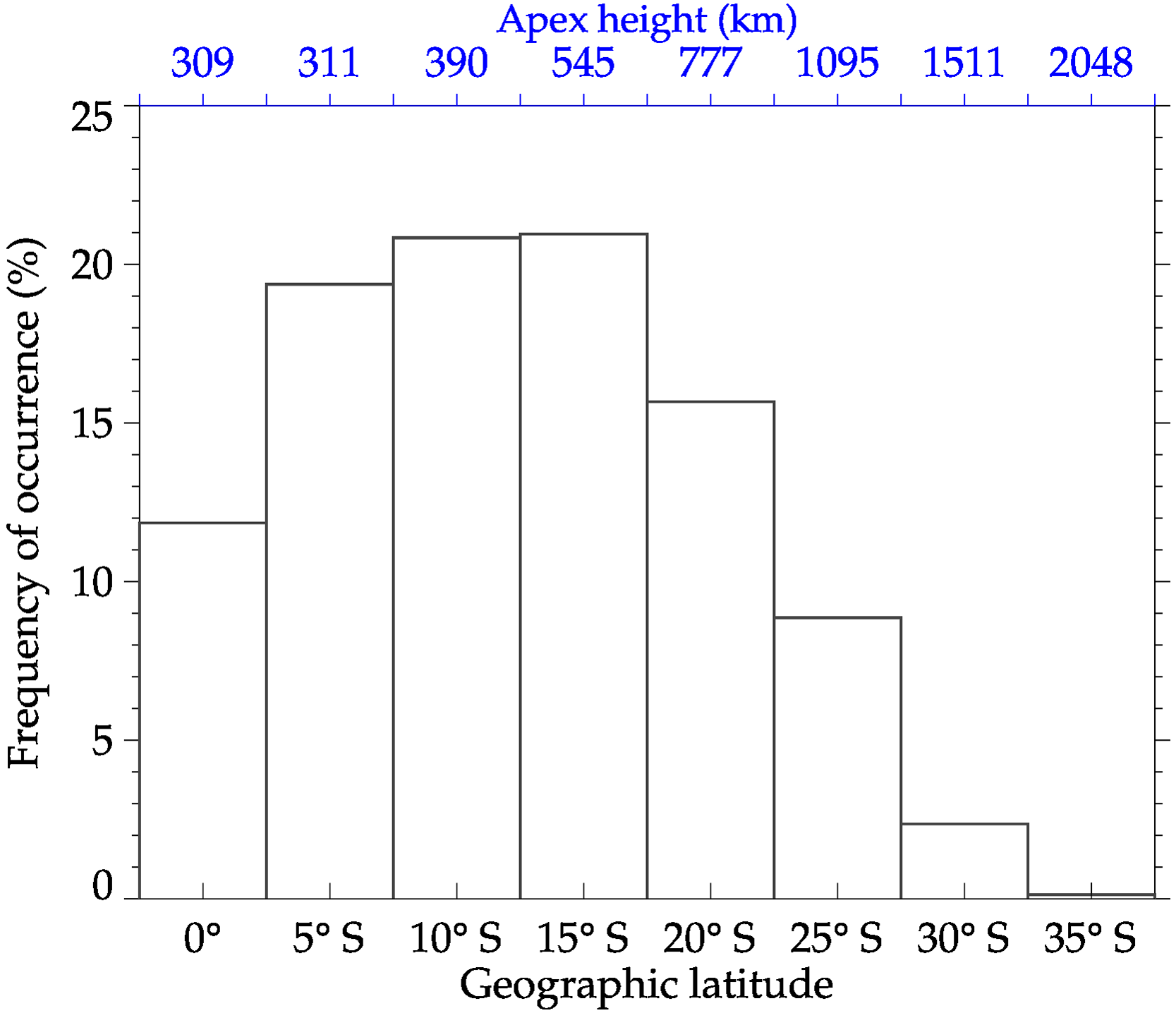
Figure 5 Frequency of occurrence of the EPBs in percentage for the latitudes of 0, 5, 10, 15, 20, 25, 30, and 35^∘ S. Upper horizontal axis (in blue) indicates apex height corresponding to a given geographic latitude.

3.3 Zonal drift velocities of the EPBs

The zonal drift velocities of the EPBs are shown in Fig. 6 for eight different latitudes. Each bar represents an average of all observed velocities for each latitudinal zone. The error bars indicate the standard deviation of the velocities. At the top right corner, the histogram represents all zonal drift velocities of the EPBs at the Equator. The black line represents a Gauss fitting by which the average and the standard deviation was calculated. The zonal velocities present a clear latitudinal gradient varying from 123 m s⁻¹ at the Equator to 65 m s⁻¹ at 35^∘ S latitude. On several occasions, we observed zonal velocities larger than 200 m s⁻¹. The present result, in general, agrees well with the results from previous studies based on data from scanning photometers and imagers (Sobral and Abdu, 1991; Sobral et al., 1999) and an all-sky imager (Pimenta et al., 2003; Martinis et al., 2003), except with the latitudinal gradient, which will be discussed in the next section.

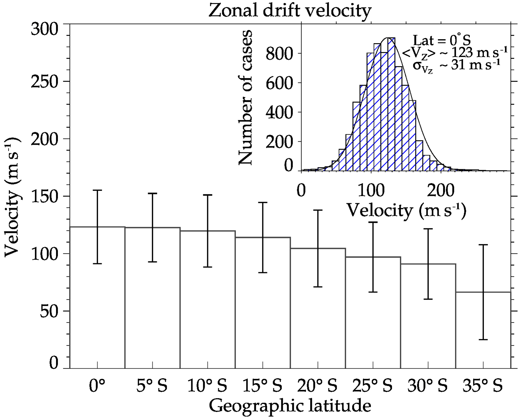
Figure 6 Zonal drift velocities of the EPBs for the latitudes of 0, 5, 10, 15, 20, 25, 30, and 35^∘ S. The histogram (top right corner) represents all observed zonal drift velocities of the EPBs at the Equator.

3.4 Inter-bubble distances

Figure 7 presents the inter-bubble distances with different latitudes. It presents a clear latitudinal gradient varying from 920 km at the Equator to 640 km at 30^∘ S latitude. The error bars indicate how the distances have a large range of variability. On several occasions, we observed distances greater than 2000 km. Values greater than 1000 km have not been reported in the literature yet. Observations of periodic EPBs in South America using airglow emissions of OI 630 nm have found inter-bubble distances of 100 to 500 km (Takahashi et al., 2009; Makela et al., 2010). C/NOFS (Communication/Navigation Outage Forecasting System) satellite measurements found distances reaching 1000 km in post-midnight sector (Huang et al., 2013). These results reinforce the usefulness of TEC maps to study the characteristics of EPBs.

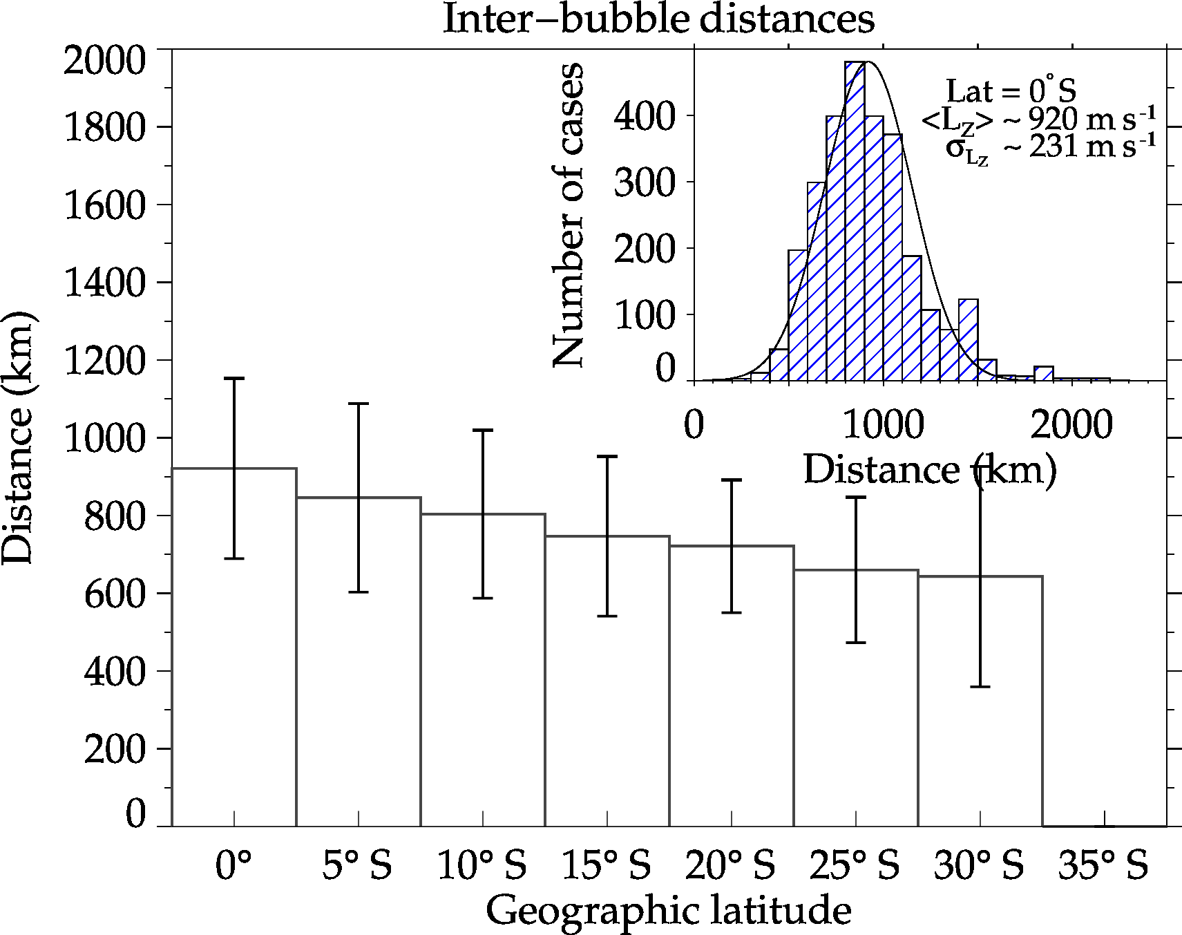
Figure 7 Inter-bubble distances for the latitudes of 0, 5, 10, 15, 20, 25, 30, and 35^∘ S. The error bar indicates standard deviation of all observed distances. The histogram (top right corner) represents all observed inter-bubble distances observed at the Equator.

3.5 Inclination of the EPBs against geomagnetic field lines

Seasonal variation of EPBs inclination against the geomagnetic field lines is shown in Fig. 8. The error bars indicate variability of the inclination during a month. Positives values of inclination mean that the EPBs are tilted to the east of the geomagnetic field lines. In general, inclination of the EPBs is larger in January and December, and then the inclination starts to reverse as it reaches the equinox months. It is known that ionospheric plasma drift and neutral winds are strongly coupled after sunset (Rishbeth, 1981). Therefore, the latitudinal extension of the EPB will be affected by background thermospheric winds. In order to see the neutral wind effect we also plot in Fig. 8 a monthly averaged zonal wind gradient calculated from the Horizontal Wind Model 2014 (HWM14) (Drob et al., 2015) for 350 km altitude, for the period between November 2012 and January 2016. The gradient is obtained from the difference between zonal winds at 0 and 25^∘ S latitude, i.e., dwind = wind(0^∘)–wind(25^∘ S), for a fixed longitude of 55^∘ W, at 02:00 UT. The monthly averaged zonal wind gradient is larger in January, February and December, and then it reverses during the equinox months. The inclination of the EPBs presents a good agreement with the monthly averaged zonal wind gradient calculated from the HWM14. This result suggests that a positive (negative) latitudinal gradient in the zonal wind can make the top (lower) side of a EPB move faster (slower) than the lower (top) side. The differences in the zonal drift velocities could also enhance the angle between the EPBs and geomagnetic field lines.

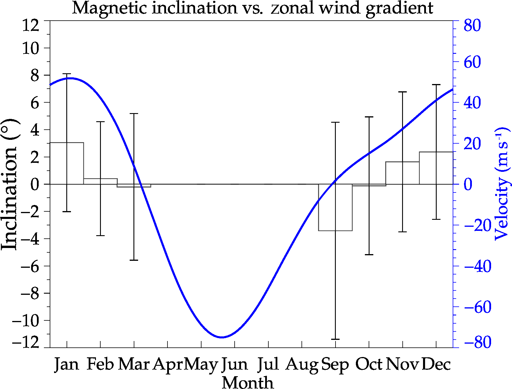
Figure 8 EPB inclination in comparison to the geomagnetic field lines. In blue, monthly averaged zonal wind gradient (dwind) calculated by the Horizontal Wind Model 2014 (HWM14).

4 Discussion

Using a TEC map based on ground-based GNSS receivers, we successfully observed EPBs over South America. The large coverage of the TEC map allowed us to monitor several EPBs simultaneously and obtain characteristics like the EPB velocity, extension, and longitudinal distributions. In addition, in this work we were able to track EPBs from the onset time until their disappearance. Among several new observational findings, three of them should be emphasized: (1) the temporal variation of the zonal drift velocities of the EPBs and thermospheric winds, (2) the latitudinal gradient of plasma drift, and (3) latitudinal dependence of inter-bubble distances.

4.1 Temporal variation of the zonal drift velocities of the EPBs and thermospheric winds

Ionospheric plasma drift is driven by vertical electric fields generated by E- and F-region dynamos (Haerendel et al., 1992). After sunset, the E-region electron density suffers a strong loss (Heelis et al., 1974) and the dynamics of the ionosphere are controlled by the F-region dynamo, which is generated by thermospheric neutral winds. Figure 9 shows the monthly averaged zonal drift velocities of the EPBs at 5^∘ S and the monthly averaged thermospheric zonal wind measured by a OI 630 nm FPI near the Equator during the months when we observed a large occurrence of EPBs. The FPI is able to measure thermospheric zonal and meridional neutral winds by measuring Doppler shift of OI 630 nm emission line at 250 km altitude with an accuracy of 5 to 10 m s⁻¹ (Makela et al., 2011; Meriwether et al., 2011). The FPI is located at São João do Cariri (7.4^∘ S, 36.5^∘ W), Brazil, and the data were obtained between 2013 and 2014. A positive value of thermospheric zonal wind velocity indicates eastward wind, and the error bar indicates deviation estimated by using the Monte Carlo method (Makela et al., 2011). The comparison between the zonal drift velocities of the EPBs and thermospheric zonal wind shows a similar pattern. However, the magnitude of the zonal drift velocities of the EPBs is larger than thermospheric zonal wind velocity. This should be due to the fact that zonal drift velocities of the EPBs observed by TEC is around 350 km altitude, while the OI 630 nm emission peak altitude is approximately at 250 km. Therefore, the difference in zonal velocity between EPBs and thermospheric zonal wind could be attributed to the vertical gradient in the zonal neutral wind. Drob et al. (2015) have modeled vertical profiles of a zonal wind as a function of local time for equinox conditions at São João do Cariri. They found a zonal wind velocity of ∼80 m s⁻¹ at 250 km altitude and ∼120 m s⁻¹ at 350 km altitude at 24:00 UT, and thereafter the vertical gradient starts to decrease along the night. The results presented in Fig. 9 show a good agreement with the vertical gradient in the zonal neutral winds modeled by Drob et al. (2015).

Figure 9 Monthly averaged of the zonal drift velocities of the EPBs (in red) and the thermospheric zonal wind measured by a OI 630 nm FPI (in blue) during the months of large occurrence of the EPBs (October to March).

4.2 Latitudinal gradient of plasma drift

The zonal drift velocities of the EPBs present a clear latitudinal gradient varying from 123 m s⁻¹ at the Equator to 65 m s⁻¹ at 35^∘ S as presented in Fig. 6. This latitudinal gradient in the zonal drift of the EPBs has been attributed by several authors to a latitudinal gradient in the zonal neutral wind velocities (Sobral and Abdu, 1991; Martinis et al., 2003). Pimenta et al. (2003) reported a significant latitudinal variations in the zonal drift velocities of the EPBs observing it from two different latitudinal zone, one at São João do Cariri (7.4^∘ S) and the other at Cachoeira Paulista (22.7^∘ S), Brazil. They observed a region of low zonal drift velocity located near 10^∘ S and attributed it to the increase in the electron density in the EIA region. From the present result, however, we could not see such latitudinal variability; instead, we observed zonal drift velocities of the EPBs decreasing monotonically with latitude as seen in Fig. 6. The two different pieces of observational evidence caught our attention. One possibility to explain could be that the two observations have been carried out in the different solar cycle conditions, which means a different intensity of EIA. According to Huang and Cheng (1996), the strength of the EIA crest increases with the increasing of solar flux. It should be noted that, for the period between November 2012 and January 2016, the solar flux was F$\mathrm{10.7}=\mathrm{127}\times {\mathrm{10}}^{-\mathrm{22}}$ W m⁻² Hz⁻² compared F$\mathrm{10.7}=\mathrm{171}\times {\mathrm{10}}^{-\mathrm{22}}$ W m⁻² Hz⁻² for the period between December 1999 and February 2000 analyzed by Pimenta et al. (2003). This means that the solar flux of our present observation period was more than 25 % lower than the period analyzed by Pimenta et al. (2003). In order to confirm the effect, however, further investigation using dynamical ionospheric model simulations would be necessary.

4.3 Latitudinal dependence of inter-bubble distances

In Fig. 7 we showed that the inter-bubble distances reduce from the Equator to middle latitudes. There might be two factors to be considered in the reduction of distance. One is the difference in the zonal drift velocities of the EPBs due to different thermospheric zonal wind velocity from the Equator to middle latitudes and the other is the difference in the westward movement of the terminator (Huang et al., 2013). If one assumes that EPB seeding and development happen near the solar terminator passage and a successive EPB occurs soon after as the result of a periodic perturbation of the F-layer bottom side and the passage of the terminator (Tsunoda, 2006; Abdu et al., 2009; Takahashi et al., 2009; Makela et al., 2010). The distance between successive EPBs will, therefore, be determined by the velocity of the EPB and the terminator movement. For example, at the Equator, the zonal drift velocities of the EPBs were 123 m s⁻¹ (Fig. 6) and the rotation speed of the Earth is 465 m s⁻¹. In this case, the EPB will be 920 km away from the terminator after ∼1570 s. However, in the middle latitudes, the zonal drift zonal velocities of the EPBs and the terminator movement away from each other will be slower. Consequently, the inter-bubble distances will be smaller. For example, at 35^∘ S, the zonal drift velocities of the EPBs was ∼65 m s⁻¹ (Fig. 6) and the rotation speed of the Earth is 380 m s⁻¹, which means that the EPB should be 700 km away from the solar terminator after ∼1570 s.

5 Conclusions

We reported the characteristics of EPBs observed by TEC map based on more than 220 ground-based GNSS receivers over South America. These characteristics were obtained by using TEC map analysis and keograms. TEC map databases analyzed were for the period between November 2012 and January 2016. The observational period corresponds to a high solar activity phase with a solar flux of F$\mathrm{10.7}=\mathrm{127}\times {\mathrm{10}}^{-\mathrm{22}}$ W m⁻² Hz⁻² and includes both quiet and magnetically disturbed days. Our main conclusions are as follows:

1. EPBs occurred mainly from September to March. The latitudinal extension of the EPBs is larger for the months of January and December, and the extension start to decrease as it reaches the equinox months, which seems to agree with the seasonal variation of PRE. In 88 % of the cases the EPBs developed up to 20^∘ S, indicating that the apex height was of 777 km altitude.

2. EPB zonal drift velocities presented a clear latitudinal gradient varying from 123 m s⁻¹ at the Equator to 65 m s⁻¹ at 35^∘ S. The comparison between zonal drift velocities of the EPBs and the thermospheric zonal winds observed by FPI presented the same pattern; however, the magnitude of zonal drift velocities of the EPBs was larger than thermospheric zonal wind velocity. This might be attributed to a vertical gradient in the zonal wind.

3. The inter-bubble distances also showed a clear latitudinal gradient varying from 920 km at the Equator to 640 km at 30^∘ S. The latitudinal gradient in the inter-bubble distance seems to be related to the difference in the zonal drift velocities of the EPBs from the Equator to middle latitudes and also to the difference in the westward movement of the terminator. On several occasions, the distances reached more than 2000 km at the Equator.

4. The latitudinal extension of EPBs occasionally presents a significant inclination against the geomagnetic field lines. The inclination of the EPBs is larger in January and December, and the inclination starts to reverse as it reaches the equinox months. The inclination of the EPBs shows a good agreement with the monthly averages zonal wind gradient calculated by HWM14.