Non-Gaussianity and cross-scale coupling in interplanetary magnetic field turbulence during a rope–rope magnetic reconnection event

In a recent paper (Chian et al., 2016) it was shown that magnetic reconnection at the interface region between two magnetic flux ropes is responsible for the genesis of interplanetary intermittent turbulence. The normalized third-order moment (skewness) and the normalized fourth-order moment (kurtosis) display a quadratic relation with a parabolic shape that is commonly observed in observational data from turbulence in fluids and plasmas, and is linked to non-Gaussian fluctuations due to coherent structures. In this paper we perform a detailed study of the relation between the skewness and the kurtosis of the modulus of the magnetic field $\left|\mathit{B}\right|$ during a triple interplanetary magnetic flux rope event. In addition, we investigate the skewness–kurtosis relation of two-point differences of $\left|\mathit{B}\right|$ for the same event. The parabolic relation displays scale dependence and is found to be enhanced during magnetic reconnection, rendering support for the generation of non-Gaussian coherent structures via rope–rope magnetic reconnection. Our results also indicate that a direct coupling between the scales of magnetic flux ropes and the scales within the inertial subrange occurs in the solar wind.

Keywords. Space plasma physics (turbulence)

1 Introduction

The solar wind can be regarded as a network of entangled magnetic flux tubes and Alfvénic fluctuations propagating within each flux tube (Bruno et al., 2001; Borovsky, 2008). Flux tubes can emerge locally in the solar wind as a consequence of the magnetohydrodynamic turbulent cascade (Matthaeus and Montgomery, 1980; Veltri, 1999; Greco et al., 2008, 2009; Telloni et al., 2016). An alternative view describes coherent structures as “fossile” structures that emanate from the solar surface and are advected by the solar wind (Borovsky, 2008; Bruno et al., 2001).

The probability distribution functions (PDFs) of turbulent space plasmas display sharp peaks and fat tails on small scales within the inertial subrange (Sorriso-Valvo et al., 2001; Bruno et al., 2001; Koga et al., 2007; Chian and Miranda, 2009), as well as departures from self-similarity and monofractality (Bershadskii and Sreenivasan, 2004; Bruno et al., 2007; Miranda et al., 2013). These features are due to the presence of rare, large-amplitude coherent structures which dominate the statistics of fluctuations on small scales and can be quantified by the computation of statistical moments.

A robust parabolic dependence between the normalized third-order moment (skewness) and the normalized fourth-order moment (kurtosis) has been found in local concentrations of contaminants in atmospheric turbulence as found by Mole and Clarke (1995). Sura and Sardeshmukh (2007) also found a similar skewness–kurtosis parabolic relation using global data of sea-surface temperature fluctuations. Labit et al. (2007) reported a similar skewness–kurtosis dependence in electron density fluctuations in plasma confinement experiments. Medina and Díaz (2016) obtained a skewness–kurtosis parabolic relation for datasets of human reaction times for visual stimuli. Since then, the presence of a skewness–kurtosis relation in different physical scenarios has attracted much attention (Krommes, 2008; Sattin et al., 2009; Sandberg et al., 2009; Guszejnov et al., 2013; Bergsaker et al., 2015) and has been associated with the presence of non-Gaussian fluctuations due to coherent structures (Labit et al., 2007; Sandberg et al., 2009; Guszejnov et al., 2013; Bergsaker et al., 2015). The skewness–kurtosis parabolic relation was also found in time series of two-point differences of the modulus of the magnetic field by Vörös et al. (2006). They demonstrated that the parabolic relation is due to nonlocal interaction between large-scale structures and small-scale intermittency.

In this paper we investigate the skewness–kurtosis relation during a triple interplanetary magnetic flux rope (IMFR) event detected by Cluster-1 in the solar wind. This event was recently characterized by Chian et al. (2016). They demonstrated the occurrence of magnetic reconnection at the interface region of two IMFRs and that this reconnection can be the origin of interplanetary intermittent turbulence. Our results show that the skewness–kurtosis parabolic relation is enhanced during the reconnection between flux ropes, and that is a natural consequence of the interaction between flux ropes.

This paper is organized as follows. Section 2 presents the statistical tools employed for the data analysis, including the equations to compute the skewness and the kurtosis. Section 3 describes the triple-IMFR event. The skewness–kurtosis relation is analyzed in detail in Sect. 4. The interpretations of these results are presented in Sect. 5. Finally, we conclude in Sect. 6.

2 Data analysis tools

Let θ_i, $i=\mathrm{1},\mathrm{\dots },N$ be the time series of a quantity of interest (e.g., the modulus of the magnetic field $\left|\mathit{B}\right|$). The skewness of θ_i can be computed as follows:

$$\begin{array}{}\text{(1)}& {\displaystyle }{\displaystyle }S={\displaystyle \frac{\mathrm{1}}{N}}\sum _{i=\mathrm{1}}^N{\left({\displaystyle \frac{{\mathit{\theta }}_i-〈{\mathit{\theta }}_i〉}{\mathit{\sigma }}}\right)}^{\mathrm{3}},\end{array}$$

where 〈θ_i〉 represents the average of θ_i, N represents the number of data points, and σ is the SD of θ_i. The flatness of θ_i is given by

$$\begin{array}{}\text{(2)}& {\displaystyle }{\displaystyle }F={\displaystyle \frac{\mathrm{1}}{N}}\sum _{i=\mathrm{1}}^N{\left({\displaystyle \frac{{\mathit{\theta }}_i-〈{\mathit{\theta }}_i〉}{\mathit{\sigma }}}\right)}^{\mathrm{4}},\end{array}$$

from which the kurtosis can be obtained by

$$\begin{array}{}\text{(3)}& {\displaystyle }{\displaystyle }K=F-\mathrm{3}.\end{array}$$

For a Gaussian function $S=K=\mathrm{0}$. The skewness quantifies the degree of asymmetry of the PDF of θ_i, whereas the kurtosis quantifies the departure of the flatness of the PDF of θ_i from the flatness of a Gaussian distribution which is equal to 3. The definition of kurtosis in Eq. (3) is sometimes called “excess kurtosis” (Sattin et al., 2009).

A common way to characterize asymmetry and non-Gaussianity of θ_i as a function of scale τ is through the time series of two-point differences:

$${\displaystyle }\mathit{\delta }{\mathit{\theta }}_i\left(\mathit{\tau }\right)={\mathit{\theta }}_{i+\mathit{\tau }}-{\mathit{\theta }}_i.$$

The skewness of θ_i on scale τ is then

$$\begin{array}{}\text{(4)}& {\displaystyle }{\displaystyle }S\left(\mathit{\tau }\right)={\displaystyle \frac{\mathrm{1}}{N}}\sum _{i=\mathrm{1}}^N{\left({\displaystyle \frac{\mathit{\delta }{\mathit{\theta }}_i-〈\mathit{\delta }{\mathit{\theta }}_i〉}{{\mathit{\sigma }}_{\mathit{\tau }}}}\right)}^{\mathrm{3}},\end{array}$$

and the flatness is

$$\begin{array}{}\text{(5)}& {\displaystyle }{\displaystyle }F\left(\mathit{\tau }\right)={\displaystyle \frac{\mathrm{1}}{N}}\sum _{i=\mathrm{1}}^N{\left({\displaystyle \frac{\mathit{\delta }{\mathit{\theta }}_i-〈\mathit{\delta }{\mathit{\theta }}_i〉}{{\mathit{\sigma }}_{\mathit{\tau }}}}\right)}^{\mathrm{4}},\end{array}$$

where σ_τ is the SD of δθ_i(τ). From Eq. (5) the kurtosis as a function of scale is obtained by

$$\begin{array}{}\text{(6)}& {\displaystyle }{\displaystyle }K\left(\mathit{\tau }\right)=F\left(\mathit{\tau }\right)-\mathrm{3}.\end{array}$$

A functional relation between the skewness and the kurtosis of θ_i as defined by Eqs. (1)–(3) has been observed in a variety of scenarios (e.g., Mole and Clarke, 1995; Labit et al., 2007; Medina and Díaz, 2016). This relation is given by

$$\begin{array}{}\text{(7)}& {\displaystyle }{\displaystyle }K=\mathit{\alpha }{S}^{\mathrm{2}}+\mathit{\beta },\end{array}$$

where α and β are the coefficients that characterize a parabolic curve.

We compute the α and β coefficients by applying a least-square fit between (S,K) values obtained from the observational data and Eq. (7) following the Levenberg–Marquardt algorithm (Levenberg, 1944; Marquardt, 1963; Bard, 1974), which is a popular method to fit a dataset into nonlinear equations. In order to quantify how well the computed (S,K) values are fitted into Eq. (7) we employ the correlation index r which measures the correlation between two datasets X_i and Y_i, $i=\mathrm{1},\mathrm{\dots },N$:

$$\begin{array}{}\text{(8)}& {\displaystyle }{\displaystyle }r={\displaystyle \frac{\mathrm{1}}{{\mathit{\sigma }}_X{\mathit{\sigma }}_Y}}\sum _{i=\mathrm{1}}^N{\displaystyle \frac{(X_i-〈X_i〉)(Y_i-〈Y_i〉)}{N}},\end{array}$$

where σ_X and σ_Y represent the SD of X_i and Y_i, respectively. The correlation index $r\in [-\mathrm{1},\mathrm{1}]$. If r=1 there is complete correlation between X_i and Y_i, whereas $r=-\mathrm{1}$ indicates anticorrelation. The value r=0 represents absence of correlation.

In summary, the analysis is described by the following steps:

• Compute S and K from the modulus of magnetic field $\left|\mathit{B}\right|$ using Eqs. (1)–(3).

• Apply the Levenberg–Marquardt algorithm to find α and β in Eq. (7) that best fit the (S,K) values.

• Use α and β obtained from the previous step in Eq. (7) to obtain empirical values of K as a function of S.

• Compute the correlation index r between the values of K from the previous step and the values of K from the observational data. The r index will measure how close the K values computed by Eq. (3) are to the K values obtained empirically from Eq. (7).

We repeat these steps for S(τ) and K(τ) of two-point differences using Eqs. (4) and (6) in the first step. There are several computational programs for data analysis that implement the Levenberg–Marquardt algorithm. Here we use the implementation available in the GNU Octave program (Eaton, 2012; Eaton et al., 2014).

We note that several papers regarding the relation between skewness and kurtosis have employed the definition of what we refer to as flatness (Eq. 2). Throughout this paper we will focus on the kurtosis defined by Eq. (3).

3 A triple-IMFR event

Figure 1a shows the time series of the modulus of magnetic field $\left|\mathit{B}\right|$ obtained by the FGM instrument onboard Cluster-1 (Balogh et al., 2001) from 00:00 to 12:00 UT on 2 February 2002. During this interval Cluster-1 was in the solar wind upstream of the Earth's bow shock (Chian and Miranda, 2009). The magnetic field data are collected by Cluster-1 at a resolution of 22 Hz (Balogh et al., 2001). Figure 1 also presents an overview of other in situ plasma parameters for the selected interval, namely, the three components of B in the GSE coordinates, the angles Φ_B and Θ_B of the solar wind magnetic field B relative to the Sun–Earth x axis in the ecliptic plane, and out of the ecliptic, respectively, in the polar GSE coordinates; the modulus of the ion bulk flow velocity $\left|{\mathbf{V}}_{\mathrm{i}}\right|$, the ion number density n_i, the ion temperature perpendicular to the magnetic field T_i and the ion plasma β_i, which is the ratio between plasma kinetic pressure and magnetic pressure. The Cluster-1 plasma measurements are given by the ion spectrometry experiment CIS (Rème et al., 2001).

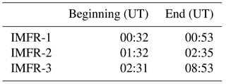
This event is characterized by the presence of three interplanetary magnetic flux ropes. Magnetic flux ropes are magnetic structures described as bundles of twisted, current-carrying magnetic field lines bent into a tube-like shape, spiralling around a common axis (Russell and Elphic, 1979; Telloni et al., 2016; Chian et al., 2016). During this event three IMFRs were identified by Chian et al. (2016) using a combination of criteria for large-scale magnetic cloud boundary layers (Lepping et al., 1997; Wei et al., 2003) and small-scale IMFRs (Moldwin et al., 2000; Feng et al., 2007). The interval of each IMFR is indicated by horizontal arrows in Fig. 1a, and their timings are shown in Table 1.

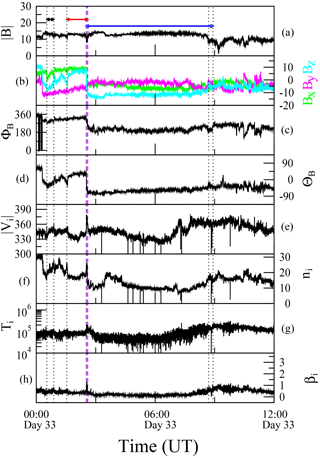
Figure 1 Cluster-1 magnetic field and plasma parameters from 00:00 to 12:00 UT on 2 February 2002. From top to bottom: modulus of magnetic field $\left|\mathit{B}\right|$ (nT), three components of B (nT) in the GSE coordinates, azimuth angle Φ_B (^∘), latitude angle Θ (^∘), modulus of ion bulk velocity $\left|{\mathbf{V}}_{\mathrm{i}}\right|$ (km s⁻¹), ion number density n_i (cm⁻³), ion temperature T_i (eV) and ion plasma beta β_i. Horizontal arrows indicate the interval of IMFR-1 (black), IMFR-2 (red) and IMFR-3 (blue). The front and rear boundary layers of each IMFR are indicated by the vertical dotted lines.

Table 1 Beginning and end of the intervals depicted in Fig. 1, corresponding to the boundary layers of three interplanetary magnetic flux ropes (IMFRs) on 2 February 2002.

4 Skewness–kurtosis relation

4.1 Time series of $\left|\mathit{B}\right|$

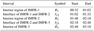
Figure 2a shows the time series of $\left|\mathit{B}\right|$ detected by Cluster-1 on 2 February 2002 (Julian day 32) from 00:32 to 03:18 UT. Five regions were defined during this interval and are indicated using arrows. These regions represent the interior region of IMFR-1 (R₁), the interface of IMFR-1 and IMFR-2 (I₁₂), the interior of IMFR-2 (R₂), the interface of IMFR-2 and IMFR-3 (I₂₃), and the interior of IMFR-3 (R₃). Their timings are indicated in Table 2. Each region has a duration of 30 min, which gives 40 358 data points. During this event current sheets were detected at the front boundary layer of IMFR-1 and at the interface region between IMFR-2 and IMFR-3. This interface region was identified as a source of intermittent turbulence by Chian et al. (2016). A current sheet was detected at the leading edge of IMFR-1 using data from ACE and Cluster-1, and a current sheet was detected at the interface region between IMFR-2 and IMFR-3 using data from Cluster-1, ACE and Wind (Chian et al., 2016).

Table 2 Timing of the five selected regions during the triple-IMFR event on 2 February 2002.

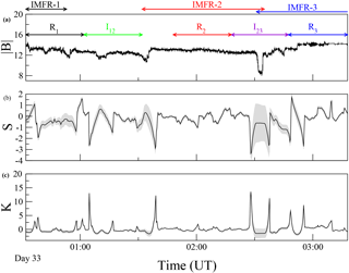
Figure 2 (a) Time series of $\left|\mathit{B}\right|$ from 00:32 to 03:18 UT on 2 February 2002. Five regions of 30 min each are highlighted using different colors: interior of IMFR-1 (R₁, black), interface region of IMFR-1 and IMFR-2 (I₁₂, green), the interior of IMFR-2 (R₂, red), the interface of IMFR-2 and IMFR-3 (I₂₃, violet), and the interior of IMFR-3 (R₃, blue). The interval of each IMFR is indicated by horizontal arrows as in Fig. 1. (b, c) Time series of the skewness S and the kurtosis K computed using a sliding overlapping window of size 10 000 data points and a window shift of 400 data points. The SD computed in each window is represented by a gray area.

The S–K parabolic relation described by Eq. (7) can be verified by computing S and K from a number of datasets corresponding to different realizations of an experiment. In the case of a time series, the parabolic relation can be tested by computing S and K using datasets extracted from the time series with sliding windows. The size of the sliding window is a critical parameter for this type of analysis. Since S and K are higher statistical moments, the number of data points inside the window should be large enough to guarantee the robust estimation of S and K. However, if the time series is divided into sliding windows with a large number of data points, then the number of (S, K) values may be insufficient to verify the parabolic relation of Eq. (7). This can be solved by defining overlapping windows; nevertheless, the overlapping cannot be too large in order to obtain a set of independent (S, K) values. To determine the optimal window size, we applied a procedure to estimate the maximum order of the statistical moment in a time series (de Wit, 2004; Miranda et al., 2013). We computed the maximum statistical order in each sliding window of size 5000 data points across the time series of Fig. 2, and a window shift of 400 data points. Then, we increased the size of the window by 1000 data points (keeping the same window shift), computed the maximum order in each window and then repeated the procedure. We found that a sliding window of size 10 000 data points is large enough for a robust estimation of moments up to the sixth order in all windows and at the same time allows a sufficient number of estimations of S an K to be obtained to test the parabolic relation of Eq. (7). Figure 2b and c show the resulting time series of S and K, respectively. The SD gives an estimation of the uncertainty of the computed S and K inside each window, and is represented using a gray area. From this figure we observe that from 02:26 to 02:35 UT the uncertainty of S and K increases due to the large variation in $\left|\mathit{B}\right|$ at the interface between IMFR-2 and IMFR-3. A similar behavior was observed in magnetic field data during an interplanetary shock event by Vörös et al. (2006). The uncertainty within sliding windows that contain the large variations in $\left|\mathit{B}\right|$ increases due to nonstationarity. Following Vörös et al. (2006), we exclude these windows from further analysis.

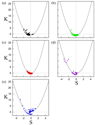
Figure 3 Kurtosis K as a function of skewness S computed using overlapping windows of size 10 000 data points and a window shift of 400 data points, for (a) the interior region of IMFR-1, (b) the interface of IMFR-1 and IMFR-2, (c) the interior of IMFR-2, (d) the interface of IMFR-2 and IMFR-3, and (e) the interior of IMFR-3. In each panel, the least-square fit with the parabolic function $K=\mathit{\alpha }{S}^{\mathrm{2}}+\mathit{\beta }$ is displayed as a dashed line (see Table 3).

Figure 3 shows K as a function of S for the five regions previously defined. A least-square fit with Eq. (7) is displayed as a dashed line. Table 3 shows the resulting fit for each region, as well as the correlation index r between the points in the scatter plot and the fitted parabolic function computed using Eq. (8). Since the interpretation of α and β is under debate (see the discussion in Sect. 5) we will focus on the computed value of r.

Table 3 The least-square fits of Eq. (7) computed from the scatter plots of Fig. 3, and the correlation index r for the five regions defined.

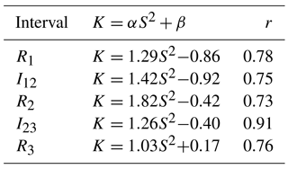
The correlation index r shown in the last column of Table 3 measures how well the data points can be adjusted by the parabolic function given by Eq. (7). All regions display r>0.5. The lowest correlation is obtained for the interval corresponding to R₂, in agreement with a visual inspection of Fig. 3c. For this interval, most of the points in Fig. 3c tend to accumulate around $(S,K)=(\mathrm{0},\mathrm{0})$, which is the value obtained for a Gaussian distribution (i.e., in the absence of coherent structures). Therefore, the interior of IMFR-2 is characterized by a low degree of non-Gaussianity and intermittency in comparison with the other intervals.

The highest value of the correlation is obtained during I₂₃ (see Table 3). Figure 3d shows that points spread near the fitted parabola and far from the (0, 0) Gaussian point. This indicates that this interval is characterized by a higher degree of non-Gaussianity. These results are in agreement with the results of Chian et al. (2016), which found that the interior of IMFR-2 has lower degrees of non-Gaussianity and phase coherence, and a nearly monofractal scaling when compared with other intervals. For the interface of IMFR-2 and IMFR-3 they observed higher degrees of non-Gaussianity and phase synchronization, and a strong departure from monofractality.

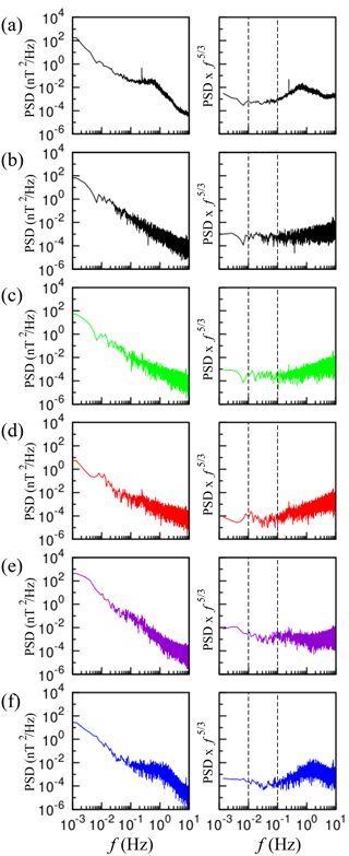
Figure 4 The power spectral density (PSD, left panels) and the compensated PSD (right panels) for (a) the time series of $\left|\mathit{B}\right|$ from 00:32 UT until 08:40 UT, (b) the IMFR-1 interior region, (c) the interface between IMFR-1 and IMFR-2, (d) the IMFR-2 interior region, (e) the interface between IMFR-2 and IMFR-3, and (f) the IMFR-3 interior region. Vertical dashed lines indicate the beginning and the end of the inertial subrange.

4.2 Time series of $\mathit{\delta }\left|\mathit{B}\right|$

Next, we investigate the S–K parabolic relation as a function of scale within the inertial subrange. The left side of Fig. 4a shows the power spectral density (PSD) as a function of frequency f of the time series of $\left|\mathit{B}\right|$ from the beginning of IMFR-1 at 00:32 UT until the end of IMFR-3 at 08:40 UT. The right side of Fig. 4a shows the compensated PSD which is the original PSD multiplied by f^5∕3 (Biskamp et al., 1999). The inertial subrange should appear as a frequency range in which the compensated PSD is almost horizontal. The following panels in Fig. 4 show the PSD and the compensated PSD for R₁, I₁₂, R₂, I₂₃ and R₃. A common frequency range in which the compensated PSD is almost horizontal for all regions is indicated by two vertical dashed lines. From Fig. 4, the inertial subrange starts at f=0.01 Hz and ends at f=0.1 Hz, which correspond to scales τ=100 s and τ=10 s, respectively.

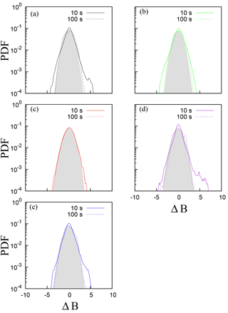
Figure 5 Probability distribution functions (PDFs) of ΔB(τ) for τ=10 s (continuous line) and τ=100 s (dashed line). (a) The interior region of IMFR-1, (b) the interface of IMFR-1 and IMFR-2, (c) the interior of IMFR-2, (d) the interface of IMFR-2 and IMFR-3, and (e) the interior of IMFR-3. A Gaussian distribution function is represented by the gray area.

The intermittent aspect of interplanetary magnetic field turbulence can be demonstrated by constructing the PDF of the normalized magnetic-field differences

$${\displaystyle }\mathrm{\Delta }B\left(\mathit{\tau }\right)={\displaystyle \frac{\mathit{\delta }B\left(\mathit{\tau }\right)-〈\mathit{\delta }B〉}{{\mathit{\sigma }}_B}},$$

where $\mathit{\delta }B\left(\mathit{\tau }\right)=\left|\mathit{B}\right(t+\mathit{\tau }\left)\right|-\left|\mathit{B}\right(t\left)\right|$, and the brackets denote the average value. Figure 5 shows the PDFs of ΔB constructed from the magnetic field fluctuations of the five regions, for τ=10 s and τ=100 s. From this figure it is clear that the PDFs are closer to a Gaussian distribution (represented by the gray area in Fig. 5) at τ=100 s (large scale), and become non-Gaussian at τ=10 s (small scale), exhibiting sharp peaks and fat tails. This figure demonstrates that magnetic field fluctuations become more intermittent as the scale τ becomes smaller.

Next, we analyze the S–K relation of ΔB(τ) at τ=10 s and τ=100 s. Figure 6a shows the time series of ΔB(τ=100 s). Figure 6b and c show the time series of S and K computed using a sliding overlapping window as in Sect. 4.1. The gray area indicates the uncertainty of the S and K values. As in Fig. 2, we observe a large uncertainty from 02:26 to 02:35 UT due to the interface between IMFR-2 and IMFR-3; therefore these S and K values are excluded from further analysis.

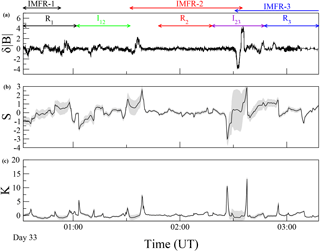
Figure 6 (a) Time series of δB(τ=100 s) from 00:00 to 04:00 UT on 2 February 2002. Five regions of 30 min each are highlighted using different colors: interior of IMFR-1 (R₁, black), interface region of IMFR-1 and IMFR-2 (I₁₂, green), the interior of IMFR-2 (R₂, red), the interface of IMFR-2 and IMFR-3 (I₂₃, violet), and the interior of IMFR-3 (R₃, blue). The interval of each IMFR is indicated by horizontal arrows as in Fig. 1. (b, c) Time series of the skewness S and the kurtosis K computed using a sliding overlapping window with the same parameters as in Fig. 2. The SD computed in each window is represented by a gray area.

Figures 7 and 8 show the S–K scatter plots for τ=100 s and τ=10 s, respectively. From these figures, we note that R₂ does not display a parabolic shape on the two selected scales. The low value of the correlation index of R₂ shown in Tables 4 and 5 confirms that the data points fit the parabolic shape poorly. This indicates that magnetic field fluctuations during R₂ are nearly Gaussian even on the smallest scale.

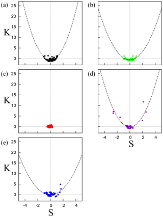
Figure 7 Kurtosis K as a function of skewness S computed from the time series of $\mathit{\delta }\left|\mathit{B}\right|\left(\mathit{\tau }\right)$, where τ=100 s. (a) The interior region of IMFR-1, (b) the interface of IMFR-1 and IMFR-2, (c) the interior of IMFR-2, (d) the interface of IMFR-2 and IMFR-3, and (e) the interior of IMFR-3. In each panel, the least-square fit with the parabolic function $K=\mathit{\alpha }{S}^{\mathrm{2}}+\mathit{\beta }$ is displayed as a dashed line (see Table 4).

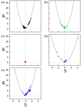
Figure 8 Kurtosis K as a function of skewness S computed from the time series of $\mathit{\delta }\left|\mathit{B}\right|\left(\mathit{\tau }\right)$, where τ=10 s. (a) The interior region of IMFR-1, (b) the interface of IMFR-1 and IMFR-2, (c) the interior of IMFR-2, (d) the interface of IMFR-2 and IMFR-3, and (e) the interior of IMFR-3. In each panel, the least-square fit with the parabolic function $K=\mathit{\alpha }{S}^{\mathrm{2}}+\mathit{\beta }$ is displayed as a dashed line (see Table 5).

Table 4 The least-square fits of Eq. (7) computed from the scatter plots of Fig. 7 (τ=100 s). The fitting function of IMFR-2 was not applicable (n/a) due to the small correlation value.

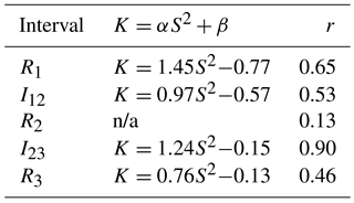
Table 5 Same as in Table 3 for τ=10 s. The fitting function of IMFR-2 was not applicable (n/a) due to the small correlation value.

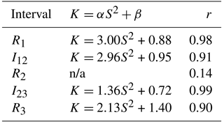
Except for R₂, all other regions show a parabolic shape at τ=100 s that is enhanced at τ=10 s, in agreement with the intermittent nature of magnetic field turbulence. Magnetic field fluctuations in the solar wind turbulence display a scale dependence in which they become intermittent as the scale becomes smaller, within the inertial subrange, due to rare, large-amplitude coherent structures. As a consequence, statistics of magnetic field fluctuations such as the PDFs of the ΔB (Fig. 5) departure from Gaussian statistics as τ decreases. By comparing the values of the correlation index shown in Table 4 for τ=100 s with those of Table 5 for τ=10 s we note that, for each region, the correlation r increases on the smallest scale, confirming that the S–K parabolic relation displays scale dependence within the inertial subrange.

The highest correlation value for τ=100 s (Table 4) corresponds to I₂₃. This indicates that the ongoing magnetic reconnection occurring in this region can act as a source of non-Gaussianity and intermittent turbulence even on the largest scale. At τ=10 s, Table 5 shows that r=0.99 at I₂₃ and r=0.98 at R₁. Small-scale current sheets were detected in these two intervals by Chian et al. (2016) and are responsible for intermittency and non-Gaussian fluctuations. Our result demonstrates that they are also responsible for the enhancement of the S–K parabolic relation. Note that there are points in Fig. 8d that are further away from the (0, 0) Gaussian point, compared to Fig. 8a. This means that while the scatter plots of R₁ and I₂₃ are highly correlated with Eq. (7), the numerical values of S and K, which measure the degree of asymmetry and non-Gaussianity respectively, can be higher at I₂₃.

5 Discussion

A theoretical explanation of the parabolic relation between the skewness and kurtosis of turbulent fluids and plasmas is still an open question. Sura and Sardeshmukh (2007) proposed a nonlinear Langevin equation with external forcing that can account for the parabolic relation between S and K. Krommes (2008) extended this model to include self-generated internal instabilities in plasmas. Sattin et al. (2009) argued that a parabolic relation can be obtained as a natural consequence of a number of constraints expected to be met for most physical systems. Guszejnov et al. (2013) proposed a simplified model of a synthetic intermittent time series, constructed from a random number of coherent structures with random amplitudes embedded in a background Gaussian noise, and demonstrated that their model can predict a S–K parabolic relation. A similar study was performed by Bergsaker et al. (2015) using a model of coherent plasma flux events.

Although a theoretical explanation of the S–K relation is still unclear, there is a consensus that the parabolic shape is due to non-Gaussianity related to coherent structures, whereas points near $(S,K)=(\mathrm{0},\mathrm{0})$ correspond to Gaussian fluctuations. This is confirmed by models of synthetic time series. For example, Sandberg et al. (2009) proposed a model of intermittent time series which consists of a superposition of Gaussian and non-Gaussian random fluctuations. Their model includes a parameter that measures the deviation from Gaussianity. The resulting PDF derived from their model displays asymmetric long tails that reproduce measured distributions of plasma density fluctuations in plasma magnetic confinement devices (Antar et al., 2001, 2003) as well as distributions of X-ray emissions detected from accretion disks (Sandberg et al., 2009). Their model also leads to a parabolic relation between S and K. Bergsaker et al. (2015) observed a transition from a parabolic shape to the $(S,K)=(\mathrm{0},\mathrm{0})$ point by increasing the intensity of the Gaussian noise in their model of synthetic time series, constructed by adding deterministic fluctuations and Gaussian noise. However, a quantification of the parabolic shape is needed for an objective comparison between different datasets. We have found that the computation of the correlation index r allows time series dominated by either Gaussian and non-Gaussian fluctuations to be clearly distinguished. Despite the simplicity of this approach, it represents an alternative way to compare the degree of non-Gaussianity due to asymmetry and fat tails in the PDFs of different datasets, and can be applied to observational data and results from numerical simulations.

The stochastic model of a time series proposed by Sandberg et al. (2009) assumes that the non-Gaussian fluctuations arise from a quadratic nonlinear term. By increasing the degree of non-Gaussianity the skewness and the kurtosis converge to extreme values: $S=\pm \mathrm{2}\sqrt{\mathrm{2}}$ and K=12. This means that experimental data governed by nonlinear processes of quadratic order should lead to S–K scatter plots with $S\in [-\mathrm{2}\sqrt{\mathrm{2}},\mathrm{2}\sqrt{\mathrm{2}}]$ and K<12. The scatter plots shown in Fig. 3a, c and e seem to agree with these limits; however, in Fig. 3d there are some points in which $S<-\mathrm{2}\sqrt{\mathrm{2}}$. Sandberg et al. (2009) also propose that processes described by higher-order nonlinearities can result in S–K parabolic shapes with S outside the interval $[-\mathrm{2}\sqrt{\mathrm{2}},\mathrm{2}\sqrt{\mathrm{2}}]$, which can explain the behavior of $\left|\mathit{B}\right|$ during the magnetic reconnection occurring in the I₂₃ interval.

In the previous sections we showed and discussed the value of the correlation index measuring how well the S–K scatter plots fit with a parabola. As mentioned before, there is no agreement on the interpretation of the coefficients α and β in Eq. (7). Sattin et al. (2009) argues that the coefficients are not likely to offer relevant information about the underlying process. However, Guszejnov et al. (2013) discussed an interpretation of the α and β coefficients based on their model of a synthetic time series. The value of the α coefficient depends on the statistics of the fluctuations due to coherent structures and is not necessarily constant in time. For the β coefficient, if the number of coherent structures in a time series can be represented as random independent variables that follow a Poisson distribution function (which models the occurrence of rare events), then β=3. Deviations from this value can be interpreted as a departure from the independence assumption, which means that there is interaction among coherent structures (Guszejnov et al., 2013). Since we define kurtosis to be the flatness minus three, the previous statement is equivalent to say that deviations from β=0 are due to interacting coherent structures. From Table 3, we note that all intervals have nonzero values of β. Recall that this event is characterized by a rope–rope magnetic reconnection involving IMFR-2 and IMFR-3, with formation of a bifurcated current sheet acting as a source of intermittent turbulence (Chian et al., 2016). The interaction between the small-scale IMFR-2 and the medium-scale IMFR-3 occurring during this event gives support for the interpretation of the β parameter by Guszejnov et al. (2013).

Vörös et al. (2006) demonstrated that the S–K parabolic relation is also observed for time series of two-point differences of $\left|\mathit{B}\right|$ in the solar wind. They showed that this relation is enhanced in the presence of large-scale events such as interplanetary shocks, whereas for nonshock intervals, the parabolic relation is not observed. In this case the S–K parabolic relation represents a signature of direct coupling between large-scale structures (interplanetary shocks) and small-scale intermittency. Our results indicate that the S–K parabolic relation is present during reconnection between a small-scale IMFR with a duration of ∼60 min and a medium-scale IMFR with a duration of ∼7 h (see Table 1). The only region in which the parabolic relation is not observed is in the interior of IMFR-2. This region was found to have a low degree of intermittency and nearly monofractal scaling. Therefore, our results are in accordance with cross-scale coupling between IMFR scales and scales within the inertial subrange.

6 Conclusions

In this paper we investigated the relation between the skewness and the kurtosis during a triple-IMFR event on 2 February 2002. This event was divided into five regions, namely, the interior of IMFR-1, the interface of IMFR-1 and IMFR-2, the interior of IMFR-2, the interface of IMFR-2 and IMFR-3, and the interior of IMFR-3. We then computed the skewness S and the kurtosis K of $\left|\mathit{B}\right|$ using a sliding window, and showed that the scatter plots of K as a function of S display a parabolic shape for all regions. The highest value of the correlation index computed by a least-square fit between the (S,K) values and Eq. (7) occurs at the interface of IMFR-2 and IMFR-3. This region was found to be the source of intermittent turbulence due to a magnetic reconnection between the small-size IMFR-2 and the medium-size IMFR-3 (Chian et al., 2016). Therefore, the enhanced S–K parabolic relation is related to non-Gaussian fluctuations due to coherent structures emerging from intermittent turbulence generated via magnetic reconnection. The lowest value of the correlation index was obtained at the interior of IMFR-2, in agreement with the results of Chian et al. (2016), who found that this region is characterized by a low degree of non-Gaussianity and phase synchronization, and nearly monofractal scaling.

We also analyzed the S–K relation using two-point differences of $\left|\mathit{B}\right|$ on two different scales within the inertial subrange. By computing the compensated PSD we selected an interval of frequencies in which all regions exhibit $-\mathrm{5}/\mathrm{3}$ scaling corresponding to the inertial subrange and selected two timescales representing the largest scale (τ=100 s) and the smallest scale (τ=10 s) within the inertial subrange. We found that the scatter plot of IMFR-2 on the largest scale (τ=100 s) and on the smallest scale (τ=10 s) accumulate around the $(S,K)=(\mathrm{0},\mathrm{0})$ point. The least-square fit with Eq. (7) results in a low correlation index, which confirms that magnetic field fluctuations in this region are nearly Gaussian. All other regions displayed parabolic shapes. At τ=100 s, the correlation index is high for the interface of IMFR-2 and IMFR-3, indicating that the magnetic reconnection that occurs in this region can generate non-Gaussian fluctuations on the largest scale. On the smallest scale, the correlation index is higher for two regions, namely, the interior of IMFR-1 and the interface of IMFR-2 and IMFR-3. This result can be due to non-Gaussian fluctuations resulting from small-scale current sheets detected within these regions (Chian et al., 2016). Our analysis indicates that the S–K parabolic relation observed in interplanetary magnetic field turbulence is enhanced on small scales within the inertial subrange.

Our findings give support to the conclusion by Chian et al. (2016) that rope–rope magnetic reconnection acts as a source of interplanetary intermittent turbulence and suggest that magnetic reconnection is responsible for non-Gaussian PDFs with asymmetric shapes and fat tails. The results are also in agreement with the results of Vörös et al. (2006) in that the S–K parabolic relation is a signature of direct coupling between IMFR scales and small-scale intermittency.