Multi-scale analysis of compressible fluctuations in the solar wind

Compressible plasma turbulence is investigated in the fast solar wind at proton kinetic scales by the combined use of electron density and magnetic field measurements. Both the scale-dependent cross-correlation (CC) and the reduced magnetic helicity (σ_m) are used in tandem to determine the properties of the compressible fluctuations at proton kinetic scales. At inertial scales the turbulence is hypothesised to contain a mixture of Alfvénic and slow waves, characterised by weak magnetic helicity and anti-correlation between magnetic field strength B and electron density n_e. At proton kinetic scales the observations suggest that the fluctuations have stronger positive magnetic helicities as well as strong anti-correlations within the frequency range studied. These results are interpreted as being characteristic of either counter-propagating kinetic Alfvén wave packets or a mixture of anti-sunward kinetic Alfvén waves along with a component of kinetic slow waves.

Keywords. Interplanetary physics (MHD waves and turbulence)

1 Introduction

The solar wind is a magnetised collisionless plasma outflowing from the Sun. Measurements of several parameters show irregular fluctuations over several decades in scale (Bruno and Carbone, 2013). The dominant component of the energy in these fluctuations is in the directions perpendicular to the mean magnetic field direction $\mathit{\delta }{\mathit{B}}_{⟂}\gg \mathit{\delta }{\mathit{B}}_{\parallel }$ (Bieber et al., 1996). However, the solar wind plasma is also weakly compressible with non-negligible fluctuations in magnetic field strength (δB_∥) and density (δn) (Tu and Marsch, 1994).

Turbulence is an inherently nonlinear process. However, there is evidence that the plasma is in a state of “critical balance” (Goldreich and Sridhar, 1995). This is a state where the nonlinear timescale and the linear timescale constantly evolve toward being equal. Therefore, even when nonlinearity is strong, the linear terms are of the same order and the system may retain some properties of linear wave modes; this is often termed the quasilinear premise (Klein et al., 2012). Several multi-spacecraft observations of the solar wind have revealed that the fluctuations at proton kinetic scales typically have low intrinsic propagation speeds in the plasma frame. This result has been interpreted as evidence of kinetic Alfvén waves (KAWs) (Sahraoui et al., 2010), as coherent structures which are predominantly advected with the bulk velocity (Perrone et al., 2017), as a combination of KAW turbulence and coherent structures (Roberts et al., 2013, 2015), or as nonlinear modes where wave–wave interactions have broadened the dispersion relation diagram (Narita and Motschmann, 2017; Roberts et al., 2017). Kinetic slow waves (KSWs) are the kinetic counterpart of the magnetohydrodynamic (MHD) slow mode when it develops a large perpendicular wave number, and it shares many properties with the KAW, such as a similar dispersion relation and anti-correlated fluctuations in magnetic field and density (Klein et al., 2012; Narita and Marsch, 2015). The distinct identification of either KAWs or KSWs using only the dispersion relation diagram is challenging given the error in the measurements. This result motivates further study of the same interval with techniques which can distinguish between KAWs and KSWs.

The goal of this study is to identify the linear wave more uniquely, not only using the dispersion relation diagram but also using the correlation between magnetic field and electron density as well as the helical sense of magnetic field fluctuations. Magnetic helicity was first proposed by Matthaeus and Goldstein (1982) and often gives a non-zero signature on ion kinetic scales (Leamon et al., 1998). The variation in magnetic helicity has also been investigated as a function of the angle between the magnetic field direction and the bulk flow direction giving a positive value at ${\mathit{\theta }}_{\mathit{B}\mathit{V}}\sim \mathrm{90}{}^{\circ }$ and a negative at ${\mathit{\theta }}_{\mathit{B}\mathit{V}}\sim \mathrm{0}{}^{\circ }$ (He et al., 2011; Podesta and Gary, 2011). This has been interpreted as evidence of the existence of quasi-perpendicular KAWs (Howes and Quataert, 2010) in addition to quasi-parallel ion cyclotron (He et al., 2011; Podesta and Gary, 2011; Klein et al., 2014) waves. However, these observations are subject to an ambiguity as a helical sense of a wave can be opposite depending on whether the plasma wave is propagating up- or downstream; which motivates further analysis through an investigation of the correlation of the compressible fluctuations with one another.

Ion Bernstein waves (IBWs) exhibit positive correlations between n_e and B, while KAW/KSWs both exhibit anti-correlations (Klein et al., 2012; Zhao et al., 2014). The electron density is estimated from the spacecraft potential (Pedersen et al., 2001; Kellogg and Horbury, 2005), which has a sufficient time resolution to study proton kinetic scales. Meanwhile, magnetic helicity can be used to differentiate between KAWs and KSWs which have opposite helicities and polarisations (Zhao et al., 2014). Typically in the solar wind, B and n_e are anti-correlated on fluid scales (Howes et al., 2012), and also down to kinetic scales (Kellogg and Horbury, 2005; Yao et al., 2011), which have been interpreted as KSWs or pressure-balanced structures (the undamped oblique limit of the KSWs).

2 Weakly compressible event

A data interval which was taken by the Cluster (Escoubet et al., 2001) spacecraft when they were in an interval of solar wind and which is uncontaminated from the electron foreshock is analysed. The mean angle that the solar wind makes with the solar wind bulk flow is large (${\mathit{\theta }}_{\mathit{v}\mathit{B}}>\mathrm{60}{}^{\circ }$) suggesting that the plasma is not connected to the electron foreshock. Furthermore, the electric field spectrogram from the WHISPER (Waves of High Frequency and Sounder for Probing of Density by Relaxation) instrument (Décréau et al., 1997) is quiet, with no signatures of foreshock waves. The large value of θ_vB also allows us to neglect considering any contributions of quasi-parallel waves (e.g. He et al., 2011) in the analysis. The mean bulk speed of the solar wind is 655±15 km s⁻¹, the mean proton density is low 2.8±0.2 cm⁻³, and plasma $\mathit{\beta }=\mathrm{0.85}\pm \mathrm{0.29}$. There are no interplanetary coronal mass ejections or stream interaction regions recorded at the time of the interval, and the large scale from Active Composition Explorer (ACE) data (not shown) suggests that this interval can be regarded as typical of the fast solar wind (see Roberts et al., 2015).

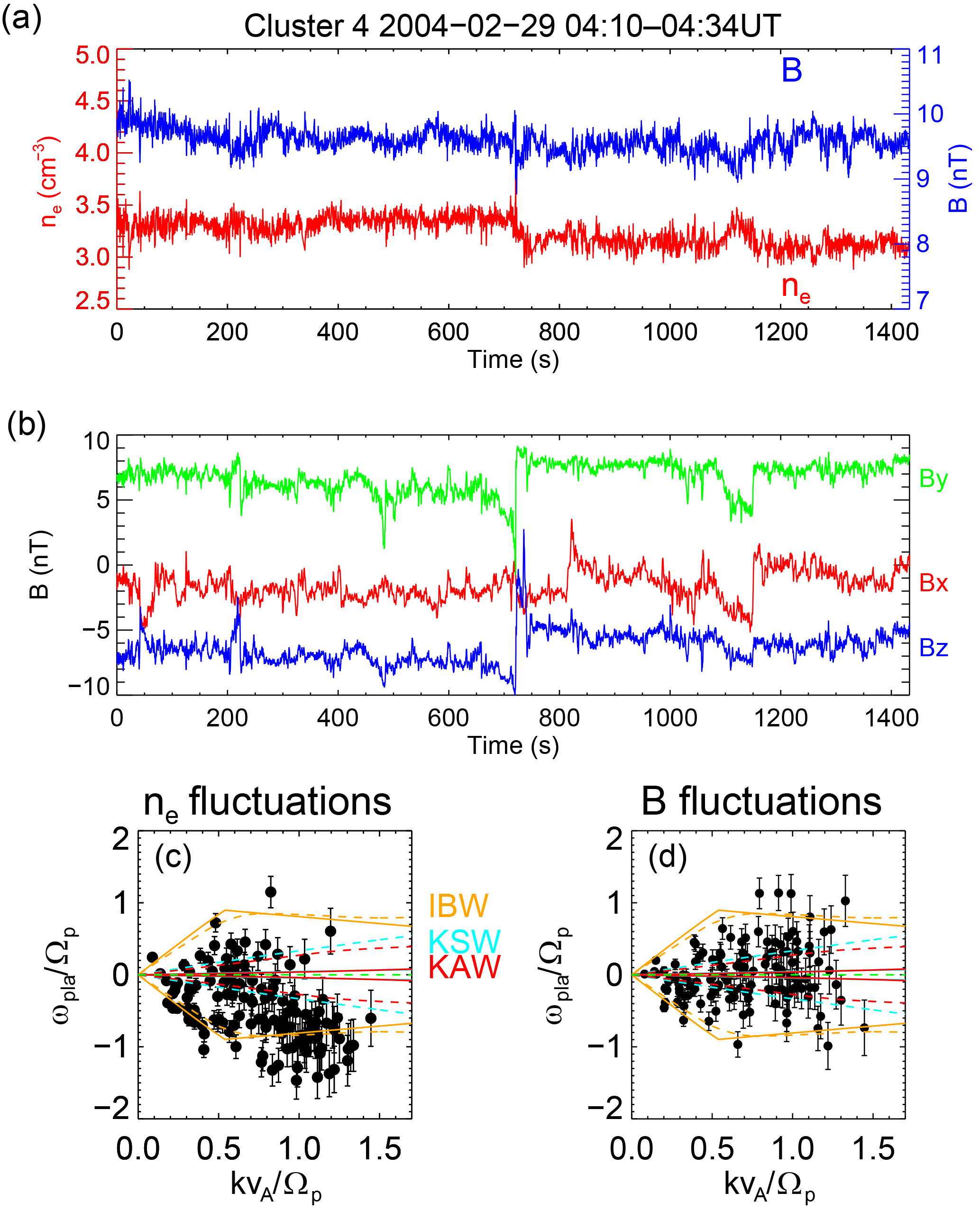
Figure 1 (a) Time series of the density (red) and the magnetic field strength (blue) fluctuations from the Cluster 4 spacecraft. (b) Time series of the magnetic field components in the GSE co-ordinate system. (c) Dispersion relation diagram of the electron density fluctuations (d) compressible magnetic fluctuations. Theoretical dispersion relations for advected structures (green), KAWs (red), KSWs (cyan) and IBWs (orange) for propagation angles ${\mathit{\theta }}_{\mathit{k}{\mathit{B}}_{\mathbf{0}}}$ = 88^∘ and 75^∘ (solid lines).

Magnetic field data are obtained from the Fluxgate magnetometer (FGM) instrument (Balogh et al., 2001) sampled at 22 Hz, and electron density data are obtained by calibrating the spacecraft potential sampled at 5 Hz, which is measured by the Electric Fields and Waves (EFW) instrument (Gustafsson et al., 1997).

The spacecraft potential is subject to a strong spin effect at 0.25 Hz and charging effects due to different parts of the spacecraft being illuminated. To remove these fluctuations we use the method presented in Roberts et al. (2017) to construct an empirical model of the spacecraft charging as a function of the phase angle. This allows the fluctuations in the spacecraft potential due to solar illumination to be removed, leaving only fluctuations due to density fluctuations. This is effective up to 1.0 Hz, above which high-frequency spikes remain and instrumental noise also becomes significant.

In Fig. 1a the electron density n_e is given in red, and the magnitude of the magnetic B field is given in blue, and both show the presence of weakly compressible fluctuations. Several small regions can be seen to demonstrate an anti-correlation of these two quantities, most notably near 1100 s. Figure 1b shows the components of the magnetic field in geocentric solar ecliptic (GSE) co-ordinates, where x_GSE points from the Earth towards the Sun and z_GSE points to the ecliptic north.

The dispersion relation diagrams of compressible magnetics and density obtained from the interval used in this study are shown in Fig. 1c and d. These are derived by the application of the multi-point signal resonator technique (Narita et al., 2011), which allows the most energetic wave vector k to be identified at each spacecraft frequency ω_sc. The corresponding plasma frame frequency can be obtained from the equation ${\mathit{\omega }}_{\mathrm{pla}}={\mathit{\omega }}_{\mathrm{sc}}-\mathit{k}\cdot \mathit{v}$. Further details can be obtained in Roberts et al. (2017). Figure 1c and d also show the theoretical linear dispersion curves for the KAWs, IBWs and KSWs for plasma β=0.85 (ratio of thermal to magnetic pressure). A green dashed line at ω=0 denotes the expectation for a static structure. The rest-frame frequencies of the fluctuations ω_pla∕Ω_p show a lot of scatter from the theoretical curves, and the error bars are significant. Moreover, the theoretical expectations for both KAWs and KSWs are very close to one another for angles close to 90^∘. This motivates the analysis of the time interval with correlations and the magnetic helicity.

To obtain a multi-scale picture, we perform a cross-correlation and magnetic helicity based on wavelet analysis (Torrence and Compo, 1998), which allows the relationship between the two signals to be analysed in time and in scale (frequency).

3 Correlation and helicity analysis

3.1 Estimators

The wavelet cross-correlation is given in Eq. (1), where ${\stackrel{\mathrm{̃}}{n}}_{\mathrm{e}}$ and $\stackrel{\mathrm{̃}}{B}$ are the complex wavelet coefficients for the electron density and the magnitude of the magnetic field respectively, while the Re denotes the real part and the asterisk denotes the complex conjugate. The value of CC varies between −1 (full anti-correlation) and +1 (full correlation). In order to compare the magnetic field data with the electron density data in this way, the magnetic field data are resampled at 5 Hz.

$$\begin{array}{}\text{(1)}& {\mathrm{CC}}_{n,B}(t,f)={\displaystyle \frac{\text{Re}\left({\stackrel{\mathrm{̃}}{n}}_{\mathrm{e}}(t,f){\stackrel{\mathrm{̃}}{B}}^{*}(t,f)\right)}{\left|{\stackrel{\mathrm{̃}}{n}}_{\mathrm{e}}\right(t,f\left)\right|\left|\stackrel{\mathrm{̃}}{B}\right(t,f\left)\right|}}\end{array}$$

As a further diagnostic tool for the magnetic fluctuations, we also analyse the magnetic helicity. The magnetic helicity is the spatial rotation sense of the magnetic fluctuation about the wave vector. We use the definition in Eq. (2), where the tilde denotes the wavelet coefficients of the GSE components of the magnetic field in GSE and Im denotes imaginary parts.

$$\begin{array}{}\text{(2)}& {\mathit{\sigma }}_{\mathrm{m}}(t,f)={\displaystyle \frac{\text{Im}\left({\stackrel{\mathrm{̃}}{B}}_y^{*}(t,f){\stackrel{\mathrm{̃}}{B}}_z(t,f)\right)}{\left|{\stackrel{\mathrm{̃}}{B}}_y\right(t,f){|}^{\mathrm{2}}+|{\stackrel{\mathrm{̃}}{B}}_z(t,f){|}^{\mathrm{2}}}}\end{array}$$

It is important to note that this definition assumes that the wave vector k is along −x_GSE (approximately along the flow) and also implicitly assumes Taylor's hypothesis, i.e. that there is no temporal change. Thus, the magnetic helicity varies between −1 and +1 and for this definition can be regarded as being the same as polarisation (temporal rotation sense of the fluctuations with respect to the magnetic field). Thus, positive (negative) helicity is indicative of a polarisation sense in the right- (left-) handed direction in the direction of electron (proton) gyration. However, an important caveat of this method is that it does not contain information about the propagation direction of the fluctuations. As such a right-hand polarised wave can give the appearance of a left-handed wave if the propagation direction is reversed (Narita et al., 2009).

3.2 Results

Figure 2a shows the cross-correlation spectra, where the white line denotes the cone of influence associated with the wavelet transform (Torrence and Compo, 1998); below this line the spectrum is unreliable due to edge effects. The spectrum is dominated by anti-correlated fluctuations throughout with small regions of sporadic positive correlation peppering the spectrum. This suggests that IBWs are not present or are only present for very brief times.

Figure 2b shows the magnetic helicity spectrum. The value of the helicity shows a mix of different values on fluid scales $f\in [\mathrm{0.01},\mathrm{0.2}]$ and a general increase on kinetic scales $f\in [\mathrm{0.4},\mathrm{2}]$ towards a value of σ_m∼0.5 near 1 Hz. At spacecraft frame frequencies of f_sc≥1.0 Hz and f_sc≥2 Hz, instrumental noise becomes significant in the spacecraft potential and in the magnetic field data respectively. Another important issue is that of aliasing, which affects high frequencies and can artificially reduce the value of the helicity (e.g. Klein et al., 2014). However, in previous studies of the helicity, the sampling rates of magnetic field instruments is much lower than for Cluster, and the data presented here are not as strongly affected. Aliasing would be expected to significantly affect frequencies above 5.5 Hz in the helicity measurement and 1.25 Hz for the cross-correlation; however, we are already near the instrument noise levels.

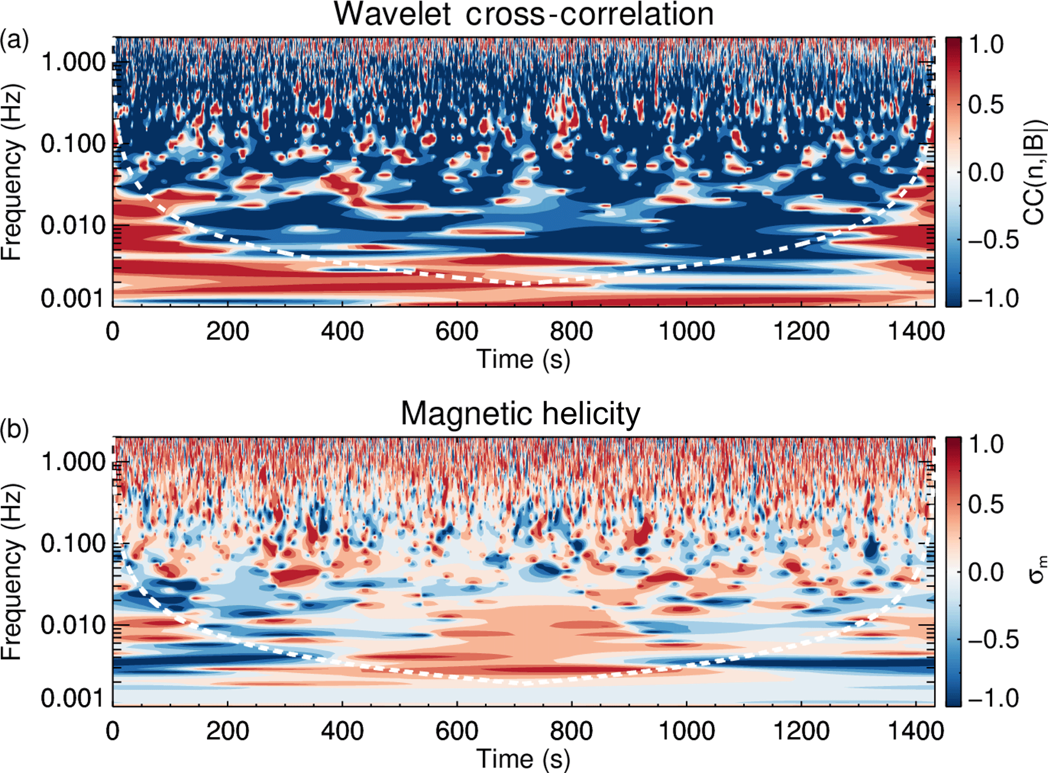
Figure 2 (a) Wavelet cross-correlation of the electron density and magnetic field strength. (b) Magnetic helicity. The white dashed line denotes the cone of influence region where the spectrum is unreliable due to edge effects.

The negative cross-correlation signature and negative helicity on fluid scales is likely to be due to MHD slow waves (Howes et al., 2012) or pressure-balanced structures (Yao et al., 2011). However, there are regions on fluid scales which have positive helicity and negative cross-correlation which could be due to a fluid-scale Alfvén wave. On ion kinetic scales, more regions of positive cross-correlation appear, but they are still less numerous than the negatively correlated regions, while the magnetic helicity increases and is predominantly above 0.

The mean value at each frequency for the cross-correlation and the helicity is given in Fig. 3a. The cross-correlation remains negative throughout, with a minimum near 0.5 Hz, and then remains at a similar value until Taylor-shifted proton scales, and then it increases before being influenced by noise near 2 Hz. The magnetic helicity is close to 0 on fluid scales and then increases at 0.5 Hz, reaching a maximum plateau at the Taylor-shifted scales (denoted by the green and purple vertical line) before decreasing. Analysis of the helicity from the search coil magnetometer (SCM) (Cornilleau-Wehrlin et al., 2003) is shown as the dotted red line in Fig. 3a. The SCM is more sensitive than FGM and is sampled at 25 Hz. The data from SCM show that the helicity is indeed lower at $\mathrm{2}<f_{\mathrm{sc}}<\mathrm{5.5}$ Hz, and due to the higher sampling rate and sensitivity, this is not an artefact of aliasing or noise.

To understand the relative importance of the competing wave modes, we use the thresholds in Table 1 to find the relative occurrence rates. These thresholds are motivated by what is expected for each wave mode from linear theory (e.g. Klein et al., 2012) and assume anti-sunward propagation.

Table 1 Table of the thresholds used to identify different wave modes for fluid (fl) and kinetic (ki) scales.

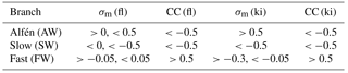
Figure 3b shows the ratio r of data points which reach the thresholds outlined in Table 1 to the total number of data points. On large scales the plasma is dominated by MHD Alfvén waves and slow waves. However, as we approach proton scales, these both decrease and this method clearly identifies that the dominant type of fluctuation on proton scales is the KAW, with very few points at proton kinetic scales reaching the thresholds for KSWs or IBWs. At the highest frequencies there is a small increase in both of these wave modes; however, it is unclear whether this is true or related to the instrumental noise. It should be noted that a sunward-propagating KSW would in this case produce the same signature as the KAW; therefore, in interpreting the data in Roberts et al. (2017) and Fig. 1c and d this mixture of two waves may explain the scatter seen. Moreover, even though some points in Fig. 1c and d, may agree better with the curves for IBWs as there is no significant signature in the cross-correlation, this is most likely due to wave–wave interactions between individual KAW packets or KAWs and KSWs (Narita and Motschmann, 2017; Roberts et al., 2017). It is also interesting to note that while the KAW dominates both other wave modes, the majority of the fluctuations do not fall into the thresholds in Table 1.

Figure 3 (a) Mean values at each spacecraft frame frequency for the helicity (red) and the wavelet cross-correlation (blue). Light shaded areas denote 1 standard deviation, and the dashed red line denotes the helicity from the search coil magnetometer. (b) Ratio of data points meeting the thresholds to the total number of points in the interval, which are defined in Table 1. The solid lines denote the ratio of points that meet the kinetic thresholds. Lighter dotted lines denote the ratio for the fluid thresholds.

4 Conclusions

To summarise: compressible fluctuations in an interval of fast solar wind were investigated using high time resolution density and magnetic field data. Cross-correlation analysis supports the hypothesis that the compressible component is more characteristic of KAW turbulence than magnetosonic turbulence on these scales. Magnetic helicity measurements also suggest that highly compressible KSWs may also be present on these scales and may explain some results presented by Roberts et al. (2017), where the dispersion plot for the compressible component was found to be more scattered than the incompressible component.

A plausible scenario is that on inertial scales the compressible component is dominated by Alfvén and slow waves which are passively cascaded where the energy cascade rate is dependent on the Alfvén wave frequency rather than on the slow wave frequency, as discussed by Schekochihin et al. (2009). While at proton kinetic scales, these KAWs and KSWs interact and result in a dispersion curve that is a superposition of different modes; a single mode cannot be definitively identified in Fig. 1c and d. Moreover, the helicity and the cross-correlation approach maxima and minima respectively. Then the KSWs are damped strongly, leading to an increase in the CC, and the KAWs begin to damp soon after reducing the helicity. Such a scenario explains the evolution of the cross-correlation and magnetic helicity from large to small timescales in Fig. 2. An alternative is that the compressible component on inertial scales is dominated by slow waves which are then damped, while on kinetic scales, the compressible component comes solely from KAWs. In this case the times with opposite helicity are KAWs propagating in the sunward direction. Therefore, some KAWs may then be misinterpreted as KSWs should they propagate in the sunward direction. To overcome this, a scale-dependent propagation direction is needed as well as the other quantities such as helicity and cross-correlations. Alternatively, the Alfvén ratio is another possibility which can distinguish between KAW and KSWs without the need for the propagation direction (Zhao et al., 2014).