Satellite observations of middle atmosphere–thermosphere vertical coupling by gravity waves

Atmospheric gravity waves (GWs) are essential for the dynamics of the middle atmosphere. Recent studies have shown that these waves are also important for the thermosphere/ionosphere (T/I) system. Via vertical coupling, GWs can significantly influence the mean state of the T/I system. However, the penetration of GWs into the T/I system is not fully understood in modeling as well as observations. In the current study, we analyze the correlation between GW momentum fluxes observed in the middle atmosphere (30–90 km) and GW-induced perturbations in the T/I. In the middle atmosphere, GW momentum fluxes are derived from temperature observations of the Sounding of the Atmosphere using Broadband Emission Radiometry (SABER) satellite instrument. In the T/I, GW-induced perturbations are derived from neutral density measured by instruments on the Gravity field and Ocean Circulation Explorer (GOCE) and CHAllenging Minisatellite Payload (CHAMP) satellites. We find generally positive correlations between horizontal distributions at low altitudes (i.e., below 90 km) and horizontal distributions of GW-induced density fluctuations in the T/I (at 200 km and above). Two coupling mechanisms are likely responsible for these positive correlations: (1) fast GWs generated in the troposphere and lower stratosphere can propagate directly to the T/I and (2) primary GWs with their origins in the lower atmosphere dissipate while propagating upwards and generate secondary GWs, which then penetrate up to the T/I and maintain the spatial patterns of GW distributions in the lower atmosphere. The mountain-wave related hotspot over the Andes and Antarctic Peninsula is found clearly in observations of all instruments used in our analysis. Latitude–longitude variations in the summer midlatitudes are also found in observations of all instruments. These variations and strong positive correlations in the summer midlatitudes suggest that GWs with origins related to convection also propagate up to the T/I. Different processes which likely influence the vertical coupling are GW dissipation, possible generation of secondary GWs, and horizontal propagation of GWs. Limitations of the observations as well as of our research approach are discussed.

Keywords. Ionosphere (ionosphere–atmosphere interactions)

1 Introduction

The thermosphere/ionosphere (T/I) system is an essential part of the Earth's atmosphere. Via interaction with the T/I system, space weather can significantly influence the telecommunication, navigation systems as well as space technology (Belehaki et al., 2009; Yiğit et al., 2016). The T/I is influenced by processes from above (e.g., solar wind, magnetosphere) as well as from below. One of the significant processes from below is vertical coupling by atmospheric waves. These atmospheric waves have a wide range of horizontal scales extending from mesoscale (gravity waves) to global scale (tides, planetary waves). In recent years, it has been increasingly acknowledged that vertical coupling by atmospheric waves from below plays an important role in energy and momentum balance of the T/I. A number of review papers regarding this issue have been presented (e.g., Kazimirovsky et al., 2003; Altadill et al., 2004; Laštovička, 2006, 2009; Forbes, 2007; Yiğit and Medvedev, 2015, 2016; Yiğit et al., 2016).

Vertical coupling between middle atmosphere and ionosphere by planetary waves has important effects on the dynamics of the ionosphere (e.g., see the reviews of Laštovička, 2006, 2009, and references therein). Planetary waves cannot directly propagate to the F-region altitudes. Some potential mechanisms of the indirect propagation, as summarized by Laštovička (2006), are vertical plasma drift (due to planetary wave modulation of the E-region dynamo) (Pancheva et al., 1994), tides (Laštovička and Šauli, 1999), gravity waves (e.g., Meyer, 1999), turbopause region properties or composition changes at the base of the thermosphere.

Recently, particular attention has been paid to the effects of tides on the T/I. For example, the well-known zonal “wave 4” structure has been observed in different parameters of the T/I (e.g., Häusler et al., 2007; Oberheide and Forbes, 2008; Shiokawa and Oberheide, 2009). Since then, a number of observational studies focusing on vertical coupling by tides have been conducted (e.g., Forbes et al., 2009; Oberheide et al., 2009; Liu et al., 2009; Kwak et al., 2012). Further, advances in observations and physical understanding have motivated and successfully led to a more realistic representation of tides in global models (e.g., Miyoshi et al., 2009; Jin et al., 2011; Pancheva et al., 2012; Leonard et al., 2012; Yamazaki and Richmond, 2013; Häusler et al., 2014).

Among atmospheric waves, gravity waves (GWs) possess smaller scales and a broad spectrum. Gravity waves are mostly generated in the lower atmosphere and, while propagating upwards, their amplitudes grow exponentially due to the exponential decrease in the air density. Once GWs dissipate (e.g., encountering critical wind levels, reaching amplitude saturation) they deposit their energy and momentum, accelerate or decelerate the background flow and therefore can significantly influence the dynamics of the atmosphere. The essential role of GWs in the middle atmosphere is widely acknowledged (e.g., see the review of Fritts and Alexander, 2003; Alexander et al., 2010; Becker, 2011). Due to the small scales, GWs challenge both observation and global modeling. Very often, effects of GWs need to be parameterized in the global models (McLandress, 1998; Yiğit et al., 2008; Geller et al., 2013).

GWs are important not only for the middle atmosphere, but also for the T/I. For example, they contribute to the formation of traveling ionospheric disturbances (TIDs) (e.g., Hines, 1960; Huang et al., 1994; Kirchengast et al., 1995; Vadas and Liu, 2009). In addition, it has been shown that there exists correlation between TIDs and sporadic E layers (Tsunoda, 2006), and the variations of sporadic E layers are influenced by both tides (e.g., Arras et al., 2009) and GWs (e.g., Woodman et al., 1991). Theoretical studies showing the importance of GWs in the T/I are presented by Vadas and Fritts (2005), Vadas and Fritts (2006), Vadas (2007), Fritts and Vadas (2008) and Yiğit et al. (2008). In particular, using the whole atmosphere GW parameterization of Yiğit et al. (2008) incorporated into the CMAT2 general circulation model, Yiğit et al. (2009) showed that GWs have a significant dynamic effect on the T/I. They showed that the mean GW drag can be as strong as ion drag. Further, the total heating effect due to GWs is comparable with the Joule heating, and the total cooling effect is comparable with the cooling by molecular thermal conduction (Yiğit and Medvedev, 2009). Using the same model, Yiğit and Medvedev (2010) have shown that GW propagation and dissipation in the thermosphere exhibit a distinct solar cycle variation, while Yiğit and Medvedev (2012) and Yiğit et al. (2014) have shown that during sudden stratospheric warmings (SSWs), GW distributions and their drag in the T/I can be directly impacted by GWs from the middle atmosphere. These results are confirmed by global models with resolved GWs (Miyoshi et al., 2014; Liu et al., 2014). In addition, GWs can also induce planetary waves and tides in the T/I (e.g., Laštovička, 2006; Hoffmann et al., 2012, and references therein). Recently, Yiğit and Medvedev (2017) showed that GWs can influence the migrating diurnal tide in the T/I.

Although many advances have been achieved by recent studies focusing on vertical coupling by GWs between the middle atmosphere and the T/I, the mechanism of this coupling is not fully understood and open issues remain (e.g., see the review of Yiğit and Medvedev, 2015, 2016; Yiğit et al., 2016). Modeling studies using GCMs provide insights into physical processes and are helpful for interpreting observations. However, the spatial and temporal resolution of GCMs is too coarse to fully resolve GWs and their sources, and even resolving a major part comes with high computational costs. The parametrization schemes employed to take into account the effects of the unresolved GWs are strongly simplified. For instance, except for orography, even the coupling to physical GW source processes is missing in many models. Initial parameters of the GW parametrization schemes have to be chosen and the mean wind and temperature fields produced by the GCM are highly sensitive to this parameter choice at all altitudes (e.g., Sigmond and Scinocca, 2010; Garcia et al., 2017; Medvedev and Klaassen, 2000; Yiğit et al., 2008). The T/I is a region where GWs are one of the main driving forces and sensitivity to uncertainties in the GW parametrizations is high. Between most prominent source regions in the troposphere and the T/I there are many scale heights, regions of saturation and dissipation and often critical layer filtering. The observational constraints for free parameters of GW parametrization schemes successfully guiding middle atmosphere simulations (Ern et al., 2006; Orr et al., 2010; Trinh et al., 2016) are hence not necessarily helpful for the T/I. For the T/I region thus dedicated experimental evidence is needed to compare GW distributions in the middle atmosphere and in the T/I.

Until recently, several observational studies of GWs in the T/I have been performed (e.g., Bruinsma and Forbes, 2008; Park et al., 2014; Forbes et al., 2016; Garcia et al., 2016). In particular, Park et al. (2014) derived global GW distribution using CHAMP mass density and performed a first comparison with a global distribution of GW temperature variances in the stratosphere. However, in the stratosphere, only a single GW distribution at 38 km was used for comparing. This is not sufficient to understand globally how the propagation and dissipation processes of GWs in the middle atmosphere influence the GW distribution in the T/I. Furthermore, the comparison in Park et al. (2014) was conducted using GW temperature variance in the stratosphere, not GW momentum fluxes (GWMF). It is expected that observed GWMF are better suited for comparison than GW temperature variances because GWMF are more directly related to GW dissipation and possible excitation of secondary GWs. In another study, Forbes et al. (2016) derived global distributions of GWs from mass density measured by GOCE. The authors compared these observed GW distributions with high-resolution simulations conducted by Miyoshi et al. (2014), and some similarities were found. However, Forbes et al. (2016) did not find any noteworthy latitude–longitude variations in their global distribution. Moreover, comparisons between GW distributions observed by GOCE and GW observations in the middle atmosphere were not made. Furthermore, to investigate horizontal distributions, both Park et al. (2014) and Forbes et al. (2016) averaged the data over several years. This can conceal the interannual variation of GW activity and is not very suitable for studying coupling processes.

Motivated by open issues remaining after Park et al. (2014) and Forbes et al. (2016), we analyze in our study a much larger altitude range in the middle atmosphere. In particular, long-term observations of SABER from 30 to 90 km altitude, with an altitude step of 5 km, are used. This altitude range includes the mesosphere and the mesopause region that are known for strong GW dissipation and possible excitation of secondary waves. Moreover, we utilize GWMF derived from SABER measurements instead of GW temperature variances. This quantity is more directly related to GW dissipation as well as possible generation of secondary GWs. As for observations in the T/I, relative density fluctuations due to GWs are derived from the GOCE and CHAMP missions. In order to be able to investigate seasonal effects, monthly averaged data are considered. Spatial correlations between horizontal distributions of GWs in the T/I (observed by GOCE and CHAMP) and horizontal distributions of GWMF (observed by SABER) in the middle atmosphere are calculated and related coupling processes are discussed.

The current paper is structured as follows. Section 2 describes observations and methodologies used for data analysis. The horizontal distributions of GWs in the middle atmosphere and in the T/I as well as the spatial correlations between them are shown in Sect. 3, and Sect. 4 is devoted to a summary and discussions.

2 Observations

2.1 Gravity wave activity in the middle atmosphere

In the middle atmosphere, from 30 to 90 km altitude, absolute gravity wave momentum fluxes (GWMF) are utilized. These GWMF are derived from temperature profiles measured by the Sounding of the Atmosphere using Broadband Emission Radiometry (SABER). The SABER instrument was launched on 7 December 2001 onboard the TIMED (Thermosphere Ionosphere Mesosphere Energetics Dynamics) satellite into an orbit at an altitude of 625 km and is still in operation in 2017. The main aim of the SABER mission is to improve our understanding of the fundamental processes in the mesosphere and lower thermosphere, namely dynamic, chemical processes as well as transport. Detailed information about the SABER experiment can be found, for example, in Mlynczak (1997) and Russell III et al. (1999).

The SABER instrument uses broadband radiometers to detect limb radiance in the thermal infrared. Temperature is retrieved from the main CO₂ ν₂ emission at 15 µm (Remsberg et al., 2008). In our study, we used absolute GWMF derived from SABER temperature measurements following the approach of Ern et al. (2011). In brief, the atmospheric background temperature is first estimated. Two-dimensional Fourier analyses in longitude and time are used for estimating and removing stationary and traveling planetary waves. Tides are removed separately with another approach. To estimate tides in SABER data, ascending and descending nodes are considered separately for a fixed given local time. All tidal components which appear as stationary planetary waves up to zonal wavenumber 4 at a fixed given local time are taken into account. The migrating tides appearing as an offset between ascending and descending nodes are also accounted for. The contribution from tides therefore includes not only diurnal tides, but also semidiurnal tides, terdiurnal tides, etc. The estimated background is then subtracted from the original measurements to provide GW-induced temperature perturbations. In the second step, the MEM/HA method (Preusse et al., 2002) is applied to determine the vertical wavelength and phase. Afterwards, based on the phase shift between two adjacent profiles, the horizontal wavelength is estimated. Finally, the absolute GWMF are calculated based on polarization relations. The SABER instrument as well as other current satellite-borne limb sounders can provide information only along-track. Therefore, directional information is not available for the calculation of the absolute GWMF. More details about this approach of deriving absolute GWMF from temperature measurements are provided in Ern et al. (2004, 2011).

The GWMF derived by our method is based on amplitude, vertical wavelength and horizontal wavelength. All these three quantities are uncertain to some degree. Concerning amplitude, in the quiet regions (absence of wave events), instrument noise and detrending errors can lead to higher mean values of the results. For the vertical wavelength, a scatter of ±25 % is expected (Preusse et al., 2002), which directly influences the GWMF. The major part of the total error comes from uncertainties in determining horizontal wavelength, which includes phase scatter and the aliasing effect. Uncertainties in horizontal wavelength estimation are due mainly to the limited horizontal data sampling and the fact that only the horizontal wavelength along-track can be determined, which always overestimates the true horizontal wavelength. Overall, the general uncertainties in GWMF estimation by our method are quite large, about a factor of 2 or even more. These large uncertainties, as mentioned, are mainly caused by the limitation of the current generation of limb sounders. A more detailed discussion about errors in deriving GWMF by our method is given in Ern et al. (2004, Sect. 4.3).

2.2 Gravity wave activity in the thermosphere–ionosphere

2.2.1 Gravity waves observed by GOCE

The GOCE satellite was the first mission in the Earth Explorer program of the European Space Agency (ESA). This first mission focused on quantifying the Earth gravity field with a very high accuracy. GOCE was launched on 17 March 2009 and reentered the Earth's atmosphere on 11 November 2013. It was launched into a dawn–dusk near-Sun-synchronous orbit. The mean orbit altitude of GOCE decreased from about 260 km at the beginning to about 230 km at the end of the science operations. The drag force on the satellite was measured by six accelerometers onboard. Using data measured by these accelerometers, a satellite geometry model as well as radiation pressure from an external model, the total mass density along the orbit (ρ) and the winds orthogonal to the orbit can be derived (e.g., Bruinsma et al., 2004, 2014; Bruinsma, 2013; Liu et al., 2005; Doornbos et al., 2010, 2013, 2014; Doornbos, 2016). The thermospheric density data are inferred from GOCE observations with a time resolution of 10 s along the satellite track. For this study, we use the mass density data version 1.5, which are available from the ESA website.

For GOCE neutral density calculation, the errors which are taken into account are acceleration errors in the X, Y, and Z directions, thruster error, radiation pressure model error and wind model error. In general, the residual sum of squares (RSS) was most of the time between 1 and 2 %. At the beginning of the mission (2009), RSS can be found at as high as 5 % but very rarely reached the maximum value of 10 %. Details about errors of GOCE neutral density are given in Doornbos et al. (2014) and Doornbos (2016).

As mentioned in the introduction, gravity waves have small horizontal scales. Therefore, their fluctuations associated with GWs can be obtained by a separation of scales into (1) a slowly varying large-scale background and (2) short-scale fluctuations due to GWs. To calculate the mass density perturbations induced by gravity waves, the smooth background density (ρ_mean) first needs to be subtracted. To define this smooth background, we apply a similar method to that of Park et al. (2014). In particular, we utilize a third-order Savitzky–Golay filter with a window size of 11 data points. Depending on the sampling frequency and the window size of the Savitzky–Golay filter, only a limited part of the wave spectrum is considered: the shortest wavelength which can be resolved is twice the sampling distance according to the Nyquist theorem. If we assume the average speed of the satellite is ∼8 km s⁻¹, then with the time resolution of 10 s, the shortest resolved wavelength is $\sim \mathrm{8}\times \mathrm{10}\times \mathrm{2}=\mathrm{160}$ km. The maximal wavelength considered by our approach is defined by the response function of our method. This response function will be described in detail below in the next paragraph.

To determine the response function of our method, we consider a sinusoidal wave function with zero initial phase and zero mean. For a certain wavelength, the portion of wave amplitude that is attributed to the background is determined by applying the Savitzky–Golay filter for the interval of 100 000 points along the x axis. The absolute value of the deviation between the smooth background and original sinusoidal wave function is summed up and divided by the sum of the original wave function. This provides the response for a single wavelength. The response function for wavelengths from 160 to ∼900 km is shown in Fig. 1. In Fig. 1, the wavelength associated with the response of 0.5 is about 650 km. Starting from about 650 km, the response function monotonically decreases. If we assume that the sensitivity should be better than 0.5, then 650 km is the maximum wavelength, which is considered by our approach. As explained in the previous paragraph, the minimum resolved wavelength is 160 km. Hence, the wave spectrum considered in our approach is from about 160 km to about 650 km. The window size of 11 data points, which leads to this wave spectrum, was chosen to eliminate the effects of large-scale traveling ionospheric–atmospheric disturbances, which have longer horizontal wavelengths (e.g., Shiokawa et al., 2005). Furthermore, to avoid effects of magnetic disturbances, we omit data during periods where Kp>4.0.

Figure 1 Response function for the Savitzky–Golay filter with a window size of 11 data points.

2.2.2 Gravity waves observed by CHAMP

The CHAMP satellite is a satellite mission managed by the German Research Center for Geosciences (GFZ). The main aim of the mission is to provide for the first time high-precision measurements of both the gravity field and magnetic field. CHAMP was launched on 15 July 2000 and reentered the Earth's atmosphere on 19 September 2010. The satellite had a polar, circular orbit (inclination of 87.18^∘) and the initial orbit altitude was about 450 km. Contrary to GOCE, CHAMP carried only a single three-axis accelerometer instrument, located at the center of mass of the satellite (e.g., Bruinsma and Biancale, 2003). Measurements by this accelerometer can also be used to infer the mass density using the same approach as for GOCE.

To determine GW perturbations, we use the same method as for GOCE. It should be noted that the sampling time step of CHAMP data is also 10 s and the response function for CHAMP is the same as for GOCE. Following Park et al. (2014), to avoid effects caused by equatorial plasma bubbles (e.g., Illés-Almár et al., 1998; Park et al., 2010) and to avoid artificial fluctuations due to the combination of low background level and CHAMP density accuracy (Liu et al., 2005), we consider only CHAMP data between 09:00 and 18:00 LT. Also, observations during disturbed periods (Kp>4.0) are not considered.

3 Results

3.1 Correlation between GOCE observations and SABER observations

In order to investigate the coupling processes between GWs in the middle atmosphere and GWs in the upper atmosphere, we consider both the consistency of the horizontal distributions in the longitudinal direction as well as the latitudinal dependence of these correlation coefficients.

To calculate the horizontal distribution of GOCE observations, the global map is divided into equal bins; the size of each is 5^∘ in the longitude direction and 5^∘ in the latitude direction. In each bin, the absolute values of relative density fluctuations ($\left|\mathit{\delta }\mathit{\rho }\right|/\mathit{\rho }$) are averaged. We note that the density fluctuation δρ resulting from subtracting the smooth background density ρ_mean from the measured density ρ can be positive or negative. We first take the absolute value of this fluctuation $\left|\mathit{\delta }\mathit{\rho }\right|$ and then divide it by the smooth background density ρ_mean. This quantity ($\left|\mathit{\delta }\mathit{\rho }\right|/{\mathit{\rho }}_{\text{mean}}$) is the absolute value of relative density fluctuation. The “absolute relative density fluctuations” are hereafter referred to as ARDF. We then apply a 3 by 3 median filter for further smoothing of the global maps.

In the middle atmosphere, the horizontal distributions from SABER observations are averaged for equal bins with the size of 30^∘ in the longitude direction and 20^∘ in the latitude direction with a step of 10^∘ in the longitude direction and 5^∘ in the latitude direction, i.e., using overlapping bins. For consistency, SABER data are interpolated onto the GOCE data grid. In this study, we focus on gravity wave momentum flux (GWMF) from SABER observations. The absolute values of this quantity can be derived from SABER temperature measurements (Ern et al., 2004, 2011). The reasons for choosing GWMF are that (1) GWMF are more directly related to wave dissipation and possible generation of secondary GWs and (2) SABER data also contain horizontal wavelength values longer than those contained in the GOCE and CHAMP data sets. In particular, the horizontal wavelengths captured by SABER are longer than about 100–200 km (Preusse et al., 2002; Trinh et al., 2015). The lower limit of the response function for GOCE and CHAMP is similar to the lower limit of SABER horizontal wavelength spectrum, but the upper limit of this response function is only about 650 km. GWMF have the advantage that they are inversely proportional to the horizontal wavelength and will therefore emphasize shorter horizontal wavelength values. For these listed reasons, GWMF should be better suited for comparison with ARDF from CHAMP and GOCE than would be temperature amplitudes or temperature variances.

Our main interest is coupling processes between the middle atmosphere and upper atmosphere by GWs. The GW sources in the lower layers of the atmosphere are most active in July (boreal summer) and January (austral summer). This can be seen from the long-term time series of GW squared amplitudes and GWMF at 30 km altitude, which have been shown in Fig. 7a, b by Ern et al. (2011). Both time series in Fig. 7a, b of Ern et al. (2011) show significant enhancements in July and January. Our study therefore will focus on these months. However, during the GOCE lifetime, data of July and January are not available for all calendar years. For example, data for July 2010 and January 2011 are sparse. We therefore replace these months with June 2010 and February 2011, respectively.

3.1.1 Boreal summer

We first focus on the boreal summer. The horizontal distributions of GWMF derived from SABER observations and ARDF derived from GOCE observations are shown in Fig. 2. From the 1st row to the 7th row of Fig. 2 SABER absolute GWMF at 30, 50, 70, 75, 80, 85, and 90 km are shown. The reason for unequal altitude steps is that at higher altitudes (70–90 km), the GWMF observed by SABER change more rapidly. It is known that in this altitude range GWs strongly dissipate and drive the wind reversals in the upper mesosphere and lower thermosphere (e.g., Lindzen, 1981; Matsuno, 1982). This altitude region is hence of particular interest and a smaller altitude step of 5 km is chosen. In the last row of Fig. 2 we show the ARDF observed by GOCE on a logarithmic scale. Each column in Fig. 2 shows the horizontal distributions of 1 considered month. The color scale is individual for each panel in Fig. 2. This leads, for example, to more blueish values at low latitudes for GOCE data in July 2013.

Figure 2 Global maps of GWMF derived from SABER observations (1st–7th rows) and ARDF derived from GOCE observations (last row) for boreal summer. Only data equatorward of 60^∘ magnetic latitudes (magenta lines) on GOCE global maps are used for calculating correlations.

Figure 3 Latitude–altitude cross section of Pearson correlation coefficients between SABER GWMF and GOCE ARDF for boreal summer.

It should be noted that a very pronounced feature in GOCE observations is the maxima over the magnetic poles (cf. Fig. 2, last row). These maxima are usually attributed to GWs generated due to geomagnetic activity. It is important to note that GWs are generated in these regions even at low geomagnetic activity (Kp<4) due to different sources such as the Lorentz force of the auroral electric currents, Joule heating, and energetic particle precipitation (e.g., Francis, 1975; Richmond, 1978, 1979b, a). When geomagnetic activity is stronger (Kp≥4), GWs with higher phase speed can be generated in these areas. These GWs can travel equatorward, and in some cases even reach the opposite hemisphere. These waves are largely filtered out in our analysis by using low Kp values. The GWs associated with geomagnetic activity are generated at altitudes above those of the SABER observations and therefore are not contained in SABER data. We plot for GOCE observations two geomagnetic latitudes of 60^∘ S and 60^∘ N in magenta (cf. Fig. 2, last row). At geomagnetic latitudes higher than 60^∘ S and 60^∘ N, respectively, GWs observed by GOCE are mostly related to geomagnetic activity.

To systematically investigate the correlation between observations of SABER and GOCE, we show the latitude–altitude cross section of the correlation coefficients in Fig. 3. These correlation coefficients are the Pearson correlation coefficients calculated along the longitudinal direction with a 5^∘ step in the latitudinal direction and for every 5 km in altitude. To calculate the correlation coefficients, only GOCE data between 60^∘ S geomagnetic latitude and 60^∘ N geomagnetic latitude are used. Data at higher geomagnetic latitudes are omitted in order to exclude the GWs generated by geomagnetic activity. The x axis of all plots in Fig. 3 is limited between 60^∘ S and 60^∘ N geographic latitude. The color code represents the value of the correlation coefficients.

In the winter hemisphere (Southern Hemisphere), from 30 km to about 80 km altitude, SABER GWMF show clearly enhanced values in the polar vortex (Fig. 2, 1st–5th rows). The GWs observed here are likely generated due to strong wind flows over terrain (e.g., McFarlane, 1987; Lott and Miller, 1997) and/or by unbalanced jet streams (e.g., Plougonven and Zhang, 2014; Plougonven et al., 2017, and references therein). Figure 2 also shows that GWMF generally decrease with increase in altitude.

For all considered months, SABER observations from 30 km until 80 km show clearly a GW hotspot due to the strong polar night jet flowing over the southern tip of the Andes. Interestingly, enhancements are also seen clearly in GOCE ARDF at the same location. This consistency is persistent for all July solstices when GOCE data are available. This is demonstrated by the last row in Fig. 2. By analyzing only observations with a data gap between 90 and 250 km, we are not able to conclude for the physical mechanism behind this consistency. However, this consistency likely suggests that the enhancements seen in GOCE data may be related to the mountain waves generated over the southern tip of the Andes. Our finding is in agreement with Park et al. (2014) and Forbes et al. (2016), who also found enhancements of wave activity over the southern tip of the Andes in CHAMP and GOCE observations.

Furthermore, enhancements of GOCE ARDF are seen not only over the Andes, but also at other locations above the polar night jet (e.g., around 45^∘ S). This may be an indication that part of the GWs generated by unbalanced jet streams can also propagate to GOCE's altitude. The consistency between the two observational data sets at high latitudes in the winter hemisphere is supported by the correlation coefficients shown in Fig. 3. In the winter hemisphere (Southern Hemisphere), positive correlation is generally found for the region above the polar night jet, equatorward of 60^∘ S.

At about 80 km altitude, the consistency between SABER observations and GOCE observations above the polar night jet starts to decrease. This can be seen by firstly looking at the horizontal distributions in Fig. 2. Enhancements of GWMF due to mountain waves and unbalanced jets above the polar night jet significantly diminish. The altitude of the main diminishment, however, can be slightly different from year to year and from latitude to latitude. In accordance with this, a decrease in the correlation coefficient is also found above the polar night jet at about 80 km for each considered month (Fig. 3). The decrease in correlation likely indicates that many waves with origins related to mountain waves or unbalanced jet streams break close to the top of the wind jet. At this altitude level, there are several possible mechanisms for further upward propagating GWs: (1) although many primary waves break at this level, there are still other primary waves that survive. These surviving waves likely have small amplitudes and cannot be observed by SABER or are just not seen due to the overall background, but they propagate with increasing amplitude up to the thermosphere and can be observed by GOCE. There are model studies (e.g., Yiğit et al., 2008, 2009, 2014; Yiğit and Medvedev, 2010, 2012) which successfully showed that GWs generated in the lower atmosphere can directly propagate to the thermosphere; (2) secondary GWs may be excited due to breaking of primary waves. These secondary GWs likely have small amplitudes and cannot be observed by SABER, but can propagate up to the thermosphere and can be observed by GOCE. Other model studies (e.g., Miyoshi and Fujiwara, 2008; Vadas and Liu, 2009, 2013; Vadas and Crowley, 2010; Vadas, 2013; Vadas et al., 2014) have shown that breaking of primary GWs can generate secondary GWs, which in turn can propagate to the thermosphere. In particular, according to Vadas et al. (2014), many of the GWs seen by CHAMP near 400 km under low geomagnetic activity at low to middle latitudes are possibly secondary GWs; (3) combination of mechanism (1) and mechanism (2). By analyzing only observations, we however are not able to conclude which mechanism really happens or which one is more dominant than the other ones.

In the summer hemisphere (Northern Hemisphere), a prominent feature in SABER observations is the enhancement of GWMF in the summer subtropics due to convective GWs. For all considered months, the main convective GW hotspots in the summer subtropics are found over the Caribbean Sea, central Africa, and the Asian Monsoon regions. As convective GWs propagate upwards, they also move polarward and smear out, which creates a latitude band of enhanced GWMF at higher altitudes in the summer hemisphere (e.g., Ern et al., 2011, 2013). However, in most of the cases, the three main maxima inside this band can still be distinguished up to about 75 km altitude (cf. Fig. 2, 1st–4th rows). Interestingly, a very similar latitude band of enhanced GW perturbations can also be seen in the summer hemisphere in GOCE observations (cf. Fig. 2, last row). In GOCE observations, this band is usually located from 30 to 50^∘ N, similar to the location of the band in SABER observations at about 75 km. In addition, inside this latitude band of GOCE observations, three main regions of enhanced GW activity can also be seen, although not as clearly as the three main maxima in SABER observations. These three main regions in GOCE observations are also located at almost the same location in the longitudinal direction as the three maxima in SABER observations. This consistency of the two observed data sets is also visible in the correlation coefficients shown in Fig. 3. Good positive correlations are generally found in the latitude band of 30–50^∘ N up to about 75–80 km. These good positive correlations reflect the consistency between SABER global maps and the GOCE global map in the summer midlatitudes. The variation of the correlation coefficients with altitude at summer midlatitudes can be different from year to year. For example, for June 2010, the correlation decreases first around 60 km altitude, then increases up to 80 km altitude, before decreasing again above 80 km, while for July 2012, good correlation is found continuously up to about 80 km. Interannual variations of the convective GW sources, background wind, as well as horizontal propagation of convective GWs in both the latitude and longitude directions are possible reasons for the altitude variation of the correlation. Overall, the good correlation between these latitude bands is likely an indication that GWs with origins related to convection can propagate up to the thermosphere.

Considering the latitude band of convective GWs, it is noteworthy that among different altitudes, SABER observations at about 75 km altitude look most similar to GOCE observations. A likely reason is the poleward propagation of GWs: the higher the altitude, the closer SABER observations are to GOCE observations in the latitudinal direction. If strong dissipation did not happen between these levels, the SABER distribution at higher altitude will look more similar to the GOCE distribution.

However, starting from 80 km altitude, the SABER horizontal distributions change quite significantly and the similarity to GOCE distribution is interrupted. This interruption is also shown by the decrease in the correlation coefficients in the latitude band 30–50^∘ N between 75 and 80 km (Fig. 3). The decrease in the correlation in this latitude band (30–50^∘ N) likely suggests that many convective GWs break between 75 and 80 km altitude. Above this region, surviving primary GWs or possibly generated secondary GWs or both of them can propagate further up to the thermosphere. The amplitudes of these waves right above the breaking level are likely too small to be observed by SABER. However, the amplitude grows while these waves are propagating further upwards and these waves can be seen in GOCE observations.

We note that the decrease in the correlations and the fact that SABER distributions become much more uniform at 75–80 km altitudes indicate that GWs from specific source regions become less important than a general background of GWs modulated by the background winds. This definitely means dissipation of waves from the specific source regions, but does not mean that these waves are not further present. For instance, shorter scale waves, which cannot be observed by SABER, could propagate higher up and be still more important than the background. In order to find the maximum of exerted GW drag, it is not enough to consider only single maps and the patterns therein. For that purpose, the vertical gradients of GWMF also need to be considered (e.g., Ern et al., 2011). Here we find that the breaking region starts above the stratopause and extends well into the MLT. Our finding is consistent with previous theoretical studies (e.g., Holton and Alexander, 1999; Zhou et al., 2002; Vadas and Crowley, 2010).

Figure 4 Same as Fig. 2 but for austral summer.

Figure 5 Same as Fig. 3 but for austral summer.

It is noteworthy that above ∼80 km at the summer hemisphere high latitudes SABER GWMF should be less reliable (likely high biased) due to increased measurement noise in the cold summer mesopause region. However, this should have only a minor effect on our correlation analysis, which focuses on latitudes between 60^∘ S and 60^∘ N. Further, SABER changes its view angle roughly every 60 days. In July, the change between northward-looking mode and southward-looking mode happens approximately in the middle of the month. Hence, SABER observes latitudes poleward of 50^∘ only during part of July. The correlations poleward of ∼50^∘ will therefore not be representative for the whole month. Deviations between SABER and GOCE or CHAMP therefore would be expected, possibly resulting in reduced correlations.

The high values of GWMF seen by SABER above ∼80 km and beyond 60^∘ N are likely related to convective GWs, which propagate poleward. In addition, increased instrument noise in the cold summer mesopause region could also contribute to this.

Near the Equator, the correlations are generally much lower than in other regions, for example, midlatitudes. Sometimes no correlation or negative correlation is found. The reason for this could be that at lower layers' longitudinal variations related to GW sources are much less pronounced. In the thermosphere at GOCE altitude, near the Equator, some GWs exist due to horizontal propagation from other locations. This could lead to general weak correlation or even negative correlation near the Equator.

3.1.2 Austral summer

The horizontal distributions of GWMF derived from SABER observations and ARDF derived from GOCE observations for the austral summer are shown in Fig. 4. Again, SABER absolute GWMF at 30, 50, 70, 75, 80, 85, and 90 km are shown from the 1st row to the 7th row of Fig. 4. The ARDF observed by GOCE are shown in the last row. Each column in Fig. 4 shows the horizontal distributions of 1 considered month. Again, the color scale is individual for each panel in Fig. 4.

The Pearson correlation coefficients for the austral summer are calculated using the same approach as for the boreal summer. The latitude–altitude cross sections of the correlation coefficients for the austral summer are shown in Fig. 5. The color code represents the value of the correlation coefficients and each column shows the correlation for a single month from all considered months.

In the winter hemisphere (Northern Hemisphere), at low altitudes (30–70 km), SABER observations show enhancements of GWMF related to the polar night jet. These enhancements are very likely caused by strong wind flow over the terrain and unbalanced jets. In a difference from winter in the Southern Hemisphere, in this case, the pattern of enhanced GWMF changes from year to year (cf. 1st row in Fig. 4). This change is due to the year-to-year variation of the polar vortex as well as the change in stationary planetary waves in the Northern Hemisphere which modulate GW activity. SABER observations also clearly demonstrate that the GWMF observed above the polar night jet decreases with altitude and becomes insignificant at 90 km.

For the considered months consistency in horizontal distributions of SABER GWMF and GOCE ARDF is found above the polar night jet. For example, for January 2012, the enhancements over southern Iceland and over central Europe, which are seen in SABER GWMF at 30, 70, and 75 km, can also be seen in GOCE observations. At 75 km, there is also an enhancement over the Pacific which is less pronounced than the peak over central Europe and does not show up in GOCE observations. For 2011, enhancements over northeastern America and over central Asia are also seen by both instruments.

The correlation coefficients between two data sets above the polar night jet show interesting variations with altitude. This variation changes from year to year. For January 2010, the good positive correlation is found continuously up to about 70 km and starts decreasing gradually above that. For February 2011 and January 2012, there seem to be two levels, where the correlations drop. The lower level is between 55 and 60 km altitude for both months, while the upper level is about 75 km for February 2011 and 90 km for January 2012. For January 2013, a significant decrease in the correlation is found at even lower altitude, namely below 55 km. The altitude where the correlation drops is likely associated with the top of the polar vortex, where GWs generated by the polar night jet and mountain waves are expected to dissipate. This top of the polar vortex is known to vary from year to year. For example, the altitude–time cross sections of daily 60–80^∘ N zonal average zonal wind for considered months can be found in (Ern et al., 2016, Fig. 1). For both January 2010 and February 2011, the top of the polar vortex is found between 70 and 75 km. This explains the drop of the correlation coefficients between 70 and 75 km altitude. In January 2012 and January 2013, SSW events happened in the middle of January. The influence of SSWs on the correlation would be a topic of particular interest. However, monthly averaged data as we used here do not have sufficient time resolution for studying this phenomenon.

In the summer hemisphere (Southern Hemisphere), enhancements of GWMF due to convective GWs are found in the summer subtropics (cf. 1st row of Fig. 4). Three main maxima at 30 km altitude are found over the Amazon tropical rainforest, over the south of Africa, and over the Maritime Continent and northern Australia. Furthermore, the convective GWs also propagate poleward while propagating upwards. This can be seen by comparing SABER observations in the summer subtropics at different altitude levels. Similar to the boreal summer, in this case, the three convective GW hotspots also smear out and become less pronounced with increase in altitude, leading to a band-like structure. At the altitude between 75 and 80 km, this latitude band is located between 35 and 60^∘ S. Interestingly, an enhanced band-like structure of ARDF is also observed by GOCE and also between 35 and 60^∘ S (cf. last row of Fig. 4).

Generally positive correlation coefficients are also found for the band 35–60^∘ S between SABER observations (at 65–70 km) and GOCE observations (cf. Fig. 5). It can also be seen in Fig. 5 that good positive correlations slightly move from lower latitude to higher latitude with increasing altitude. This may be an effect of the poleward propagation of convective GWs. In addition, the positive correlations drop at about 75 km for January 2010 and January 2012, while for February 2011 and January 2013, this happened at lower altitude (around 70 km). This drop of the correlation is an indication of strong GW breaking. As we have discussed above for the boreal summer, at this breaking level, surviving primary GWs or possibly generated secondary GWs or both of them can propagate further up to the thermosphere. It should be noted that SABER changes its view angle roughly in the middle of January. This, as discussed above, could result in reduced correlations poleward of ∼50^∘.

For low latitudes or the region near the Equator, the correlation coefficients are, again, generally much lower than in mid- and high-latitude regions. A possible reason, as we have mentioned above, could be the lack of GW patterns in this area. For February 2011, it is interesting that patterns with a clear structure of GWMF show up in SABER observations along the Equator, starting from 75 km. Moreover, the correlation here between two data sets changed from negative at 75 km to positive at 90 km. This may be an effect of tidal filtering of the GW distribution. This can also be related to GWs generated by tropical deep convection (e.g., Vadas, 2007; Liu et al., 2017). This topic, however, is beyond the scope of the current paper and can be considered separately in a future study.

3.2 Correlation between CHAMP observations and SABER observations

Section 3.1 above described the correlation between GW activity in the middle atmosphere (SABER observations) and GW activity at ∼250 km altitude (GOCE observations). In order to look at the correlation between GW activity in the middle atmosphere and GW activity at even higher altitude, we consider the ARDF observed by CHAMP. For the year 2004 (at the beginning of the mission), the orbit altitude was ∼400 km and there are only very few data gaps for January (austral summer) and July (boreal summer). We therefore choose CHAMP observations in 2004 in order to extend our analysis to higher altitudes.

The horizontal distributions of SABER absolute GWMF and CHAMP ARDF are shown in the first two columns in Fig. 6. SABER absolute GWMF at 30, 50, 70, 75, 80, 85, and 90 km are shown from the 1st row to the 7th row, while CHAMP ARDF are shown on a logarithmic scale in the last row. Again, the color scale is individual for each panel in these first two columns. The third column in Fig. 6 shows the correlation coefficients for January (upper panel) and July (lower panel).

For the austral summer (January 2004), the ARDF at 400 km (Fig. 6, first column, last row) show some similarities to GWMF in the middle atmosphere (Fig. 6, 1st column, 1st–7th rows). In the Northern Hemisphere (winter hemisphere), above the polar night jet, maxima over the south of Greenland, over Europe and over northeastern Asia can be seen in both CHAMP observations and SABER observations, especially in the SABER observations at 70–75 km altitudes. This is in agreement with the rather good correlations found at 60–75 km altitudes in the Northern Hemisphere (Fig. 6, last column, upper panel). The correlations in the 30–60 km altitude range are also positive but lower than in the 60–90 km altitude range.

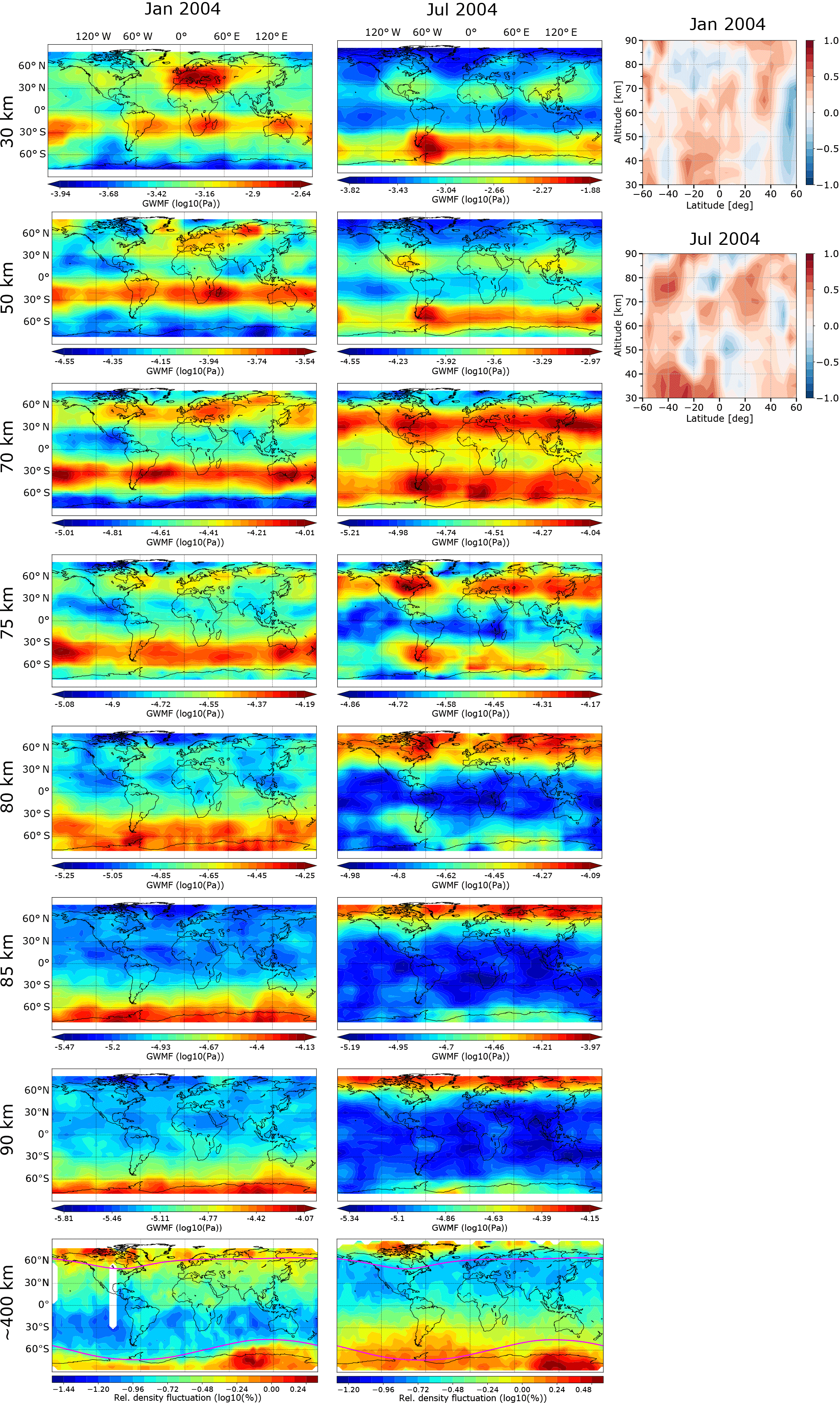
Figure 6 Global maps of GWMF derived from SABER observations (1st–7th rows, 1st two columns) and the ARDF derived from CHAMP observations (last row, 1st two columns), as well as correlation coefficients (last columns) for January and July 2004. Only data equatorward of 60^∘ magnetic latitudes (magenta lines) on CHAMP global maps are used for calculating correlations.

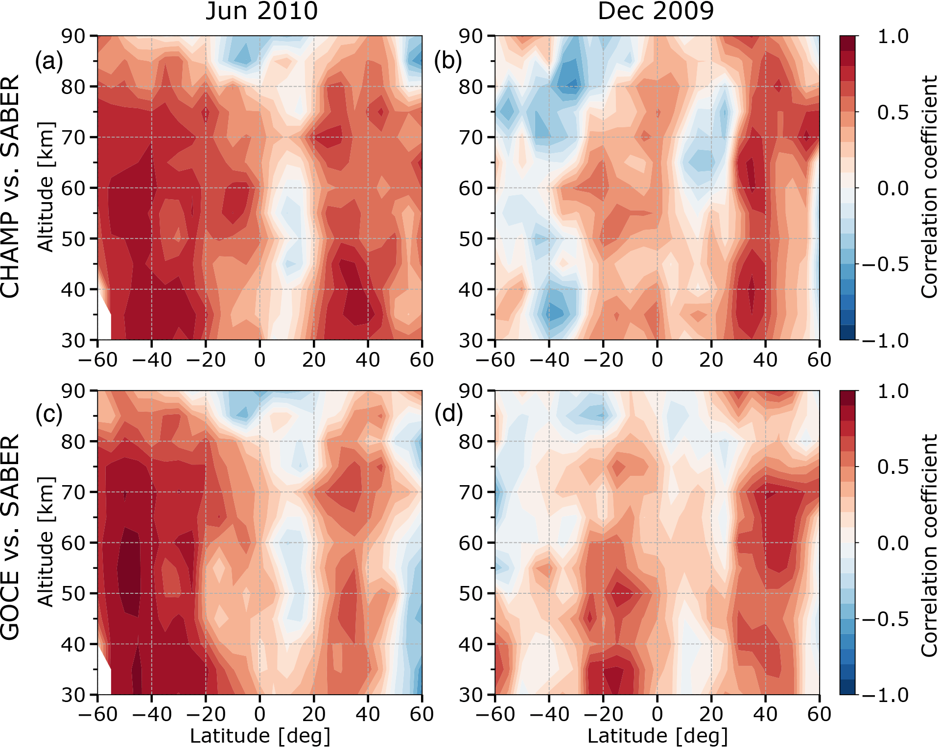
Figure 7 Correlations between (a, b) CHAMP ARDF and SABER GWMF and (c, d) GOCE ARDF and SABER GWMF for (a, c) boreal summer and (b, d) austral summer. In June 2010 (a, c) the two satellites were at almost the same altitude, while in December 2009 (b, d) CHAMP was at a higher altitude (310 km) than GOCE (270 km).

In the Southern Hemisphere (summer hemisphere), enhancements in CHAMP observations are found over continents. In particular, enhancements over South America, over the south of Africa and over Australia can be seen clearly. These locations are also hotspots of convective GWs, which can be seen from SABER observations at 30 km. This similarity explains the good correlations found in the summer subtropics in the Southern Hemisphere from 30 up to ∼60 km altitude (Fig. 6, last column, upper panel). The decrease in the correlation starting from ∼60 km altitude likely suggests the strong dissipation of primary GWs at this level.

For the boreal summer (July 2004), CHAMP ARDF at 400 km show a clear enhancement over the southern tip of the Andes and less pronounced enhancements above the polar night jet (Fig. 6, 2nd column, last row). Similar enhancements are also seen in SABER GWMF in the middle atmosphere (Fig. 6, 2nd column, 1st–7th rows). This similarity explains the rather good correlation found at mid and high latitudes in the Southern Hemisphere for July 2004 (Fig. 6, 3rd column, lower panel). In the summer hemisphere (Northern Hemisphere), some enhancements above continents are found in CHAMP observations. The maximum over North America is more pronounced than the enhancements over Europe and over East Asia. These enhancements are in the same latitude range as the latitude band of convective GW observed by SABER at 65–80 km altitudes. This explains the rather good correlation found at 65–80 km altitudes in the Northern Hemisphere for July 2004 (Fig. 6, 3rd column, lower panel).

In general, the ARDF observed by CHAMP show many similar features to the ones observed by GOCE. Accordingly, the CHAMP–SABER correlation also indicates many similarities to the GOCE–SABER correlation. However, the enhancements over midlatitudes in the summer hemisphere seem to be less pronounced in CHAMP observations than in GOCE observations. Overall, indications of vertical coupling by GWs with origins at the lower atmosphere are also visible in the CHAMP–SABER correlation.

3.3 Correlations between three data sets during the overlapping time

From March 2009 to September 2010, the CHAMP satellite and the GOCE satellite were both in operation. During this period, the two satellites were most of the time at different orbit altitudes, except at the end of CHAMP's lifetime (June–August 2010), when both of them were at almost the same altitude. It is interesting to consider the correlations between SABER observations and observations of both CHAMP and GOCE during this overlapping time. It should be noted that during this overlapping time, data are not always available for both CHAMP and GOCE. In particular, only from November 2009 to June 2010 are data available from both satellites, with gaps in January 2010 and May 2010. To consider the correlations for the boreal summer and austral summer, June 2010 and December 2009 are chosen. In December 2009, CHAMP and GOCE were at orbit altitudes of 320 and 270 km, respectively. In June 2010, the two satellites were at very similar orbit altitudes: CHAMP was at 285 km and GOCE was at 270 km.

In Fig. 7 the correlations between CHAMP ARDF and SABER GWMF are shown in the upper row, while the correlations between GOCE ARDF and SABER GWMF are shown in the lower row. The left column represents correlations for June 2010 (boreal summer) and the right column for December 2009 (austral summer).

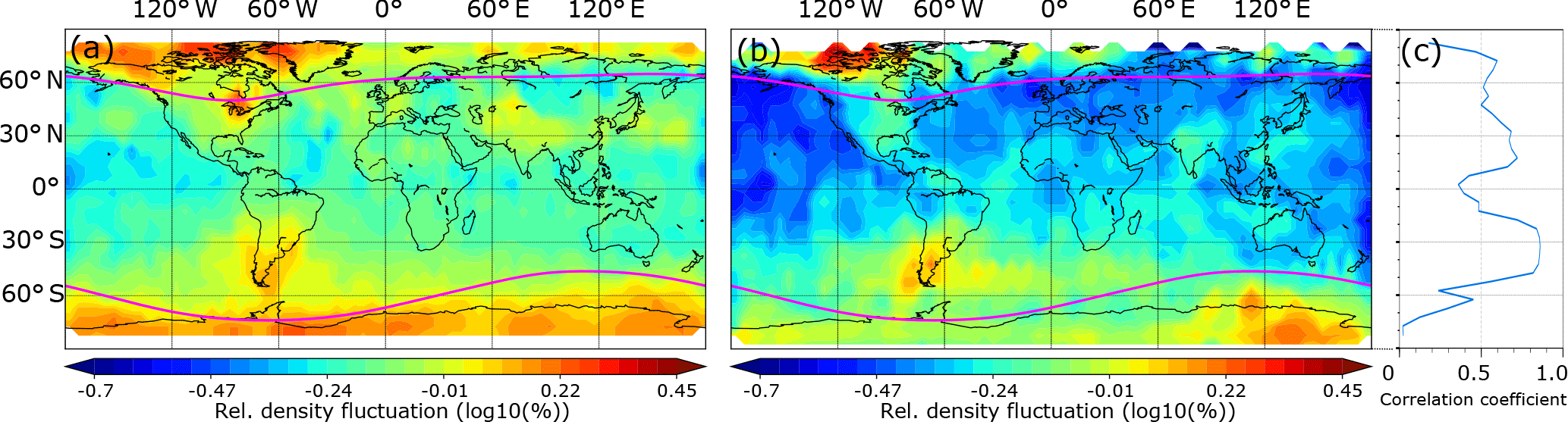
Figure 8 Horizontal distributions of ARDF for (a) GOCE satellite and (b) CHAMP satellite and (c) their spatial correlation coefficients for June 2010. Only data equatorward of 60^∘ magnetic latitudes (magenta lines) are used for calculating correlations.

First of all, similar to what we have shown in Sect. 3.1, generally positive correlations with SABER GWMF are found for both CHAMP and GOCE ARDF, for both boreal summer and austral summer. This generally positive correlation is not trivial and clearly demonstrates the vertical coupling by GWs between the middle atmosphere and thermosphere/ionosphere.

For the boreal summer, when the two satellites were at almost the same altitude, the CHAMP–SABER correlations and GOCE–SABER correlations are very similar. For example, very good correlation above the polar night jet is found, which continues up to about 85 km altitude. In the summer subtropics, good correlation is also found. The correlation here decreases first at about 60 km and then decreases again at about 80–85 km altitude. These altitudes are likely the regions where many primary convective GWs break. At low latitudes or near the Equator, both CHAMP-SABER and GOCE–SABER correlations are low or even negative. This, as we discussed above, could be related to the lack of GW patterns at low latitudes.

For the austral summer, similar features between CHAMP–SABER and GOCE–SABER correlations are also a maximum above the polar night jet and another maximum over the summer subtropics. Nevertheless, the similarity between CHAMP–SABER and GOCE–SABER correlations is weaker for the austral summer in comparison with the boreal summer. Several reasons are likely candidates for this weaker similarity. Very likely reasons are the difference in observation geometry, differences in the convective GW spectrum between the Northern Hemisphere and Southern Hemisphere (e.g., Ern and Preusse, 2012; Trinh et al., 2016) as well as the more complex terrain in the Northern Hemisphere, which leads to a less stable polar vortex. Another possible reason is the larger difference in orbit altitudes.

Similarities between CHAMP–SABER and GOCE–SABER correlations in December 2009 seem to indicate that many GWs observed at CHAMP orbit altitude (320 km) and at GOCE orbit altitude (270 km) have the same origins. In other words, they both likely have an intimate correlation with the GW distributions in the middle atmosphere, which are observed by the SABER instrument.

To further look at the time period when the two satellites are at almost the same orbit altitude, we show in Fig. 8 the horizontal distributions of GOCE ARDF (Fig. 8a) and CHAMP ARDF (Fig. 8b) for June 2010. Both panel (a) and panel (b) are plotted using the same color scale. As Fig. 8 shows, GOCE distribution and CHAMP distribution are generally very similar in both magnitude and structure. In particular, maxima over the southern tip of America, North America, India, and East Asia show up in both GOCE and CHAMP observations. Further, panel (c) shows that positive correlations are found at all latitudes. In the considered latitude range of [60^∘ S, 60^∘ N], correlation coefficients are mostly above 0.5. Nevertheless, some differences exist. One of the clear differences is that the enhancement over Great Lakes in North America is observed by GOCE but does not show up clearly in CHAMP data. GWs are highly intermittency and localized. Further, GOCE data and CHAMP data are both in situ. Thus, one satellite might see an significant wave event while the other satellite missed it. This, in addition to the differences in observation geometry and local time, may be the reason for the difference over Great Lakes.

The good agreement between CHAMP and GOCE observations is not self-evident, keeping in mind that the density determination algorithm is different for CHAMP and GOCE (for GOCE, the ion thruster data had to be used). This good agreement is therefore an overall validation of the analysis method.

The shape of GW distributions at high altitudes can be significantly influenced by solar activity. Long-term observations of the CHAMP satellite offer an opportunity to study the variation of CHAMP–SABER correlation with respect to solar activity. We performed this investigation using the 10.7 cm solar radio flux as an indicator of solar activity. However, we did not find any clear connection between CHAMP–SABER correlation and solar activity during the period from 2002 to 2010 (not shown).

4 Summary and discussion

In this study we investigated the vertical coupling by gravity waves between the middle atmosphere and the upper atmosphere (thermosphere/ionosphere). In the middle atmosphere, GW activity is presented by absolute GWMF derived from temperature measurements of the SABER instrument. In the upper atmosphere, the parameter presenting GW activity is the ARDF. To calculate these ARDF, the mass densities from two satellite missions, GOCE (at ∼250 km altitude) and CHAMP (at ∼400 km altitude), are used. In order to investigate the vertical coupling, we analyzed both global distributions as well as correlation coefficients along the longitude direction. The main findings can be summarized as follows.

1. For the boreal summer and austral summertime, when GW sources in the lower atmosphere are most active, positive correlations are generally found. This is not self-evident and clearly shows that there is a link between the GW distributions in the middle atmosphere and thermosphere/ionosphere. In other words, this clearly indicates the vertical coupling by GWs between the middle atmosphere and the thermosphere/ionosphere. In particular, the fact that good spatial correlations are found with the gravity wave distribution at altitudes as low as 30 km indicates that the distribution of gravity wave sources in the troposphere and lower stratosphere is still important in the T/I. There exist previous GCM studies, which have shown direct GW penetration into the thermosphere. For example, Yiğit et al. (2009) and Yiğit and Medvedev (2009) have demonstrated the global importance of GWs of lower atmospheric origin in the energy and momentum budget of the thermosphere. There are also other model studies, which suggest that breaking of primary GWs can generate secondary GWs and these secondary GWs in turn can propagate up to the thermosphere (e.g., Zhou et al., 2002; Vadas and Liu, 2009, 2013; Vadas and Crowley, 2010; Vadas, 2013; Vadas et al., 2014).

2. Good correlations are very often found over the winter polar vortex and over the summer midlatitudes. While the good correlations above the winter polar vortex likely indicate the propagation of mountain waves and GWs generated by unbalanced jet streams up to the thermosphere, the consistency between SABER and GOCE, CHAMP horizontal distributions as well as the positive correlations between them above the summer midlatitudes indicate quite clearly the propagation of convective GWs up to the thermosphere. This evidence of propagation of convective GWs is a new finding and complementary to previous studies. For example, Forbes et al. (2016) found the enhancements of density fluctuations over the southern tip of the Andes, which are likely related to mountain waves, but they did not find similar evidence for convective GWs. In another study, Park et al. (2014) also found the same mountain wave hotspot in CHAMP mass density. However, clear evidence for convective GWs could not be confirmed.

3. At high altitudes, SABER global distributions are much more uniform than distributions at lower altitude. Apart from the high values of GWMF in the cold summer mesopause, no particular strong hotspots of GWs can be noticed. This is likely caused by GW dissipation. At altitudes where SABER distributions becomes more uniform, the correlation with GOCE and CHAMP observations sometimes drops. The altitude where the correlation drops changes from year to year and from latitude to latitude, but very often is found between 60 and 80 km. At these altitudes, where strong decreases in correlation are found, it is expected that many “primary” GWs will break. Above this breaking level, surviving primary GWs or possibly generated secondary GWs or both of them will further propagate up to the thermosphere.

4. Above the polar night jet, the altitude where correlation drops seems to be related to the top of the polar vortex. Therefore, this altitude of drop should also be impacted by SSW events. A study dedicated to the effect of SSWs, however, would require observations of higher time resolution than the monthly average.

5. In February 2011, we found an equatorial structure in the GW distribution that is likely related to atmospheric tides. This type of triple or quadruple structure is often seen in both middle atmosphere and thermosphere/ionosphere and could be an effect of the DE3 tide which is often seen as “wave 4” in the thermosphere/ionosphere winds observed by satellite. It could also be related to GWs generated by tropical deep convection. This topic, however, is beyond the scope of the current study and also requires future investigation.

In a difference from Forbes et al. (2016) and Park et al. (2014), our study considers single-month data instead of averaged data over several years. This approach has the advantage of capturing the annual variation of GW activity and therefore is more suitable for studying vertical coupling processes. On the other hand, data from GOCE and CHAMP for 1 month sometimes have more gaps and can be more noisy than the data averaged for several years.

Our approach of calculating the correlation coefficients along the longitude direction has its limitations. As we have seen in Sect. 3, in some cases, similarities are seen quite clearly in the horizontal distributions but the correlation coefficients are not very high. This is probably due to the fact that GWs propagate horizontally and smear out while propagating upwards. This will create the shifts in both longitude and latitude directions of the same GWs between different altitude levels.

The horizontal wavelength considered in our study in the T/I ranges from about 160 to about 650 km. The lower limit is similar to the lower limit of SABER but our SABER data contain also horizontal wavelengths much longer than the 650 km limit. It should be noticed, however, that we here use GWMF. This quantity emphasizes shorter horizontal wavelengths. As an additional cross check, the SABER data were filtered for horizontal wavelengths <1000 km, and the calculation of correlations was repeated (not shown). This cross check, however, did not reveal significant differences to the shown results.

By looking only at the observations, two questions arise: (1) are there primary GWs from lower altitudes which propagate all the way up and carry the imprint of the GW distributions from lower altitudes, and are these waves just not seen in the altitude range of 75–90 km due to an overall background? (2) Is the distribution of secondary GWs, which is caused by the dissipation of GW hotspots, not as uniform as seems? This non-uniformity of the secondary GWs might just not show up at 80–90 km, but re-emerges at higher altitudes when these structures become visible again due to amplitude growth. To answer these questions, a combination of observational studies with model studies of propagation of GWs, which can cover the altitude range from 30 up to ∼400 km, is important and can provide significant insights into vertical coupling processes. Modeling studies of GW propagation into the thermosphere have been conducted. Different propagation mechanisms including direct propagation (e.g., Yiğit et al., 2009; Yiğit and Medvedev, 2010; Yiğit et al., 2012) as well as propagation with generation of secondary GWs (e.g., Miyoshi and Fujiwara, 2008; Vadas and Liu, 2009, 2013; Vadas and Crowley, 2010; Vadas, 2013; Vadas et al., 2014) have been investigated. Further studies should be performed and possibly be expanded in the context of recent observations.

In spite of these limitations, the current study clearly indicates that there is vertical coupling by GWs between the middle atmosphere and the thermosphere/ionosphere. In particular, clear evidence of propagation of convective GWs up to the thermosphere/ionosphere is found. This study can be a helpful guidance for model studies of GW propagation, which covers a wide altitude range from 30 to about 400 km.