the Creative Commons Attribution 4.0 License.
the Creative Commons Attribution 4.0 License.
 | 16 Mar 2018
Variability and trend in ozone over the southern tropics and subtropics
Abdoulwahab Mohamed Toihir
Thierry Portafaix
Venkataraman Sivakumar
Hassan Bencherif
Andréa Pazmiño
Nelson Bègue
Long-term variability in ozone trends was assessed over eight Southern Hemisphere tropical and subtropical sites (Natal, Nairobi, Ascension Island, Java, Samoa, Fiji, Reunion and Irene), using total column ozone data (TCO) and vertical ozone profiles (altitude range 15–30 km) recorded during the period January 1998–December 2012. The TCO datasets were constructed by combination of satellite data (OMI and TOMS) and ground-based observations recorded using Dobson and SAOZ spectrometers. Vertical ozone profiles were obtained from balloon-sonde experiments which were operated within the framework of the SHADOZ network. The analysis in this study was performed using the Trend-Run model. This is a multivariate regression model based on the principle of separating the variations of ozone time series into a sum of several forcings (annual and semi-annual oscillations, QBO (Quasi-Biennial Oscillation), ENSO, 11-year solar cycle) that account for most of its variability.
The trend value is calculated based on the slope of a normalized linear function which is one of the forcing parameters included in the model. Three regions were defined as follows: equatorial (0–10∘ S), tropical (10–20∘ S) and subtropical (20–30∘ S). Results obtained indicate that ozone variability is dominated by seasonal and quasi-biennial oscillations. The ENSO contribution is observed to be significant in the tropical lower stratosphere and especially over the Pacific sites (Samoa and Java). The annual cycle of ozone is observed to be the most dominant mode of variability for all the sites and presents a meridional signature with a maximum over the subtropics, while semi-annual and quasi-biannual ozone modes are more apparent over the equatorial region, and their magnitude decreases southward. The ozone variation mode linked to the QBO signal is observed between altitudes of 20 and 28 km. Over the equatorial zone there is a strong signal at ∼26 km, where 58 % ±2 % of total ozone variability is explained by the effect of QBO. Annual ozone oscillations are more apparent at two different altitude ranges (below 24 km and in the 27–30 km altitude band) over the tropical and subtropical regions, while the semi-annual oscillations are more significant over the 27–30 km altitude range in the tropical and equatorial regions. The estimated trend in TCO is positive and not significant and corresponds to a variation of % decade−1 (averaged over the three regions). The trend estimated within the equatorial region (0–15∘ S) is less than 1 % per decade, while it is assessed at more than 1.5 % decade−1 for all the sites located southward of 17∘ S. With regard to the vertical distribution of trend estimates, a positive trend in ozone concentration is obtained in the 22–30 km altitude range, while a delay in ozone improvement is apparent in the UT–LS (upper troposphere–lower stratosphere) below 22 km. This is especially noticeable at approximately 19 km, where a negative value is observed in the tropical regions.
- Article
(10567 KB) - Full-text XML
- BibTeX
- EndNote


Atmospheric ozone protects all life on earth from damaging solar ultraviolet radiation. About 90 % of ozone is observed in the stratosphere where it is strongly influenced by various photochemical and dynamical processes. Three processes determine stratospheric ozone distribution and concentration, namely ozone production, destruction and transport. While ozone concentration in the upper stratosphere (35–50 km) is primary determined by the processes of photochemical creation and destruction, ozone concentration in the lower and middle stratosphere (below 30 km) is strongly affected by transport (Portafaix et al., 2003; Bencherif et al., 2007, 2011; El-Amraoui et al., 2010). Ozone is formed primarily in tropical regions as a result of a reaction between atmospheric oxygen and the ultraviolet component of incident solar radiation; it is then subsequently transported and distributed to higher latitudes following the Brewer–Dobson circulation (Weber et al., 2011). The combination of these processes contributes to the overall spatiotemporal distribution and variability of atmospheric ozone.
The variability in ozone levels also depends on several dynamic proxies and the chemical evolution of ozone-depleting substances (ODS). Since 1980, anthropogenic ODS emissions reaching the stratosphere have led to a decline in global ozone concentration (Sinnhuber et al., 2009). However, recent observations have indicated that the decreasing trend in stratospheric ozone has been halted from the mid-90s (1995–1996), and an upward trend has been observed at 60∘ N–60∘ S since 1997 (Jones et al., 2009; Nair et al., 2013; Kyrölä et al., 2013; Chehade et al., 2014; Eckert et al., 2014). This increasing trend in stratospheric ozone is associated with a decrease in atmospheric chlorine and bromine compounds as a direct result of the Montreal Protocol which regulates ODS emission (United Nation Environment Program, UNEP 2009). From the present and going forward, this increase in stratospheric ozone is expected to begin to be more widely observable on a global scale (Steinbrecht et al., 2009; WMO (World Meteorological Organization, 2010, 2014). However, Butler et al. (2016) have shown that tropical ozone will not recover to typical levels of the 1960s by the end of the 21st century. Depending on the specific processes involved, climate change can induce modifications in the stratosphere that can delay or accelerate ozone recovery. Greenhouse gas (GHG) induced stratospheric cooling should lead to increased photochemical ozone production and slower destruction rates via the Chapman cycle (Jonsson et al., 2009). Furthermore, and with direct relevance to the region under study, acceleration of the Brewer–Dobson circulation due to tropospheric warming is thought to lead to decreases/increases in tropical/middle latitude stratospheric ozone.
It is important to create a consistent and reliable dataset in order to quantify ozone variability, to estimate trends and to validate models used for predicting future evolution of ozone levels (Randel and Thompson, 2011). The work presented here investigates the period 1998–2012 where an increase in stratospheric ozone is expected to be measurable. The aim of this study is to investigate the current behaviour of seasonal and inter-annual ozone variability over the southern tropics and subtropics and to analyse whether the expected ozone recovery is effective in the selected study region and at which altitude level ozone increase is significant. The WMO (2014) reported a divergence in ozone profile trends computed from individual instruments in the lower stratospheric tropical region. Sioris et al. (2014) showed a declining ozone trend for OSIRIS data, while Gebhardt et al. (2014) reported an increasing ozone trend using measurements from the SCanning Imaging Absorption spectroMeter for Atmospheric CHartographY (SCIAMACHY) and Aura Microwave Limb Sounder (MLS) instruments. Therefore, a study of ozone levels at tropical latitudes and present in the lower and middle stratosphere is of paramount importance. The trend analysis of two types of ozone data is relevant with respect to this study, namely, total column ozone (TCO) and vertical ozone profile measurements. While the TCO analysis offers the best way to provide information on ozone variability for the complete ozone layer, profile analysis allows for the investigation of ozone behaviour at different altitude levels (Nair et al., 2013).
Ozone profile measurement is usually achieved by ground-based lidar instruments, satellite observation and ozonesondes. However, observation by ozonesonde is often preferred due to its high vertical resolution. SHADOZ (Southern Hemisphere Additional Ozonesonde) is the only network which provides ozonesonde profiles over the southern tropics and subtropics. It has a precision of approximately 5 % with a vertical resolution between 50 and 100 m (Thompson et al., 2003a). Previously radiosonde observations from SHADOZ networks have been used to validate tropospheric ozone observations obtained from satellites (Ziemke et al., 2006, 2011), to study the stratospheric altitude profile of ozone and water vapour in the Southern Hemisphere (Sivakumar et al., 2010), to investigate the dynamic characteristics of the Southern Hemisphere tropopause (Sivakumar et al., 2006, 2011; Thompson et al., 2012), to study seasonal and inter-annual variation of ozone and temperature between the atmospheric boundary layer and the middle stratosphere (Thompson et al., 2003b; Diab et al., 2004; Sivakumar et al., 2007; Bègue et al., 2010; Mze et al., 2010) and to analyse the variability and trends in ozone and temperature in the tropics (Lee et al., 2010; Randel and Thompson, 2011).
In this paper, SHADOZ profiles recorded at eight Southern Hemisphere stations were used to investigate seasonal and inter-annual variability of ozone and to estimate the trends at different stratospheric pressure levels. The TCO measurements were performed based on Dobson and SAOZ (Système d'Analyse par Observation Zénithale) ground-based instruments (Pommerau and Goutail, 1988; Dobson, 1931). However, ground-based data were only available for three of the eight stations considered in this work. Satellite observations were therefore used in order to complete ground-based observations, particularly at tropical sites (Nairobi, Java, Samoa, Fiji and Ascension Island) where ground-based datasets were incomplete or non-existent. The chosen satellite datasets are OMI (Ozone Monitoring Instrument) and TOMS (Total Ozone Mapping Spectrometer) (McPeters et al., 1998; Bhartia, 2002) because of their high-quality ozone data. The TOMS instrument has facilitated the recording of long-term ozone measurements on both global and regional scales. TOMS instruments were successfully flown aboard several satellites from 1978 to 2005, with the latest instrument aboard the Earth Probe (EP) satellite operational from July 1996 to December 2005. In the framework of the EOS (Earth Observing System) programme, TOMS was replaced by the OMI instrument launched onboard the Aura satellite (July 2004 and operational to the present). The combined TCO data recorded from ground-based instrumentation and satellites were used to investigate ozone variability and trends over the selected study region. Data analysis was conducted using a multivariate regression model known as Trend-Run (Bencherif et al., 2006; Bègue et al., 2010).
Multivariate regression models are considered powerful tools to study stratospheric ozone variability and trends (Randel and Thompson, 2011; Kyrölä et al., 2013; Nair et al., 2013; Bourassa et al., 2014; Gebhardt et al., 2014; Eckert et al., 2014). In these models, the choice of proxies is important as the indexes of these proxies are often chosen based on atmospheric forcings that have been historically accepted as having an influence on ozone variability (Damadeo et al., 2014). Butchart et al. (2003) analysed equatorial ozone variability based on a coupled stratospheric chemistry and transport model. They observed a strong QBO (Quasi-Biennial Oscillation) signal in total column ozone variability with an observed correlation between the stratospheric ozone anomaly and the westerly wind distribution higher than 50 %. Brunner et al. (2006) demonstrated the existence of a strong QBO signal in ozone variability throughout most of the lower stratosphere, with a peak amplitude in the tropics of the order of 10–20 %. The ozone–QBO relationship has been discussed in several papers, as well as ENSO (El Niño–Southern Oscillation) influence on ozone variability. ENSO events are linked to coherent variations of the ozone zonal mean in the tropical lower stratosphere, tied to fluctuations in tropical upwelling (Randel et al., 2009). Randel and Thompson (2011) observed a negative signal in ozone variability exhibited by the ENSO index with a magnitude of around 6 % in the lower stratosphere.
It is known that solar flux has also contributed to the timescale variability of ozone (Zerefos et al., 1997; Randel and Wu, 2007). Several studies have shown that when the solar activity is high, larger amounts of ozone are formed in the upper stratosphere. Maximum ozone levels should therefore occur during periods of high solar activity (Haigh, 1994; Labitzke et al., 2002; Gray et al., 2010). However, Efstathiou and Varotsos (2013) demonstrated that the effect of the solar cycle response on total column ozone was caused by dynamical changes which were related to solar activity. It has been reported by Austin et al. (2008) that the solar flux response to long-term ozone variation is around 2.5 %, with a maximum in the tropics. Soukharev and Hood (2006) have reported that the solar cycle response to ozone variability is positive and statistically significant in the lower and upper stratosphere but insignificant over the middle stratosphere. In this investigation, QBO, ENSO and solar flux proxies were used as inputs in the Trend-Run model to simulate inter-annual ozone variation over the selected study region. Annual and semi-annual cycles were taken into account in order to quantify their impact on seasonal and annual variability.
This paper is organized as follows: Sect. 2 describes data and instrumentation used in this investigation and Sect. 3 describes the Trend-Run model and presents the method adopted for data analysis. Results detailing ozone trends and variability are presented in Sect. 4. Section 5 concludes this investigation with a summary of important results.
2.1 TCO from ground-based observations
The ground-based instruments employed in this investigation are Dobson and SAOZ spectrometers. TCO data obtained from these instruments are available from the World Ozone Ultraviolet radiation Data Centre (WOUDC, http://www.woudc.org/) and the Network for the Detection of Atmospheric Composition Change (NDACC, http://www.ndsc.ncep.noaa.gov/) websites. The Dobson spectrophotometer was the first instrument developed to measure TCO (Dobson, 1931) and the first TCO measurement was made in 1926 at Arosa, Switzerland. Dobson spectrophotometers were initially distributed at northern middle latitudes and then later moved to include observations in the Southern Hemisphere. At present, ground-based ozone measurements using Dobson spectrophotometers are widespread globally. The Dobson network currently consists of more than 80 stations, with most instruments calibrated following the standard reference D 83 which is recognized by the ESRL (Earth System Research Laboratory) and the WMO (Komhyr et al., 1993). The relative uncertainty associated with the Dobson instrument has been assessed at approximately 2 % (Basher, 1985). In this work, TCO recorded from Dobson instruments located at Natal (equatorial site: 35.38∘ W, 5.42∘ S) and Irene (subtropical site: 28.22∘ E, 25.90∘ S) was used. The measurement principle of the Dobson spectrometer is based on a UV radiation differential absorption technique in a wavelength range where ozone is strongly absorbed compared to one where ozone is weakly absorbed. Total column ozone observations are performed by measuring the relative intensities at selected pairs of ultraviolet wavelengths. The most used wavelengths are the double pair (305.5/325.5 nm and 317.6/339.8 nm) and (311.45/332.4 nm and 316.6/339.8 nm) emanating from the Sun, moon or zenith sky (WMO, 2003, 2008). For further information regarding the Dobson spectrometer functioning, the reader may refer to the studies outlined by Komhyr et al. (1989, 1993).
The SAOZ spectrometer was developed by the CNRS (Centre National de la Recherche Scientifique). In 1988, it was used for the first time at Dumont d'Urville (Antarctica) to measure stratospheric ozone during the polar winter. SAOZ is a passive remote sensing instrument operating in the visible and ultraviolet ranges. It measures the sunlight scattered from the zenith sky in the wavelength range between 300 and 600 nm. The SAOZ instrument is able to retrieve the total column of ozone and NO2 in the visible band with an average spectral resolution of around 1 nm using the differential optical absorption spectroscopy (DOAS) technique. At Reunion, a SAOZ instrument has been operational since 1993 within the framework of NDACC. SAOZ ozone measurements have been performed during sunrise and sunset with a precision of <5 % and an accuracy of <6 % (Hendrick et al., 2011). In the present work, the daily average of TCO was taken as the mean value of sunrise and sunset observations (86–91∘ SZA) recorded at Reunion. SAOZ TCO measurements have been shown to be in good agreement with OMI-TOMS (Pastel et al., 2014; Toihir et al., 2013) and Infrared Atmospheric Sounding Interferometer (IASI; Toihir et al., 2015a) measurements. Further details can be found in Pazmiño (2010).
2.2 TCO from satellite observations
Satellite data employed in this investigation were obtained from the EP-TOMS and OMI-TOMS L2 data products. The EP-TOMS data product is the most recent (1996–2005) and the duration of other important satellite observations include the TOMS instrument onboard the Nimbus-7 satellite (1978–1993), Meteor-3 (1991–1994) and ADEOS (1996–1997). On 2 July 1996, EP-TOMS was the only instrument launched onboard the Earth Probe satellite. It was launched into a polar orbit with an initial altitude of 500 km and an inclination angle of 98∘. However, after the failure of the ADEOS satellite, the EP-TOMS instrument was raised to an altitude of 739 km with an inclination angle of 98.4∘ This was done in order to provide complete global coverage of ozone and other species such as sulfur dioxide. The TOMS instrument is a downward nadir viewing spectrometer that measures both incoming solar energy and backscatter ultraviolet radiance at six different wavelengths (379.95, 359.88, 339.66, 331.06, 317.35 and 312.34 nm) with a spatial resolution of 50 km×50 km. The instrument uses a single monochromator and a scanning mirror to sample the backscattered solar ultraviolet radiation at 35 sample points at 3∘ intervals along a line perpendicular to the orbital plane (Bramstedt et al., 2003). TOMS data used in this work are an overpass product and are available online from the website link http://acdisc.gsfc.nasa.gov/opendap/EarthProbe_TOMS_Level3/contents.html. For more details on the TOMS instrument and the associated data product, the reader may refer to the EP-TOMS data product user guide document (McPeters et al., 1998).
As previously mentioned, the EP-TOMS instrument was operational from July 1996 to December 2005. TCO from TOMS was therefore combined with that from OMI recorded overpass for the eight selected investigation sites in order to produce a complete ozone dataset running to December 2012. Two OMI L2 data products are available: OMI-DOAS and OMI-TOMS. However, the OMI-TOMS L2 product was chosen for this investigation due to its good agreement with the EP-TOMS data product (Toihir et al., 2014). OMI is a compact nadir viewing instrument launched aboard the Aura satellite in July 2004 into a near-polar helio-synchronous orbit at approximately 705 km in altitude. OMI operates at a spectral resolution within 0.5 nm in three spectral regions referred to as UV-1, UV-2 and VIS. In terms of spatial coverage, its viewing angle is 57∘ under a swath width of 2600 km. The ground pixel size of each scan is 13×24 km2 in the UV-2 (310–365 nm) and visible (350–500 nm) channels, and 13 km×48 km for the UV-1 (270–310 nm) channel. OMI data used in this work are overpass L2 products and are accessible from http://avdc.gsfc.nasa.gov/pub/data/satellite/Aura/OMI/V03/L2OVP/. OMI-TOMS ozone data are retrieved based on two wavelengths (317.5 and 331.2 nm are applicable under most conditions, while 331.2 and 360 nm are used for conditions of high ozone concentration and high solar zenith angle). The L2 product has a precision of ∼3 % and has shown good agreement with Dobson and SAOZ measurements over the southern tropics and subtropics (Toihir et al., 2013, 2015a). Further details relating to the OMI instrument and mode of operation can be found in the OMI Algorithm Theoretical Basis Document Volume II (Bhartia, 2002).
2.3 Ozone profiles from the SHADOZ network
Balloon-borne electrochemical concentration cell (ECC) ozonesonde devices were used to provide profile ozone measurements over the eight stations (Nairobi, Ascension Island, Java, Samoa, Fiji, Natal, Reunion and Irene) investigated in this work. These stations form part of the SHADOZ network. The geographical location of each site is illustrated in Fig. 1, while geographical coordinates and altitude a.s.l. are given in Table 1. Equipped with radiosondes for temperature, humidity and pressure measurements, the ECC ozonesonde provides vertical profiles with a resolution between 50 and 100 m from ground to the altitude where balloon burst occurs (∼26–32 km). The precisions of SHADOZ measurements have been evaluated to be ∼5 % (Thompson et al., 2003b). Further details on ECC ozonesonde instrument validation, operating mode and algorithm used for ozone partial pressure (in mPa) retrieval in each of the SHADOZ stations can be obtained from Thompson et al. (2003a, 2007) and Smit et al. (2007). In this work, analysis of vertical ozone variability was performed using SHADOZ profiles recorded over 15 years (1998–2012). These data are available from http://croc.gsfc.nasa.gov/shadoz/. The frequency of SHADOZ observations is between one and six balloon launches per month. The monthly mean profiles for a given station were taken as the average of recorded profiles during the month for that station.
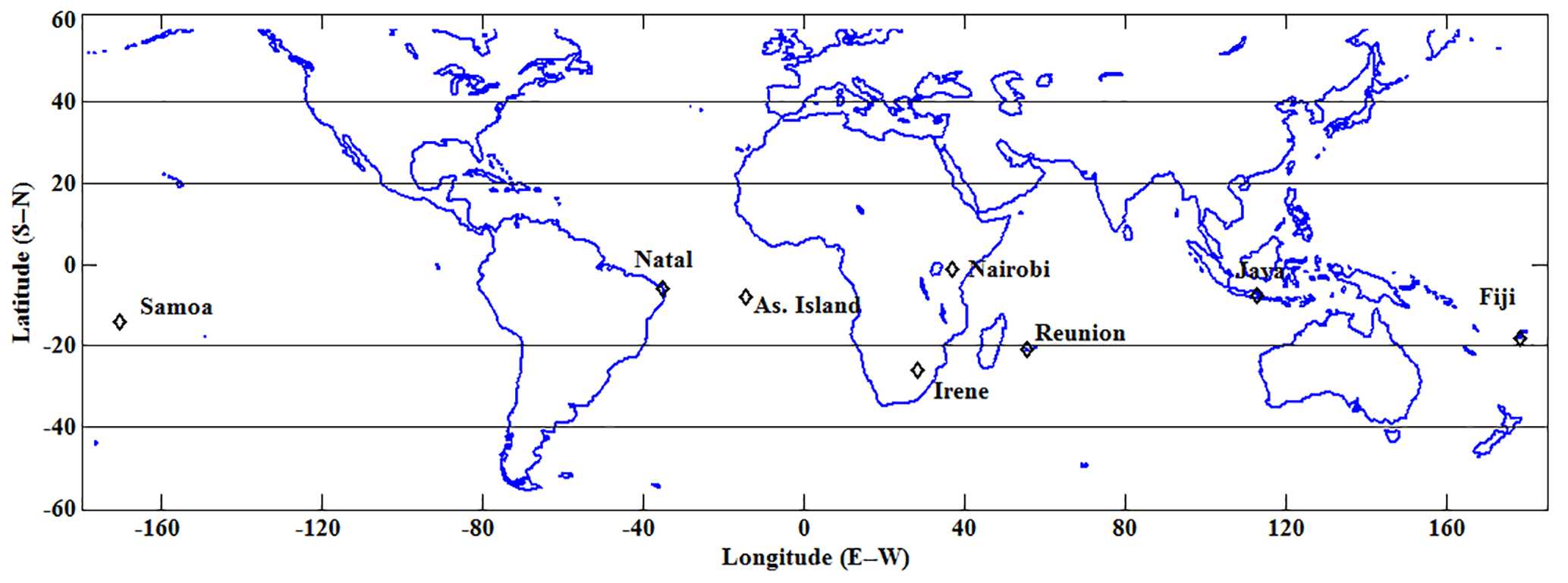
Table 1Geolocation and mean sea level (MSL) of stations investigated in this study.
3.1 Methodology
Prior to analysis of TCO variability and trends, preliminary work was completed in order to create a reliable ozone dataset for each station by merging different available measurements. The first combination exercise was performed on satellite data (TCO form OMI and TOMS) by using the monthly values of ozone recorded during the overlap observation period of the two satellites (October 2004–December 2005). The relative difference (RD) between TOMS and OMI with respect to OMI observation was calculated for individual sites as follows:
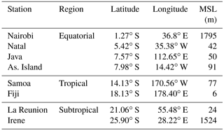
where “m” is the month in which both OMI and TOMS observations were performed. After assessing the relative difference, the bias and root mean square (rms) associated with the difference were calculated. For further details outlining the method used to calculate bias and rms, see Toihir et al. (2015a), Toihir et al. (2015b) and Anton et al. (2011). The results obtained for each individual site are presented in Table 2. The recorded biases between TOMS and OMI are positive, thereby indicating an overestimation of TOMS total column ozone with respect to OMI. However, the bias is less than 2.5 % and correlation coefficients (C) between OMI and TOMS are higher than 0.9 (see column 4 of Table 2); it is therefore reasonable to combine the two observations. As OMI measurements recorded during the study period for the chosen sites show better agreement with ground-based (Dobson and SAOZ) measurements than TOMS (see Toihir, 2016, chapter 2), the combination of OMI and TOMS was performed using the OMI observations as a reference. The data combination follows two steps: the first step consists of adjusting the TOMS dataset (January 1998 to December 2005) with respect to OMI by using the obtained rms. The absolute rms is considered the mean systematic error in Dobson units between TOMS and OMI. As TOMS ozone values are always higher than OMI values, TOMS time series (1996–2005) can be adjusted to OMI measurements as follows:
The second step is to average the measurements from OMI with the adjusted TOMS measurements recorded during the overlap observation period of the two satellites.
Table 2The computed bias, rms (root mean square) and correlation coefficient C observed between OMI and TOMS for individual stations during the period from August 2004 to December 2006.
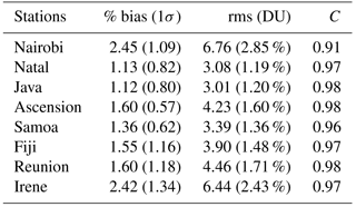
Figure 2 presents the time evolution of monthly mean TCO measurements over Reunion. Blue and black curves represent TOMS and OMI data respectively. Figure 2 highlights the existing good agreement between both TOMS and OMI observations, with similar results being reported in Toihir et al. (2014). The merged satellite time-evolution data are shown as a dotted red line in Fig. 2. The combination of the above satellite data is performed for each site under study by using the rms obtained for the site (see Table 2).
Figure 2Monthly mean of TCO as measured by TOMS (blue) and OMI (black) over Reunion. The combined measurements of OMI and TOMS data are indicated by the dashed red line.
A second method to validate this data combination consisted of a comparison of satellite data with available ground-based measurements. TCO from ground-based instruments were available at Natal, Reunion and Irene stations and ground-based and TOMS adjusted-OMI time evolutions of the TCO monthly mean over these stations are shown in Fig. 3. Figure 3 illustrates the fact that satellite data show good agreement with ground-based observation before and after the simultaneous period of TOMS and OMI observations, thereby indicating a good agreement between the merged satellite and ground-based data. Correlation coefficients C between the merged satellite measurements and ground-based data are 0.88, 0.90 and 0.97 over Natal, Irene and Reunion respectively. The obtained relative bias between satellite and ground-based observation with respect to the ground-based observation is assessed to be less than 2.5 % for individual sites. Due to this consistency existing between merged satellite data and ground-based measurements, the study of TCO variability and trends was performed using the merged satellite data for sites where no ground-based measurements existed. In the case of three stations where ground-based measurements were available, satellite and ground-based measurements were merged by adjusting the satellite dataset with respect to ground-based data.
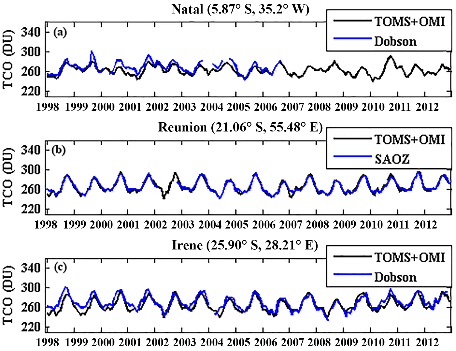
Figure 3Temporal evolution of TCO from ground-based spectrometers (blue) compared with that obtained by a combination of TOMS and OMI TCO overpass over Natal (a), Reunion (b) and Irene (c) for the period January 1998 to December 2012.
The study of vertical ozone variability and associated trends was performed based on SHADOZ ozone profile data available for the eight selected sites. In this work, 3431 profiles were examined. The number of examined profiles and the temporal coverage of data recorded for individual stations are presented in Table 3. Although the eight SHADOZ stations started measurements in 1998, the temporal coverage of the data recorded and the number of observations at each station differ. For example, observations at Ascension Island were discontinued in 2010, while no data were available in Natal during 2012. Irene SHADOZ observations were discontinued in 2006 and restarted in November 2012. Considering the discontinuity in observations and the limited number of monthly profiles, monthly data for stations with the same climatological behaviour were averaged (Mzé et al., 2010). Stations were classified into three groups based on low variability in zonal ozone distribution, the proximity of stations and the dynamical structure of the stratosphere (Ziemke et al., 2010). These groupings were near-equatorial (Nairobi, Natal, Java and Ascension Island), tropical (Samoa and Fiji) and subtropical (Reunion and Irene) and corresponded to stations located between latitude bands 0–10∘ S, 10–20∘ S and 20–30∘ S respectively. Geographical coordinates of stations are given in Table 1. Monthly profiles recorded from stations located in the same altitude band were averaged to represent the monthly mean for the selected altitude range. Figure 4 shows the time and height evolution of the constructed monthly mean ozone profile. The top (a), middle (b) and bottom (c) panels represent the monthly vertical distribution of ozone concentration between 15 and 30 km over the equatorial, tropical and subtropical regions respectively. In order to follow a more uniform data processing approach, monthly TCO values for stations from the same latitude range were averaged for specific cases. The constructed TCO time series from the procedure defined above are shown by the blue line in Fig. 5.
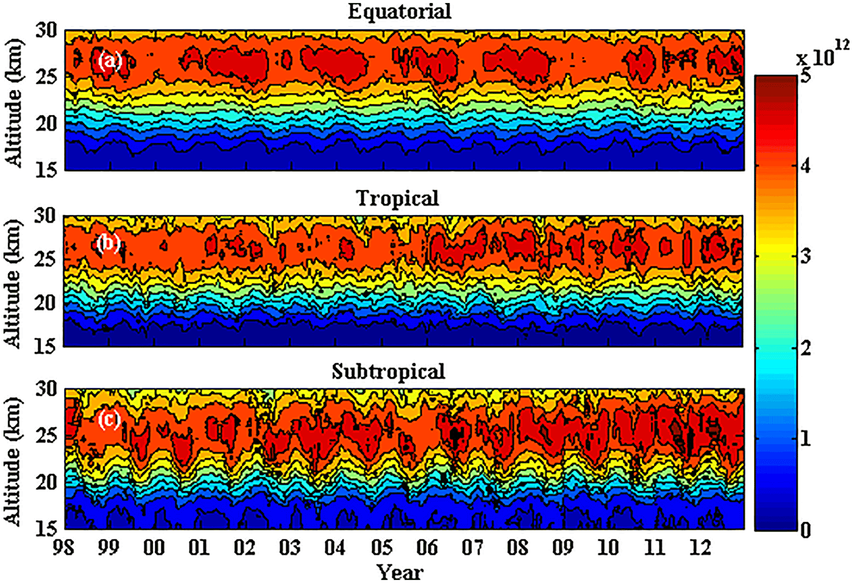
Figure 4Time–height section of ozone concentration (mol cm−3) obtained by mean monthly profiles recorded over stations located in the equatorial (a), tropical (b) and subtropical (c) regions from January 1998 to December 2012.
Table 3Time period and total number of height profiles used in this analysis for selected stations.
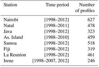
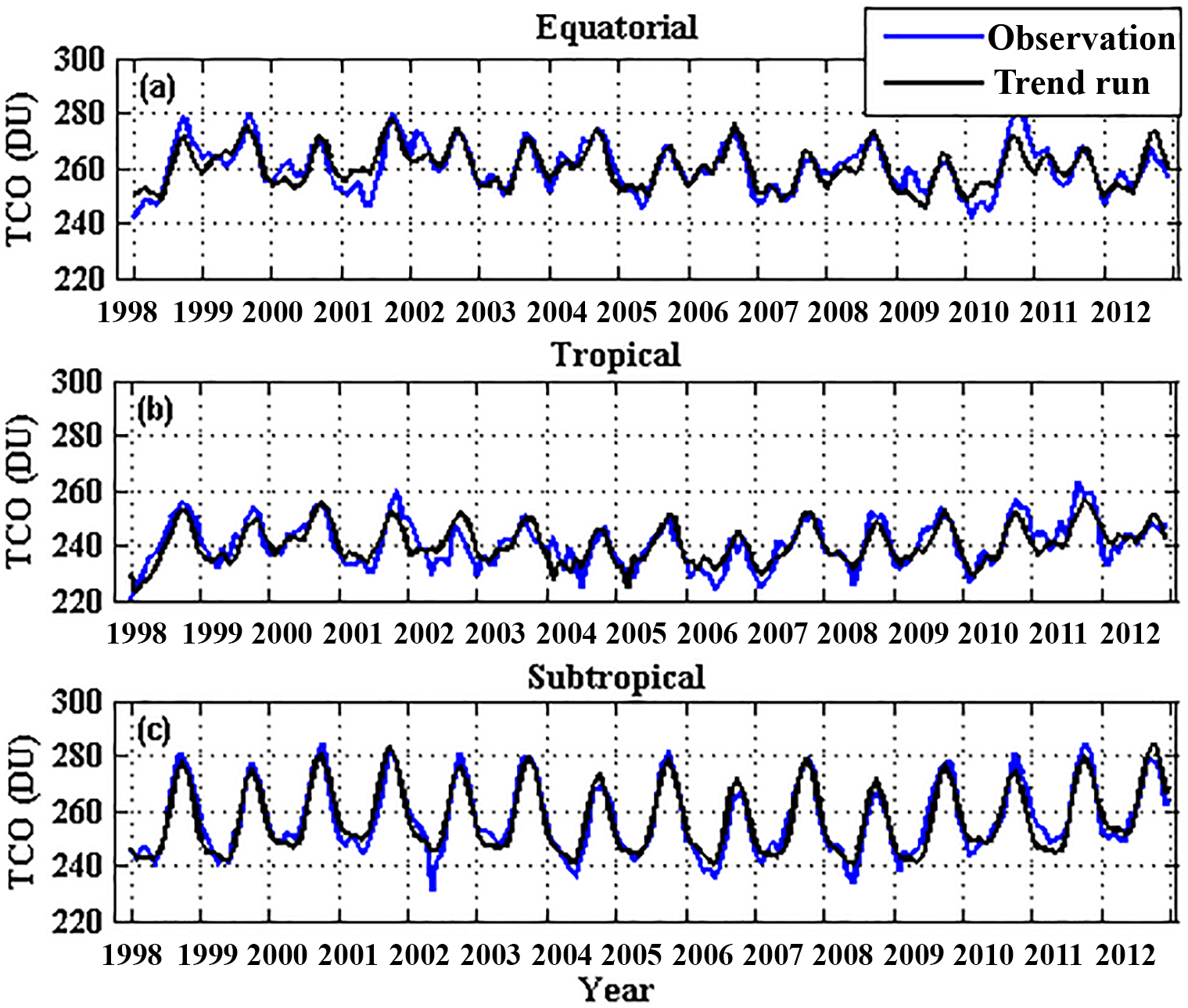
Figure 5Time evolution of monthly mean total ozone values (blue) over the equatorial (a), tropical (b) and (c) subtropical regions. The black lines represent TCO values as calculated by the Trend-Run model.
3.2 Description of the Trend-Run model
Trend-Run is a multi-regression model adapted by Reunion University and dedicated to the study of ozone and temperature variability and associated trends (Bencherif et al., 2006; Bègue et al., 2010; Toihir et al., 2014). Input parameters include monthly mean ozone values (in DU for TCO or concentration at a given pressure for high-altitude profiles) and variables that represent a significant contribution to stratospheric ozone variability. Considering the selected region (0–30∘ S) and the temporal coverage defined in this work (1998–2012), and in order to simplify analysis and interpretation of results, the parameters included in this analysis were QBO, ENSO and solar flux. Note that aerosols constitute a source of uncertainty that may affect TCO variability, notably following a major event such as a volcanic eruption. However, by using the Trend-Run model, Bencherif et al. (2006) and Bègue et al. (2010) showed that volcanic aerosol forcing from the Pinatubo eruption was weak and could be assumed negligible beyond 1996. Aerosol index is therefore not included in the framework of this present study as the ozone time series starts in 1998, 2–3 years after the post-Pinatubo eruption period. In trend calculations, a long-term linear function is generated by the model to characterize the trend index which is used among the model parameters. The trend value is calculated based on the slope of the normalized linear function. As ozone variability is also affected by annual and semi-annual oscillations (AO and SAO), these two parameters were taken into account in terms of model inputs. They may be described by a sinusoidal function as shown below:
where “m” is the monthly temporal parameter and .
I is a phasing coefficient between the temporal signal of ozone and the sinusoidal annual or semi-annual function. The ENSO parameter is based on the Multivariate ENSO Index (MEI), while the solar cycle is the solar 10.7 cm radio flux. These two parameters were obtained from the NCEP/NCAR website: http://www.esrl.noaa.gov/psd/data/climateindices/list/. The MEI is defined by positive values during El Niño and negative values for the duration of La Niña. The chosen QBO index is the time series of zonal wind at 30 hPa over Singapore and is available from the following link: http://www.cpc.ncep.noaa.gov/data/indices/qbo.u30.index. ENSO and QBO parameters are phased with respect to ozone time series based on phasing time which define the temporal point where the variable response to ozone is maximum. The index time series of the considered parameters are first normalized and filtered to remove a possible 3-month response. The output geophysical signal Y(z,m) of ozone for a given altitude “z” is modelled as follows:
where C(z)(1–7) are regression coefficients representing the weighting of parameterized variables on geophysical signal Y and ε(z,m) is the residual term representing a noise and/or contribution of parameters not included in the model. The regression coefficients are determined based on the least-squares method in order to minimize the sum of the residual squares. It is worth noting that the degree of data independency is assessed through the autocorrelation coefficient φ of the residual term (Bencherif et al., 2006). More details on how φ is calculated for ozone data are found in Portafaix (2003). The uncertainties in coefficient C(z)(1–7) are assessed by taking into account the autocorrelation coefficient and are formulated as follows:
where and v(k) represent the variance of the residual term and the covariance matrix of the different proxies input in the linear multi-regression model respectively. Equation (5) is used to estimate error associated with trend estimation.
The temporal function is defined as the factorized signal of input proxy “P”, and is the corresponding SD (Brunner et al., 2006). The contribution of a given parameter to the total variation of inter-annual data is the ratio of a factorized signal sum of squares to the total sum of squares of the inter-annual ozone data. The amplitude of the response of the parameterized parameter (in percentage by unit of the parameter) with respect to the total variance of ozone time series is assessed based on the corresponding regression coefficient. It may be expressed as follows:
A is positive when the temporal signal of the parameter is in phase with the ozone time series, and it is negative in the opposite case.
In this investigation, ozone inter-annual variability and trends were studied using the Trend-Run model as described above. The contribution and response of dynamical forcings to TCO variability are presented and discussed in Sect. 4.2. The aim of this study was to analyse the behaviour of each individual forcing contribution and to quantify the effect of its contribution on ozone variability in terms of TCO and mixing ratio profiles for the 15–30 km altitude range. The observed solar flux response to ozone over the selected altitude range is very weak (less than 1 %); the solar flux contribution to ozone vertical distribution is therefore not discussed. Ozone trends (for the observation period) as estimated by the model are presented (per site) in the final subsection.
4.1 Model assessment
In order to quantify the fit of the regression model with original ozone data, a statistical coefficient R2 was used. The coefficient R2 is defined as the ratio of a regression sum of squares to the total sum of squares (Bègue et al., 2010) and it measures the proportion of the total variation in ozone as described by the model. When the regression model accounts for most of the observed variation in ozone time series, the value of R2 is close to unity. For the cases where the model shows little agreement with measured data, R2 decreases toward zero (Bègue et al., 2010; Toihir et al., 2014). Figure 5 shows the time evolution of total column ozone as simulated by the multi-regression model (black). The blue lines correspond to TCO measurements performed over the (a) equatorial, (b) tropical and (c) subtropical latitude bands. A good agreement between model and observations is apparent over the three regions and the best fit is observed for the extratropics. This is because the variability is usually influenced by the seasonal cycle which is well accounted for by the regression model (Eq. 3). The values obtained for the statistical coefficient R2 were 0.75, 0.71 and 0.91 for the equatorial, tropical and subtropical bands respectively. These results indicate that the model describes approximately 75, 71 and 91 % of TCO variability. This implies that the sum of the contributions of the annual cycle, semi-annual cycle, QBO, ENSO, solar flux and trend to TCO variability reached 75, 71 and 91 % for the equatorial, tropical and subtropical bands respectively. That represents how the model is able to reproduce most of the variability of the studied ozone time series. Statistical coefficients (R2) higher than 0.82 were highlighted by Toihir et al. (2014) over sites located at 30–40∘ S, while Bencherif et al. (2006) and Bègue et al. (2010) demonstrated that the Trend-Run model is able to describe approximately 80 % of the temperature variability observed over Durban (South Africa) and Reunion.
Regarding vertical ozone distribution, profiles plotted in Fig. 4 were interpolated at a vertical resolution of 0.1 km which resulted in 150 altitude levels for the range between 15 and 30 km. The multi-regression model calculation was performed for each altitude level and profiles of the coefficient of determination R2 obtained at (a) equatorial, (b) tropical and (c) subtropical bands are shown in Fig. 6. The calculated R2 values were higher than 0.6, and this indicates that the input parameters account for more than 60 % of ozone variability in the 15–30 km altitude range.
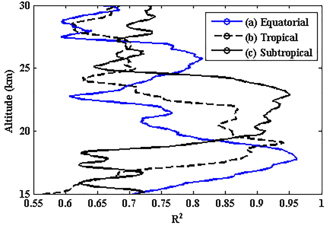
Figure 6Vertical profiles of R2 (determination coefficient) calculated by the Trend-Run model for the selected latitude range: (a) equatorial, (b) tropical and (c) subtropical regions.
A study by Brunner et al. (2006) demonstrated that high values of R2 characterized a regime dominated by seasonal variability, while R2 values between 0.3 and 0.7 described cases where ozone variability was dominated by QBO. This is in agreement with results from the present study and confirms the capacity of the Trend-Run model to retrieve consistent ozone time series. As seen from Fig. 6, values of R2 greater than 0.8 were recorded at different altitude layers depending on the region, namely, in the 16.3–26.0 km range for the equatorial region, in the 17.3–22.2 km layer for the tropics and between 18.9 and 24.5 km for the extratropics. Furthermore, this analysis demonstrates that the noted altitude ranges are dominated by a seasonal variability which is expressed by an annual cycle function in the model.
4.2 TCO variability
4.2.1 Seasonal variability
Figure 7 illustrates ozone climatology obtained by compilation of 15 years of data recorded between January 1998 and December 2012. Three regions are explored: (a) equatorial, (b) tropical and (c) subtropical. Over these selected regions, total ozone exhibited high values from July to November. A positive gradient was observed from May to the maximum annual peak in September (equatorial region) but occurred a month later in October for tropical and near-subtropical regions. The recorded positive gradient over the subtropics was the largest and this indicated a high seasonal variability in this region compared to tropical and equatorial zones. Low ozone levels were recorded during the austral summer/autumn period over the three regions. Ozone recorded in the equatorial region was high in March, April and May compared to the tropics. Two peaks were clearly observed for the equatorial region, and these highlight a semi-annual cycle with a maximum in September–October and a second maximum in March–May.
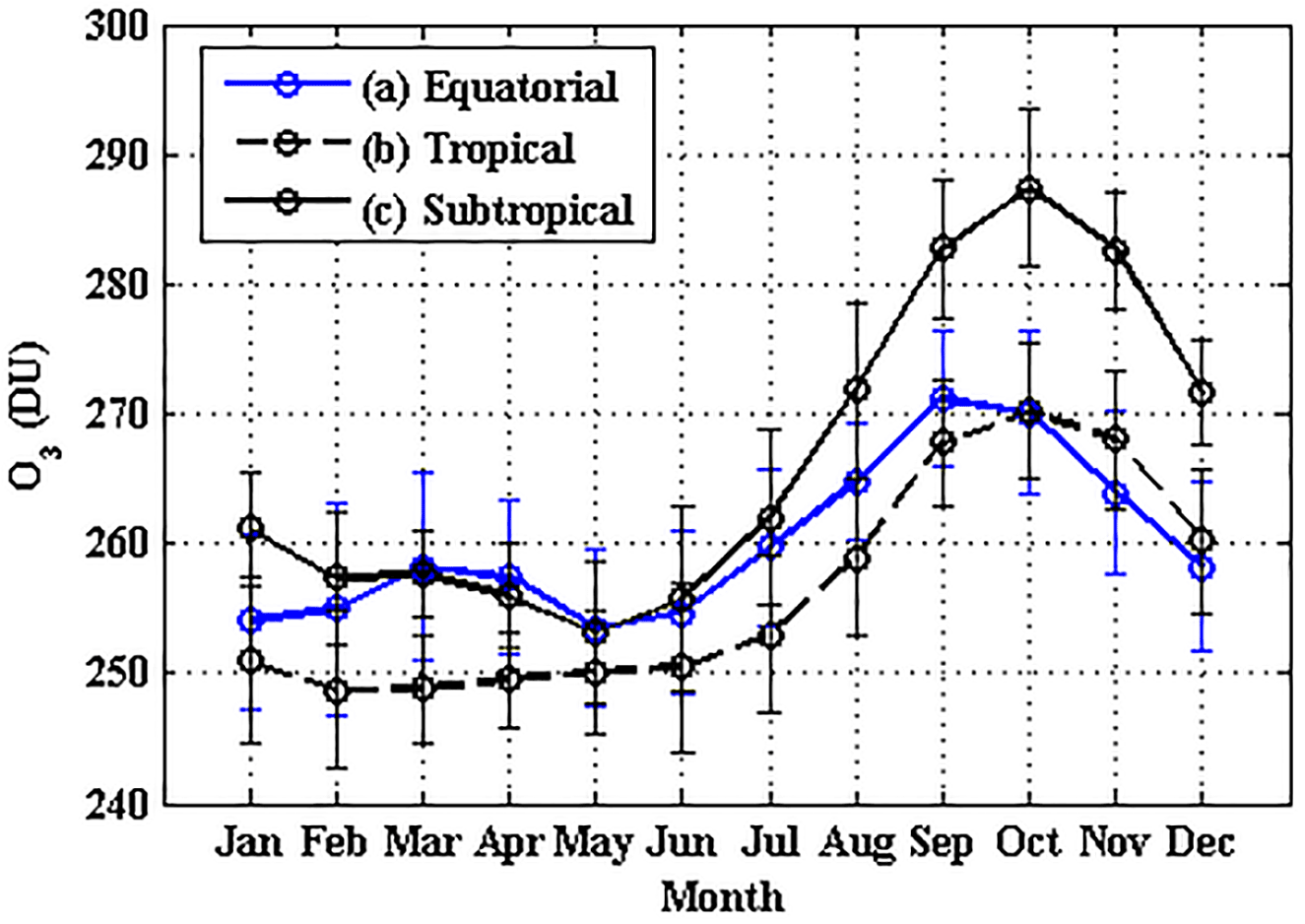
Figure 7Seasonal variations of total ozone over three different regions: equatorial (a), tropical (b) and subtropical (c) regions. Error bars represent ±1σ.
These results can be explained as follows: stratospheric ozone is formed through a photochemical reaction (Chapman, 1930) that requires a sufficient quantity of solar radiation. The equatorial region is therefore the primary site of ozone production (Coe and Webb, 2003). During the period close to equinox, solar radiation leads to an increase in ozone production over the equatorial region. During summer, ozone transport consists primarily of vertical upwelling movements which are confined to the low-latitude region. This results in less ozone being distributed to the subtropics. This effect is the main contributing factor to why a total ozone peak is observed in autumn over the equatorial region (Mzé et al., 2010). However, the semi-annual equinox process may not be the sole explanation for the maximum value recorded in the equatorial region during September spring equinox, because it is generalized over the three regions. High ozone levels recorded in winter/spring are due to transport and accumulation of ozone in the Southern Hemisphere as a result of Brewer–Dobson circulation on a regional (air mass transport from the tropics to subtropics) and global scale (from summer hemisphere to winter hemisphere) (Holton et al., 1995; Fioletov, 2008). Transport of ozone from the tropical to extratropical regions is the most dominant process during the winter period (Portafaix, 2003) and constitutes the principal reason for the observed annual maximum over the region 20–30∘ S. The decline of ozone levels during late spring and summer is explained by a decrease in ozone transport coupled with ozone photochemical loss (Fioletov, 2008). However, the observation of maximum ozone in September over the equatorial region but 1 month later over the subtropics may be explained by a delay of ozone transport between the two regions. As shown in Fig. 7, the curve of the seasonal distribution of TCO attributed to (b) the tropical region is below that of (a) the equatorial zone from January to September. While considering the process of formation and transport of ozone as described above, TCO annual records in tropical regions should be higher than that recorded over equatorial regions. However, it is important to note that both sites (Samoa and Fiji, in the 10–20∘ latitude range) are located in the Pacific Ocean. The low TCO quantity observed in the Pacific is due to a low tropospheric ozone levels over the region as a result of a zonal Wave-One observed on tropical tropospheric ozone (Thompson et al., 2003a and 2003b). Similar results were reported by Thompson et al. ( 2003a and 2003b) where low ozone levels over SHADOZ Pacific sites were observed with respect to African and Atlantic sites due to the zonal Wave-One.
The contribution of seasonal cycles (annual and semi-annual oscillations) to ozone variability obtained from the regression analysis is presented in the first and second columns of Table 4. The calculated values show that except for Nairobi, the annual cycle constitutes the predominant mode of ozone variability over the studied sites and its influence is strongly observed over the subtropics. The contribution of annual oscillations to ozone variability exhibits a latitudinal signature, with its minimum and maximum at equatorial and subtropical zones respectively. The percentage contribution of annual oscillations to TCO variability decreases equatorward from Irene (65.96±3.93 %) to Nairobi (20.33±1.89 %). As explained in Sect. 3, the annual cycle is modeled by a sinusoidal function with maximum and minimum in winter/spring and autumn/summer. This kind of annual variation mode characterizes the ozone climatology of southern tropics and subtropics (Toihir et al., 2013, 2015a). The response of annual oscillations to ozone variability obtained for individual sites and reported in Table 5 is positive. This indicates that the modeled annual cycle function is in phase with the original ozone data. However, the amplitude of the annual cycle on total variance of ozone over the subtropics is the highest, and this indicates that ozone variance is sensitive to annual oscillation in the subtropics compared to tropics. The amplitude was evaluated at approximately 5.6 % by unit of the standardized annual function in subtropical sites (Reunion and Irene) and varied between 1 and 3 % from Fiji towards the Equator.
Table 4Percentage of the contribution and corresponding SD of the annual cycle, semi-annual cycle, 11-year solar cycle, QBO and ENSO to total ozone variability for individual sites, as obtained by the Trend-Run regression model. The last column shows the corresponding value for the coefficient of determination R2.
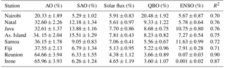
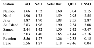
Table 5Response values of the chosen proxies (annual cycle, semi-annual cycle, solar flux, QBO and ENSO) to total ozone variability for individual sites as obtained by the Trend-Run model. The response is given in percent by unit of the normalized proxy.
Results presented in Table 4 show that on average, 13.86±1.26 % of ozone variability can be explained by semi-annual oscillations over stations located at 5–10∘ S. However, the semi-annual pattern was not apparent over Nairobi compared to the rest of the equatorial sites. The predominant mode of ozone variability in this equatorial site was the QBO (20.48±1.92 %), followed by the annual oscillations (20.33±1.89 %). The semi-annual oscillation pattern of TCO was observed to be significant at low latitude, with its maximum contribution over Ascension Island. The response values associated with semi-annual oscillation to ozone variability are presented in column 2 of Table 5 and show that a maximum in amplitude over Ascension Island was observed. Both quantities (contribution and response) decreased gradually while moving away from the Ascension Island site towards the Equator or southward. This indicates that the semi-annual oscillations of ozone are weighted at approximately 8∘ of latitude and coincide with the location where the influence of equinox processes on ozone variability is the greatest.
4.2.2 QBO contribution
The QBO constitutes the second most important parameter influencing ozone variability after seasonal oscillations. The QBO behaviour on ozone time series can be observed by removing the monthly climatological value from its monthly mean. In this investigation, the deseasonalized ozone signal was further subjected to 3-month smoothing in order to filter out smaller perturbations from intra-seasonal oscillations and to address the component due to ozone biennial oscillations.
Figure 8 illustrates the deseasonalized ozone (blue dashed curve) time series (1998–2012) for equatorial and subtropical regions. These data are superimposed with the monthly mean zonal wind data at 30 hPa over Singapore (black curve). From Fig. 8 it can be seen that the predominant variability of deseasonalized monthly ozone data is an approximately 2-year cycle linked to the QBO and represented by the zonal wind data at 30 hPa. However, the equatorial and subtropical ozone signals seem to be opposite in phase. This indicates that if an excess of ozone is recorded over the equatorial region, the subtropical zone shows a trend illustrating a deficit with respect to the monthly climatological value and vice versa. The QBO change from the Equator to the subtropics is due to a secondary circulation having an upwelling branch in the subtropics and a subsidence branch in the tropics during the westerly phase of the QBO (Chehade et al., 2014). This secondary circulation is characterized by a deceleration or an acceleration of the Brewer–Dobson circulation (BDC) during the westerly or easterly phase of the QBO respectively. The deceleration of the BDC leads to an increase in ozone in the tropics, while the acceleration leads to a decrease in ozone in the tropics. Due to this circulation, the deseasonalized TCO data over the equatorial region are in phase with the QBO index. Positive ozone anomalies correspond to the QBO westerly phase and negative anomalies are linked to the QBO easterly phase. Similar results have been determined in previous studies (Randel and Wu, 2007; Butchart et al., 2003; Zou et al., 2000; Bourassa et al., 2014; Peres et al., 2017).
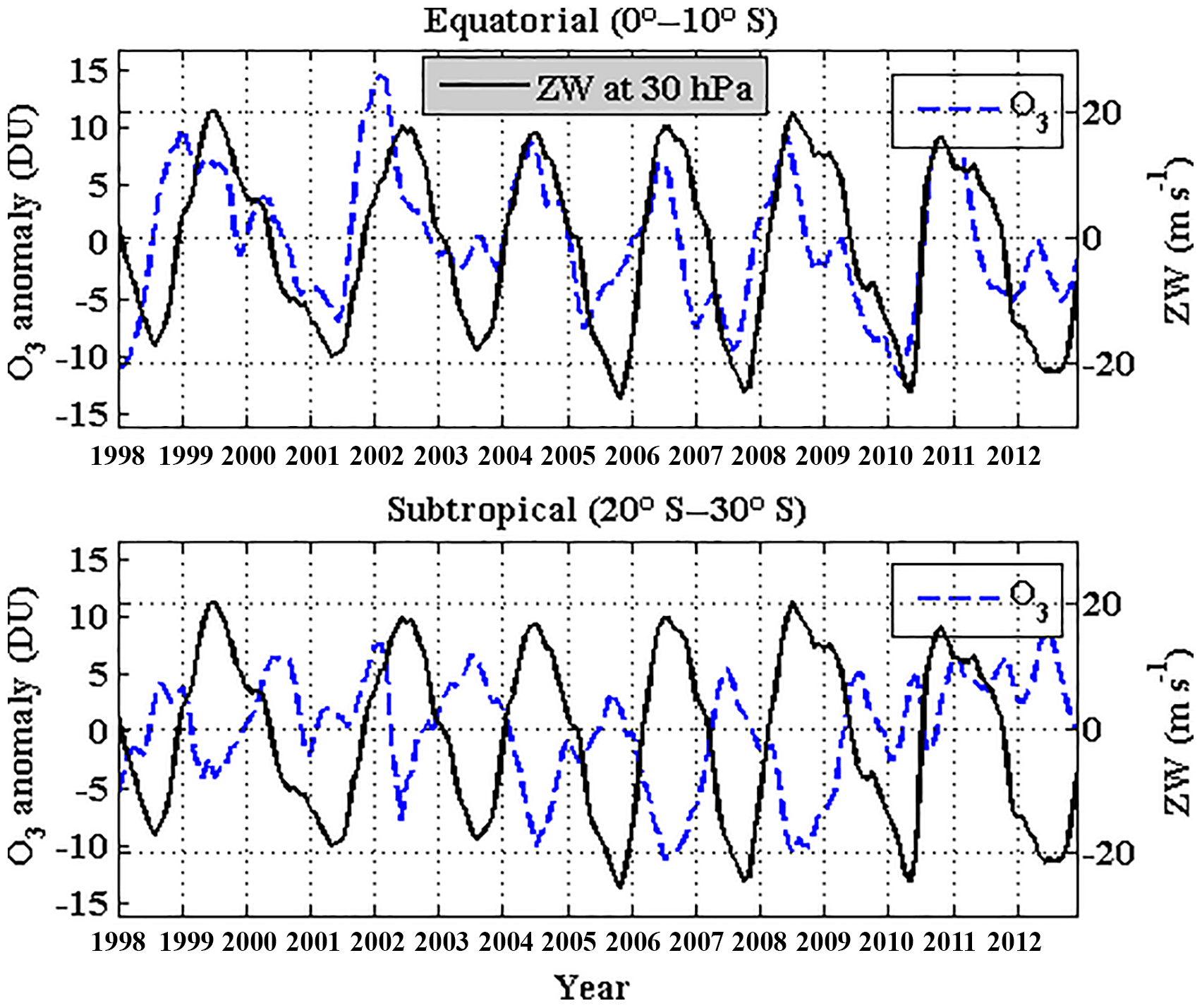
Figure 8Deseasonalized time series of total ozone (blue line) for equatorial (0–10∘ S) and subtropical (20–30∘ S) regions calculated by subtracting the ozone monthly mean from the corresponding monthly climatological value. The black line is the time series in months of zonal wind recorded at 30 hPa over Singapore.
The above process was explained by Peres et al. (2017) and may be outlined as follows: the descending westerly phases of the QBO are associated with a vertical circulation characterized by downward motion in the tropics and upward motion in the subtropics. This leads to a weakening of the normal speed of the Brewer–Dobson circulation. In this way the upward motion of air mass is slowed down and the tropopause height decreases. As the ozone mixing ratio increases with the increase in altitude in the lower stratosphere, ozone production can occur for a longer period than normal (Cordero et al., 2012). This mechanism leads to a positive column ozone anomaly at low latitudes and a negative anomaly in the subtropics. During the QBO descending easterly phase, ozone formed spends less time at low latitude due to the enhanced Brewer–Dobson circulation (Cordero et al., 2012). The newly created ozone is rapidly transported to the subtropics, resulting in a negative ozone anomaly at lower latitudes and a positive ozone anomaly in the extratropics.
Butchart et al. (2003) explained that the equatorial ozone anomalies due to QBO forcing extend to 15–20∘ of latitude. In order to investigate the border between equatorial and subtropical QBO signals on ozone, the response of the QBO signal to TCO variability for individual sites was calculated based on the regression coefficient associated with the QBO on the Trend-Run model (Eq. 4). The response values are given in column 5 of Table 5. It is seen that the response of QBO to TCO variability by unit of normalized QBO signal is positive when the QBO is in phase with the ozone signal and negative for the reverse case. In this study a positive response (of decreasing magnitude) is obtained with the decrease in latitude moving from Samoa (14.13∘ S) to Nairobi (1.27∘ S). Conversely the responses obtained are negative at Fiji (18.13∘ S), Reunion (21.06∘ S) and Irene (25.90∘ S). These results indicate that the border between the equatorial and subtropical QBO-ozone signature is found at around 15∘ in latitude. Similar results were reported by Chehade et al. (2014) by calculating the coefficients of regression associated with the influence of the QBO on ozone variability. The Chehade et al. (2014) study reported positive and negative regression coefficients between 0∘ and 15∘ S and from 15∘ S towards the pole respectively.
In this work, positive ozone anomalies with amplitude varying between 7.5 and 13.9 DU were recorded over the equatorial sites during the zonal wind westerly phase, while the negative anomalies observed during the easterly phase oscillated between −13.3 and −2.80 DU. These results indicate that inter-annual oscillations of TCO over the equatorial regions have maximum amplitude varying within ±14 DU during the study period (1998–2012). This is in agreement with the results of Butchart et al. (2003). For 1980 to 2000 they obtained a deseasonalized ozone signal which varied within ±14 DU over the Equator.
It is worth noting that the maximum amplitude of ozone anomalies observed in the subtropics is lower (within ±11 DU) than the equatorial region (±14 DU). These amplitude values indicate that the QBO modulation on inter-annual variability of ozone is higher over the equatorial region in comparison to the extratropics. Values reported in Table 4 show a clearly decreasing QBO contribution poleward, i.e. from Nairobi (20.48±1.92 %) in the equatorial zone to Irene (3.60±1.07 %) in the subtropics.
4.2.3 ENSO contribution
Column 6 of Table 4 presents the percentage of ENSO contributions to inter-annual ozone variability for individual sites. It is clear that the ENSO parameter does not exert much influence on ozone variability over the subtropical sites (Reunion and Irene), where its contribution to TCO variability is assessed to be less than 1 %. However, the ENSO contribution is more pronounced over tropical and low-latitude sites located between 19∘ S and the Equator. In this latitude band, the ENSO contributions observed at Fiji, Samoa, Ascension Island and Java are high compared to Natal and Nairobi. An average ENSO contribution of 9.40±0.65 % to total ozone variability over Fiji, Samoa, Ascension Island and Java is observed, while a corresponding value of 5.73±0.75 % for Natal and Nairobi is seen (see Table 4). These results indicate that the ENSO influence on total ozone variability is high over the tropics compared to that in the equatorial zone and subtropics. It has been reported by Randel et al. (2009) that ENSO originates in the tropics and is linked to coupled atmosphere–ocean dynamics. This factor may be the main reason for the observed high ENSO contribution over sites located in the tropics compared to low-latitude and subtropical sites. Zerefos et al. (1992) removed the QBO, seasonal and solar cycles from the ozone signal at Samoa and obtained a good correlation between ENSO and ozone signal. They mentioned a possible ENSO–ozone relationship beyond the tropical region only during very large ENSO events (e.g. 1982–1983, 1997). In this study, the low estimated ENSO contribution (less than 1 %) for the subtropical region may also be explained by the fact that there were few large ENSO events recorded during the investigated period (1998–2012).
The tropical sites located in the Pacific Ocean (Samoa, Fiji and Java) were more influenced by ENSO when compared to tropical and equatorial sites (Ascension Island, Natal and Nairobi) due to the high ENSO activity usually observed in the Pacific Ocean (Randel and Thompson, 2011; Chandra et al., 1998, 2007; Logan et al., 2008; Ziemke and Chandra, 2003; Ziemke et al., 2010). In addition, the Ascension Island ENSO contribution was higher compared to those observed at Natal and Nairobi. As ENSO is a coupling ocean–atmosphere event generated in the Pacific Ocean (Ziemke and Chandra, 2003; Rieder et al., 2013), the low ENSO contribution recorded over Natal and Nairobi compared to Ascension Island can be explained by their continental location. As Ascension Island is located in the Atlantic Ocean, the high ENSO contribution observed at this site is probably due to a Pacific–Atlantic Ocean connection.
The ENSO response to ozone variance is assessed and shown in the last column of Table 5. The aim of this work is to define the mean behaviour of ozone variance for individual sites during ENSO events. It is worth noting that the mean ENSO influence is observed on tropospheric ozone (Randel and Thompson, 2011; Ziemke and Chandra, 2003). However, due to weak variability in stratospheric ozone over the tropics (Ziemke et al., 1998) during periods of normal conditions, tropospheric ozone changes were shown to affect the stratospheric ozone and total column ozone variability over the tropics during ENSO events (Rieder et al., 2013). As the MEI is characterized by positive values during El Niño, a positive ENSO response indicates an increase in total column ozone (TCO) and a negative response indicates a decrease in TCO. The ENSO response to ozone variability over subtropical sites (Reunion and Irene) is positive, while it is generally negative over the tropics (except over Java and Nairobi). These results are in good agreement with those reported by Chehade et al. (2014) which are obtained using a regression analysis model. Through their study they obtained negative (positive) ENSO regression coefficients indicating a negative (positive) ENSO response to ozone variability over the tropics (extratropics). It has been mentioned in several papers (Rieder et al., 2013; Randel et al. 2009; Randel and Thompson, 2011; Frossard et al., 2013; Chehade et al., 2014) that a negative ENSO response to ozone variability in the tropics is linked to enhanced transport of an ozone-rich air mass from the tropics to the extratropics due to strengthening of the Brewer–Dobson circulation in the stratosphere during ENSO warm events. As reported by Rieder et al. (2013), ENSO events are associated with more frequent stratospheric warming, an increase in tropopause height and a decrease in stratospheric ozone in the tropics. By comparison, in the subtropics, the tropopause height decreases and stratospheric ozone increases. This effect could be the reason for the observed ENSO positive response over Irene and Reunion (subtropics). The ENSO warm events produce suppressed convective movements over the western Pacific, leading to a positive anomaly of ozone in this region, while the air mass convection is enhanced over the eastern Pacific that leads to a reduction of ozone (Ziemke and Chandra, 2003). For the period 1970–2001, Ziemke and Chandra (2003) obtained a positive El Niño response corresponding to an average peak of positive ozone anomaly evaluated at 5 DU over the Indonesia area. Furthermore, they found a negative ozone anomaly in the eastern Pacific, the location of Fiji and Samoa. According to Ziemke and Chandra, (2003), this could be the main reason for the observed positive ENSO response at Java in the western Pacific and negative response over Samoa and Fiji in the eastern Pacific. The connection between the western Pacific and the Indian Ocean could be among the reasons for the observed positive ENSO response to ozone variability at Nairobi in the eastern African and Reunion in the western Indian Ocean region.
4.2.4 Solar flux contribution
Variation in total ozone concentration also depends on solar flux intensity over the tropics and subtropics. Figure 9 illustrates the variation in annual total ozone anomaly calculated between 1998 and 2012 over the three regions (bottom panel) and the annual 10.7 cm solar radio flux variation during the same period (top panel). Inspection of Fig. 9 illustrates the effect of the 11-year solar cycle on inter-annual total ozone variations. Negative ozone anomalies are observed during periods of low sunspot intensity, thereby confirming the dependence of ozone production on incident solar radiation flux. The converse is also true; that is, high annual total ozone levels are associated with periods of high sunspot intensity. The results presented here are in good agreement with Soukharev and Hood (2006). The latter obtained negative (positive) monthly mean ozone anomalies during periods with low (high) Mg II solar UV intensity. The dependence of annual ozone levels on annual solar radiation is also highlighted by Efstathiou and Varotsos (2013). In this investigation, the high levels of TCO were observed over the tropics when solar activity was at a maximum (2001) and compared to values recorded during a minimum in solar activity in 2008. This illustrated the impact of the solar cycle on global ozone concentrations. In the work presented here, considering the year with solar maximum (2001) to the year with minimum solar intensity, a variation in ozone levels was observed corresponding to approximately 1.05, 1.52, and 1.60 % for the (a) equatorial, (b) tropical and (c) extratropical regions respectively. It is expected that the observed percentage change in ozone levels is directly related to solar flux activity. A study by Zerefos et al. (1997) confirmed that the solar flux component in TCO between 1964 and 1994 was approximately 1–2 % over decadal timescales. It can therefore be concluded from the results presented here, together with those of Zerefos et al. (1997), that the solar flux contribution to ozone variability did not vary significantly during the past 6 decades.
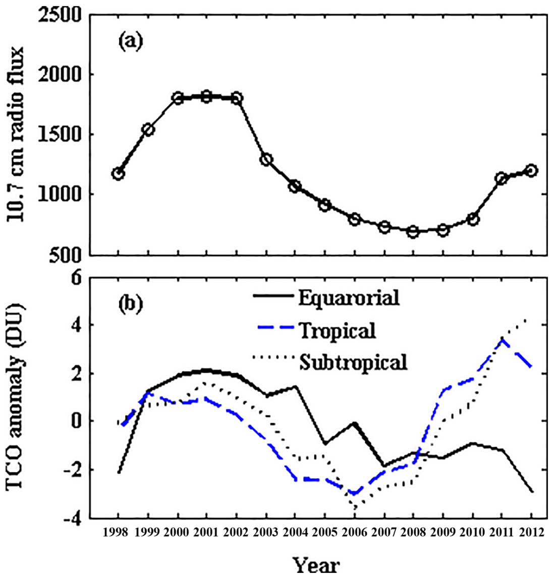
Figure 9(a) Annual mean of 11-year solar flux recorded from 1998 to 2012 and (b) the annual TCO anomaly recorded for the same period in equatorial, tropical and subtropical regions.
As the solar flux index is one of the input parameters in the regression model, the contribution and response of the 11-year solar cycle to total ozone variability were assessed. The effect of changes in solar flux on ozone levels is presented in the fourth column of Table 5. The obtained responses are always positive, indicating that the solar flux index is in phase with total ozone time evolution as reported in the WMO (2014). The increase in ozone occurs when the sunspot intensity increases and vice versa. The average magnitude of the solar flux response to ozone variability is about 1.57 % by unit of solar flux index. The contribution of solar flux to total ozone variability over the study region varies by between approximately 4.38 and 7.81 %. The contribution of the solar cycle is high compared to the 3 % reported by the WMO (2010, 2014) on the global scale. This is probably due to (1) the length of the data records (less than two solar cycles), (2) the time period under investigation (1998–2012) and (3) the studied region (from equatorial to around 40∘ S). However, the contribution values obtained exhibit a minimum at Reunion in the subtropics and a maximum at Ascension Island in the lower-latitude region. These results indicate a high solar flux influence over the low-latitude region in comparison with the subtropics. The contribution of solar flux to total ozone variability decreases gradually by moving away from Ascension Island equatorward or southward. This solar flux contribution pattern is similar to that observed in semi-annual oscillations (see Sect. 4.2.1). From the results presented in this study it can be inferred that semi-annual variations are modulated by solar activity over the tropics and subtropics and that both semi-annual and 11-year solar forcings control ozone distributions.
4.3 Height profile ozone variability
The main objective of this section is to provide additional details regarding the contribution of proxies to ozone variability for different altitude levels from 15 to 30 km. This exercise is based on vertical distribution of ozone concentration as presented in Fig. 4. Here the ozone profiles are interpolated with 0.1 km vertical resolution giving 150 altitude levels in the 15–30 km altitude range. The Trend-Run model is applied to each altitude level.
4.3.1 Seasonal contribution to ozone profile variability
The contributions of annual and semi-annual oscillations to ozone variability (15 to 30 km) are shown in Fig. 10. Figure 10 reveals that seasonal cycles are the most dominant forcings to ozone variability in the lower stratosphere. The contribution of annual oscillation (AO) to ozone variability is highlighted over the three studied regions and accounts for more than 40 % in the UT–LS (upper troposphere–lower stratosphere). AO maximum amplitudes in equatorial and tropical regions are found around the tropical tropopause layer (TTL) below 20 km and around 22.5 km in the subtropics. These results are in good agreement with recent findings. Gebhardt et al. (2014) showed that in the lower stratosphere (21 km), ozone variability is dominated by AO in the tropics (20∘ N–20∘ S). Furthermore, Eckert et al. (2014) explained that vertical motion in the TTL had a significant impact on ozone variance and that seasonal variations contributed more than 50 % to ozone variability in this layer. A strong annual cycle signature in the UT–LS has also been reported by Bègue et al. (2010). The important contribution of the annual cycle in the UT–LS may be due to the STE (stratosphere–troposphere exchange) processes which occur seasonally in the tropics. These exchanges are linked to the upwelling air mass through the tropopause in summer and the submersion of stratospheric air mass to the troposphere during winter. These air mass exchanges affect the seasonal budget of ozone and temperature from equatorial to middle latitude. As seen in Fig. 10, annual cycle contributions higher than 40 % are found from 15 to 20 km over the equatorial region. However, the annual cycle contributions higher than 40 % observed over the tropical region are found from 17.5 to 22 km. In addition, the maximum annual cycle contribution for the equatorial region is observed at 18.5 km, whilst in the tropics it occurs at 19.5 km. These observations support the existence of upward propagation of the AOs of ozone below 25 km and the amplitude of these AOs increases with the increase in latitude poleward. This may explain the high annual cycle contribution observed in the 15–24.7 km altitude range in the subtropics. The presence of an annual signature in ozone temporal evolution in this wide altitude band (15–24.7 km) in the subtropics is inconsistent with the strong annual variability observed in TCO, as discussed in the previous subsection.
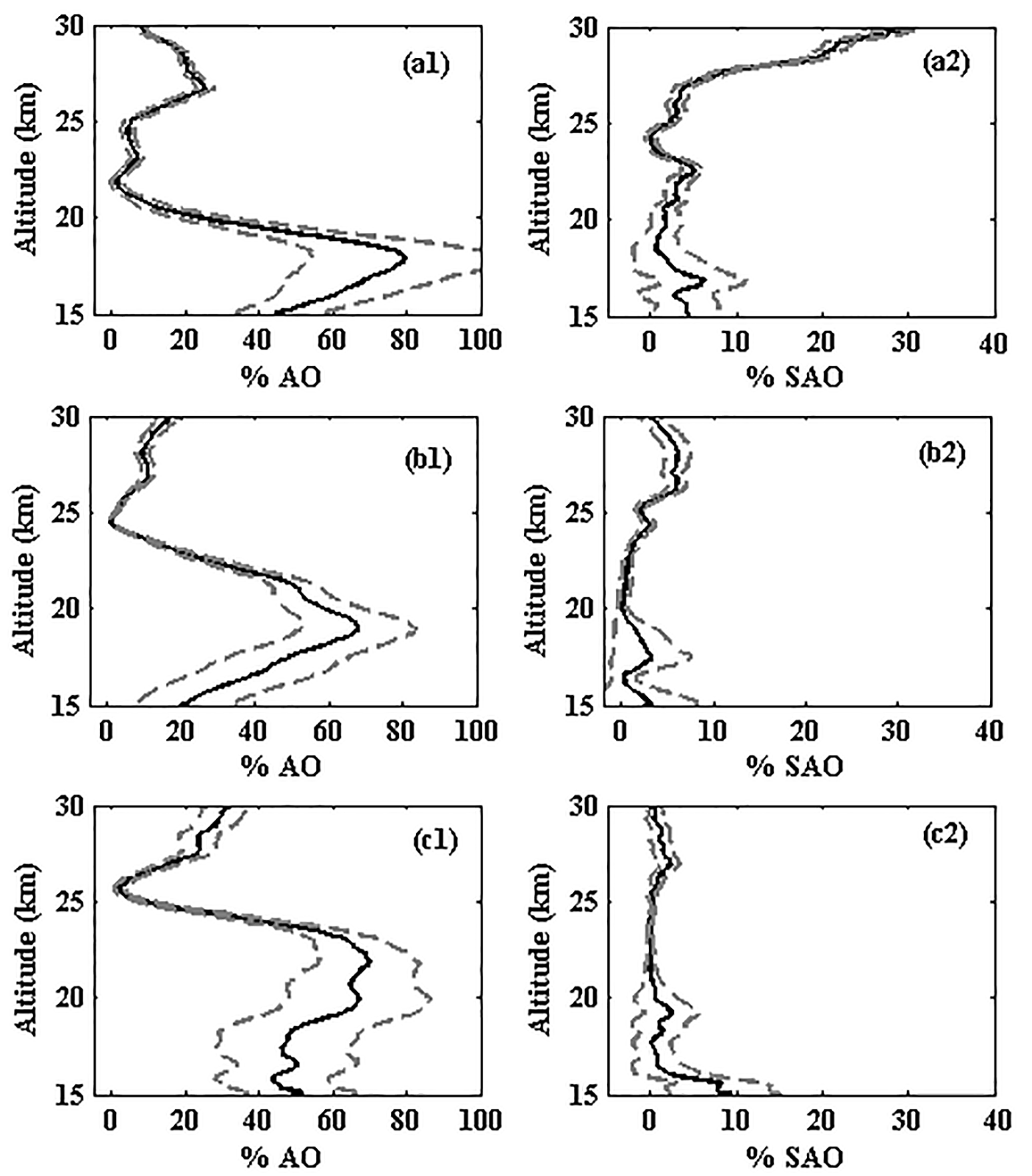
Figure 10Height profile in % of the contribution of the annual cycle (a1–c1) and the semi-annual cycle (a2–c2) to ozone variability as calculated by the Trend-Run model over the equatorial (a1, a2), tropical (b1, b2) and subtropical (c1, c2) regions. SDs associated with contributions are presented in grey dotted lines.
It is worth noting that the seasonal cycles of ozone observed at altitudes below 25 km are linked to dynamical processes, while above an altitude of 27 km, seasonal cycles are modulated by ozone photochemical processes. Contributions of the annual forcing of greater than 10 % are observed at altitudes above 27 km. Here the contribution part of annual oscillation increases with altitude, especially over the tropical and subtropical regions. These results support the existence of an annual cycle signature on ozone temporal evolution over altitudes above 30 km in the tropical and subtropical regions. Eckert et al. (2014) found that ozone variation due to AO was greater than 10 % above 27 km in the 10–30∘ S latitude band. However, this amplitude decreases above 35 km, where ozone variability is strongly controlled by semi-annual oscillation (SAO). Furthermore, the maximum amplitude of the ozone SAO signal observed by Eckert et al. (2014) was centered slightly above 30 km over the tropics. Mze et al. (2010) observed a strong semi-annual cycle in equatorial ozone climatology between 27 and 36 km, with a maximum peak at 31 km, and Gebhardt et al. (2014) observed ozone variability dominated by SAO in the middle (35 km) and upper tropical stratosphere (44 km) in the tropics (20∘ N–20∘ S).
The (SAO) contribution to ozone variability is highlighted in the present work for altitudes higher than 27 km for the equatorial and tropical regions. Above 27 km, the SAO contribution accounts for more than 10 % of total ozone variability over the equatorial region, while this effect is reduced to less than 10 % for the tropics. This confirms the high contribution of SAO to ozone variability at low latitudes with respect to other regions as discussed in Sect. 4.1.1. As supported by Eckert et al. (2014), beyond the tropics the SAO amplitude decreases gradually to near zero. As reported in previous studies, the SAO is linked to change in the zonal wind regime at the equatorial stratopause, where the maximum component appears during solstice (when easterly) and equinox (when westerly) (Belmont, 1975; Hirota, 1978; Delisi and Dunkerton, 1988). This mechanism leads to temperature anomalies corresponding to 2–4 K in the upper stratosphere (Nastrom and Belmont, 1975), thereby driving a change in the rate of ozone production and loss (Maeda, 1984) during the solstice and equinox periods. As demonstrated in Sect. 4.2.1, the equinox period is characterized by maximum peaks of TCO production over the equatorial region, while the solstice corresponds to minimum ozone levels (or ozone loss) over equatorial regions.
4.3.2 QBO contribution to ozone profile variability
QBO contributions to ozone profile variability between 15 and 30 km are presented in Fig. 11 for the three regions, namely (a1) equatorial, (b1) tropical and (c1) subtropical. A strong contribution of the QBO to ozone variability is observed over the 20–28 km altitude range for the equatorial region. Here the QBO is the most dominant mode and accounts for more than 30 % of ozone variability. These results are in agreement with previous work in which a strong signature of the QBO on inter-annual variability of ozone with large amplitudes over the tropics at altitudes of approximately 20–27 km has been reported (Randel and Thompson, 2011; Gebhardt et al., 2014; Eckert et al., 2014). Figure 11a1 shows two strong peaks at 60 % corresponding to altitudes of 21.5 and 25 km. The QBO contribution is important and does not change much over the altitude range 24 to 26.5 km, indicating that the maximum amplitude of the QBO signature occurs in this altitude range, where the degree of QBO influence on ozone variability is approximately invariant. Fadnavis and Beig (2009) found the QBO maximum over tropics at approximately 26 km, while Eckert et al. (2014) found this maximum at 25 km. The QBO signal on ozone variability is linked to the downward propagation of zonal wind throughout the time. This process leads to a positive (negative) ozone anomaly when in the westerly (easterly) mode with a cycle of around 2 years (Randel and Thompson, 2011; Lee et al., 2010; Butchart et al., 2003). Note that the maximum contributions of the QBO over the tropical and subtropical regions (Fig. 11b1 and c1) are less than 12 %. These results confirm the latitudinal signature of the QBO which is expressed by a decrease in its effect on ozone variability poleward. The inter-annual ozone anomaly linked to the QBO time evolution can be positive or negative depending on the altitude range for a given period due to the downward propagation pattern of the QBO with time (Randel and Thompson, 2011). The responses of the QBO index used are presented in Fig. 11 as (a2) equatorial, (b2) tropical and (c2) subtropical regions. Over the equatorial region, the QBO index profile exhibits positive values below 23 km and negative values above. These results indicate a strong contribution of the QBO westerly regime to ozone variability for equatorial regions below 23 km during the studied period (1998–2012). In contrast, the easterly regime had more influence on variability of ozone above altitudes of 23 km. The opposite case is observed in the subtropics, where the QBO index profile exhibits positive values for altitudes between 18 and 23 km and negative values between altitudes of 23 to 27.5 km. Similar results have been reported by Bourassa et al. (2014). The response amplitude obtained in this work over the subtropics varies within ±5 %, whilst it is at ±7 % (by unit of the normalized QBO index) over the equatorial region. These results reaffirm the key role of the QBO in ozone variability highlighted in equatorial regions in contrast to the subtropics.
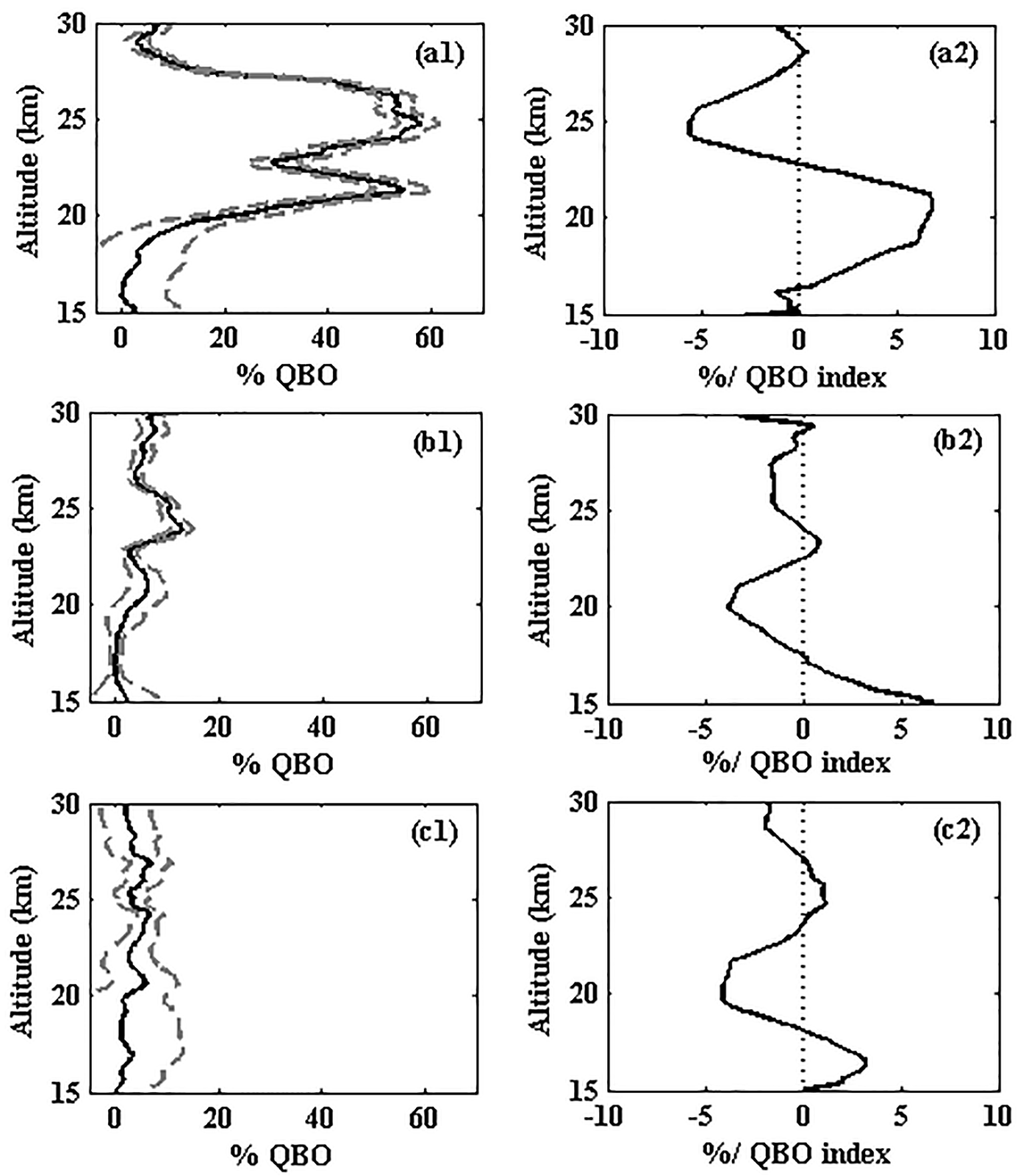
Figure 11Height profile in % of the QBO contribution of (a1–c1) and response by unit of the QBO index (a2–c2) as calculated by the Trend-Run model over the equatorial (a1, a2), tropical (b1, b2) and subtropical (c1, c2) regions. SDs associated with contributions are presented in grey dotted lines.
4.3.3 ENSO contribution to ozone profile variability
ENSO contributions to ozone profile variability over the 15–30 km altitude range are presented in Fig. 12 for the three regions (a1) equatorial, (b1) tropical and (c1) subtropical. These calculations show that ENSO events weakly affect subtropical ozone levels. In contrast, the ENSO contribution and its associated response to ozone variability appear to be important below an altitude of 25 km at tropical latitudes. These results are in good agreement with the study by Sioris et al. (2014) in which a statistically significant ENSO contribution was reported at an altitude of 18.5–24.5 km in the tropics. Such results indicate that ENSO influence on ozone variability is essentially focused on the troposphere and lower stratosphere. ENSO contribution to the lower stratospheric ozone is highlighted by the 20–25 km altitude band with peaks toward 15 and 13 % over the tropical (at 23 km) and equatorial (at 21 km) regions respectively. The response linked to this contribution over the equatorial region oscillates with amplitude, varying between −8 and 4 % (Fig. 12, curve a2). Here the ENSO response values are negative below an altitude of 23 km and positive in the 23–26 km altitude range, indicating that the multivariate ENSO index is in phase with ozone time evolution above 23 km and in opposite phase below 23 km. As reported in previous studies (Ziemke and Chandra, 2003; Rieder et al., 2013), ENSO events contribute to the variation in tropopause height associated with decrease/increase in TCO due to the enhancing/suppressing of tropical convection. The results obtained in the equatorial region indicate that the ENSO effect, associated with enhanced convection, generally affects the lower part of the stratosphere. This leads to a decrease in ozone levels below 23 km, while the suppressed convection present generally results in a positive response to ozone variance above 23 km.
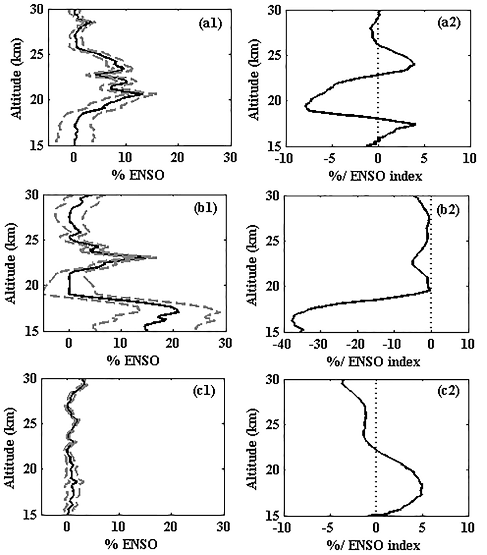
Figure 12Height profile in % of the contribution of ENSO (a1–c1) and response by unit of the ENSO index (a2–c2) as calculated by the Trend-Run model over the equatorial (a1, a2), tropical (b1, b2) and subtropical (c1, c2) regions. SDs associated with contributions are presented in grey dotted lines.
However, the amplitude obtained for the negative ENSO response is the largest. These results suggest that ozone variability linked to ENSO events is more sensitive to the enhanced equatorial convection in the UT–LS. In a recent study, similar results were reported by Randel and Thompson (2011), in which they observed a large negative change in ozone variance due to enhanced Brewer–Dobson circulation over the tropics associated with ENSO variability. In addition, the obtained ENSO response over the tropical region (Fig. 12b2) is negative, indicating a decrease in ozone due to ENSO events occurring during the study period. From the troposphere to approximately 20 km, the ENSO signal exhibits an important contribution and response to ozone variability over the tropics as reported in previous published works (Bourassa et al., 2014; Sioris et al., 2014; Randel and Thompson, 2011). However, the response obtained has a larger amplitude (maximum of −38 % at 16.5 km) than those reported by the above-mentioned papers due to the location of the Fiji and Samoa stations (the two sites that represent the tropical region in this work). As mentioned above, Fiji and Samoa are located in the eastern Pacific, a region where ENSO events are significant. Here the ENSO contribution to total ozone variability is observed to be greater than 10 % below 18.7 km. The negative ENSO response associated with this contribution is explained by an enhanced tropical upwelling during ENSO events which led to a decrease in ozone levels in the lower stratosphere of the eastern Pacific Ocean region as reported by previous studies (Randel and Thompson, 2011; Randel et al., 2009; Calvo et al., 2010).
4.4 The trend estimates
4.4.1 Total column ozone trends
The trend analysis of TCO was performed for each site and results presented in Fig. 13. The TCO trends are assessed based on the Trend-Run model and expressed in percentage per decade. The obtained trend values are positive, suggesting an increase in TCO during the study period. However, the mean values of TCO trends obtained from the Samoa site (14.13∘ S) equatorward are lower than 1 %, while they are higher than 1.5 % for Fiji (18.13∘ S), Reunion (21.06∘ S) and Irene (25.90∘ S). These results illustrate that the increase in TCO in the subtropics is greater than in the tropics. Figure 14 summarizes the trend evolution over the three latitudinal bands. An increase in the trend with latitude southward is observed. The average trends (in percentage per decade) are , and (±1σ) over the equatorial, tropical and subtropical regions respectively. These TCO trend results are consistent with the WMO (2014), where a positive trend of approximately 1±1.7 (±2σ) was reported at 60∘ N–60∘ S for the period 2000–2013. These positive trends are probably linked to the decline of effective equivalent stratospheric chlorine (EESC) over the globe as supported by previous studies (Yang et al., 2006; Anderson et al., 2000; Waugh et al., 2001; WMO 2010). However, compared with the tropics and subtropics, the delay in ozone improvement observed in the equatorial region is probably due to the tropical strengthening of the Brewer–Dobson circulation (WMO 2014; Randel and Thompson, 2011).
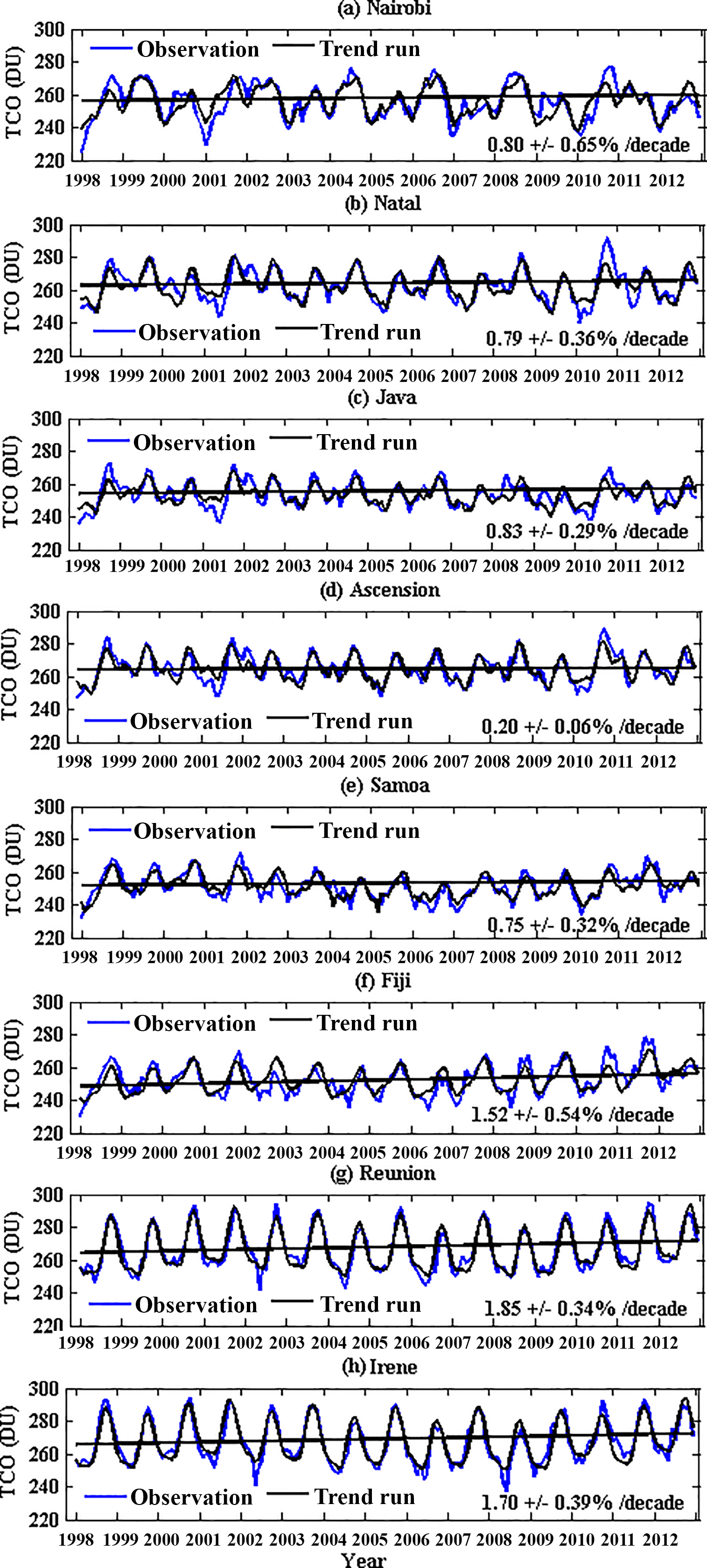
Figure 13Time evolution of monthly total ozone values (blue) observed at each site. The black lines represent the time evolution of the TCO obtained by the Trend-Run model, the blue lines show observation data, and the straight black line illustrates the obtained decadal trend.
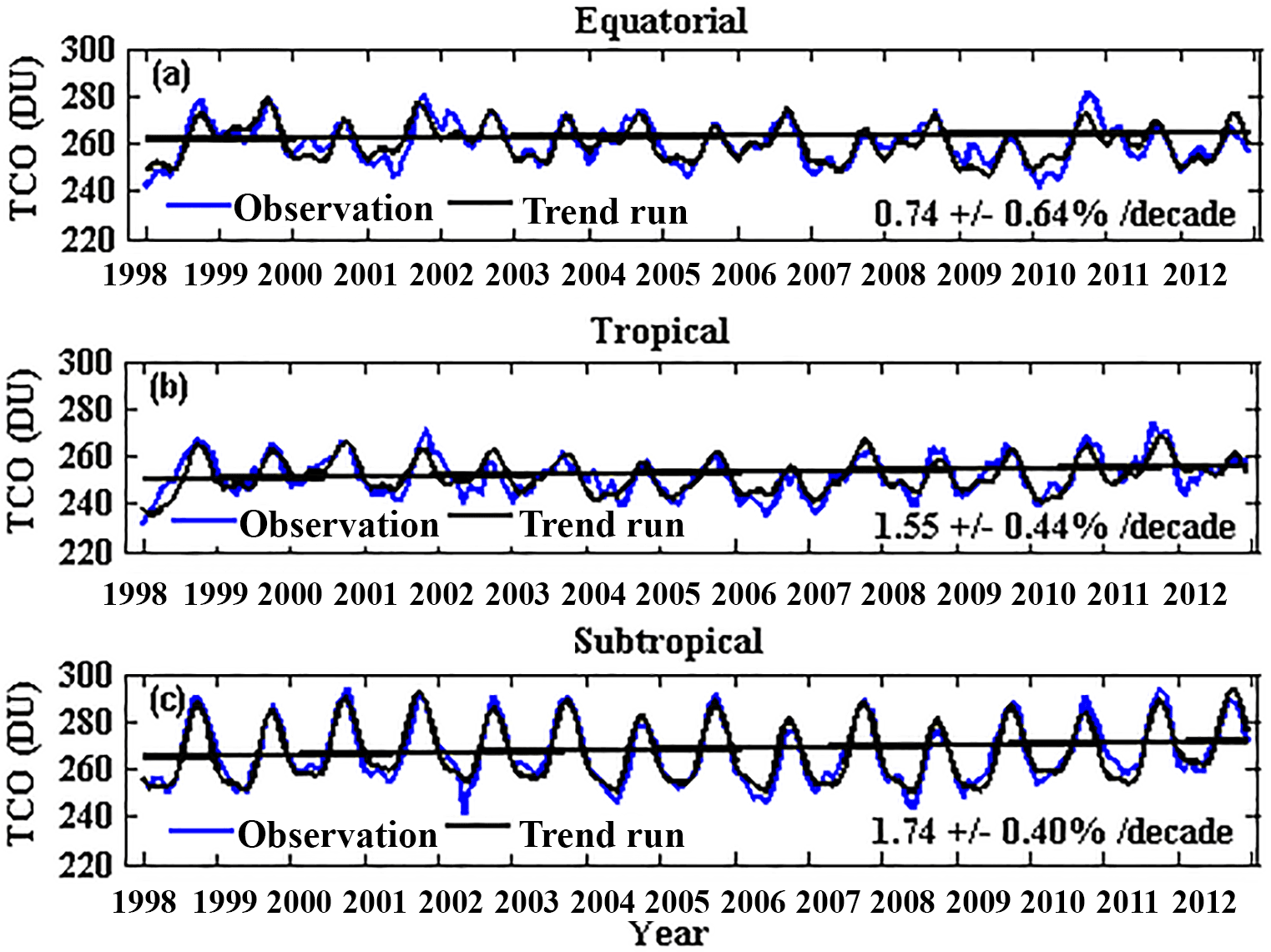
Figure 14The same as Fig. 13 but per latitudinal region: equatorial (a), tropical (b) and subtropical (c).
It should be noted that approximately 10 % of ozone is tropospheric and is produced as a result of chemical reactions between species such as nitrogen oxide (NOx), carbon monoxide (CO) or volatile organic compounds (VOCs). In the context of climate change due to anthropogenic pollutant emissions and in spite of the efforts by the international community to reduce GHG emissions, pollution has continued to increase in the Southern Hemisphere, leading to a systematic increase in tropospheric ozone. Thompson et al. (2014) assumed that growth in ozone precursors like NOx and VOC may account for the characteristic free tropospheric ozone increase, especially in wintertime. The observed positive trend in TCO time series is therefore probably due also to an increase in and long-range transport of pollutants (mainly from industrial and biomass burning activity) in the free troposphere of the southern tropics and subtropics, as suggested by previous studies (Diab et al., 2004; Thompson et al., 2014; Clain et al., 2009). Thompson et al. (2014) highlighted significant increases throughout the free troposphere, 20–30 % decade−1 over Irene and up to 50 % decade−1 over Reunion in the southern subtropical region.
Furthermore, Heue et al. (2016) showed that the tropical tropospheric ozone trend is 0.7±0.12 DU (approximately 3.5 %) decade−1 between 1995 and 2015. There results show that there is an improvement in ozone from the ground to the middle atmosphere in the studied regions. Tropospheric ozone affects total column ozone trends; however, the contribution is not sufficient to modify the TCO trend compared to stratospheric ozone, which represents 90 % of the total ozone present.
4.4.2 Vertical distribution of the trends
In this investigation, TCO analysis indicated a positive trend over the study region. However, a trend investigation in terms of vertical ozone distribution is necessary in order to understand trend variation through different altitude levels. Equatorial, tropical and subtropical ozone trend profiles estimated by the Trend-Run model are presented in Fig. 15, panels (a), (b) and (c) respectively. Considering the temporal coverage of Irene ozonesonde data (1998–2008 and some profiles recorded in 2012), the Irene and Reunion ozone profiles were separated for the sake of trend analysis. Figure 15c1 shows the ozone trend profile for Reunion, while that for Irene (January 1998 to December 2008) is shown in panel c2. Overall, the ozone trends obtained are negative in the upper troposphere and positive for altitudes higher than 22 km. This indicates an improvement in stratospheric ozone. For the equatorial region, the trend profile shows a positive gradient from 15 km to the tropopause (approximately 18 km), followed by a maximum positive ozone trend in the 18–22 km layer (about +2 %). A negative trend is seen between 22 and 25 km and a zero trend for heights above 25 km. The tropical trend evolution below 22 km is similar to the trend observed over Reunion (Fig. 15c1), which is marked by a negative peak around 19 km. Such a negative peak is probably a characteristic of the tropical trend and highlighted at Reunion due to the proximity of this station to the tropical zone.
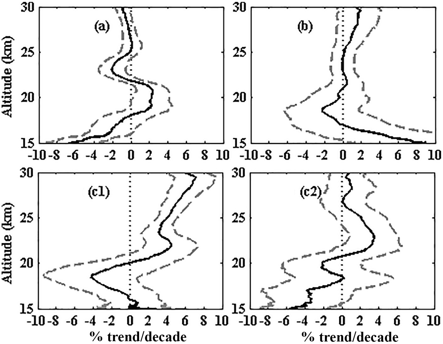
Figure 15Vertical profiles of ozone decadal trends derived by the Trend-Run model from 15 to 30 km at the Equator (a), tropics (b), Reunion (c1) and Irene (c2). Irene and Reunion are separated for this present case due to the lack of ozone profiles at the Irene station from January 2008 to October 2012. The Irene trend profile is derived based on ozone profiles recorded from January 1998 to December 2007 (10 years).
The results in trend estimates over the equatorial region are similar to previous studies based on a combination of GOMOS and SAGE II data recorded between 1984 and 2011 performed by Kyrölä et al. (2013). This work showed an apparent improvement in ozone trends onwards from 1997. The recorded trend (1997–2011) in the 20–30 km altitude range is consistent with results obtained in the present study and can be summarized as follows: a positive trend of approximately 2 % in the altitude range 19–21 km and approximately 0 % between altitudes 21 and 30 km. A trend varying between 0 and 1 % was also observed by Randel and Thompson (2011) in an altitude range of 23 to 35 km by averaging SHADOZ and SAGE II ozone profiles recorded between 1984 and 2009 for latitudes 20∘ N–20∘ S. Furthermore, Randel and Thompson (2011) observed a negative peak at 19 km, similar to what was observed in this study over Reunion and the tropical region. This negative peak is explained as resulting from a systematic increased tropical lower stratospheric upwelling. As reported by the WMO (2014), the increase in tropical upwelling is associated with a strengthening of the Brewer–Dobson circulation caused by GHG-induced climate change. Furthermore, Lamarque and Solomon (2010) associated the declining trend in ozone levels in the lower tropical stratosphere with an increase in carbon dioxide and sea surface temperature. They also demonstrated that a decrease in ozone in the upper stratosphere could be strongly linked to an increase in halogen compounds at high altitudes. The results obtained in this work indicate that the positive trends observed over Reunion and Irene from TCO analyses are probably due to an increase in ozone levels in the stratosphere, which is associated with a decrease in halogen compounds and EESC at high altitudes. Declining EESC levels in the subtropical region constitutes the main reason for ozone increase as a result of the Montreal Protocol and its amendments (Yang et al., 2006; Anderson et al., 2000; Reinsel, 2002; WMO, 2010, 2014).
The positive trend of 2 % in ozone levels recorded over the equatorial region in the 18–22 km altitude range cannot be explained by the decline of EESC compounds in the stratosphere. Instead, this trend could rather be linked to an increase in NOx (NO+NO2) in this altitude range (Gebhardt et al., 2014; Nevison et al., 1999). Furthermore, Gebhardt et al. (2014) obtained a positive ozone trend at altitudes higher than 18 km and the variation pattern observed is similar to that obtained in our study up to an altitude of approximately 23 km. The investigation of Gebhardt et al. (2014) was based on SCIAMACHY satellite observations (2002–2012). They associated the observed positive trend at 18–22 km with an increase in NOx concentration in the lower stratosphere. The idea that NOx levels may have a direct effect on stratospheric ozone variability is not new and was first suggested by Nevison et al. (1999). In this study they used a model in order to identify the NOx contribution to ozone variability at different altitudes in the stratosphere. Through these calculations it was found that the increase in NOx compounds in the lower stratosphere leads to an increase in ozone levels at this altitude. It is important to note that NOx can have a buffering effect on the Clx and HOx ozone-destruction cycles in the tropical lower stratosphere as explained by Nevison et al. (1999).
This work describes and discusses the variability and associated trends in ozone measurements recorded between January 1998 and December 2012 over eight southern tropical and subtropical sites. Total ozone products from different instruments were presented and a very good agreement was found in products recorded by different instruments at the same site. This confirmed the good quality of products and the validity of combining these products in order to create a long-term and homogenous TCO dataset for the study of ozone variability and long-term trends over the southern tropics and subtropics. SHADOZ data, used for the study of vertical ozone distribution, were found to be good quality according to Thompson et al. (2003a, b). The analysis of the contribution and response of some parameters to total ozone variance was achieved through the use of a multi-regression model called Trend-Run. This model is able to describe 71–91 % of ozone variability influenced by seasonal variation of climate and by dynamic parameters such as QBO, ENSO and solar flux. The obtained results were found to be in good agreement with recent findings and can be summarized as follows.
-
Ozone variability over the study region is dominated by annual oscillation (AO) which strongly affects ozone variance in the UT–LS as a result of seasonal troposphere–stratosphere exchanges. The amplitude of ozone annual oscillations is high in the subtropics and decreases with latitude equatorward. In contrast, the ozone SAO is more apparent and contributes significantly above 27 km, with its maximum influence at the lower latitudes (around 8∘ S), where its amplitude decreases with movement toward the Equator or subtropics.
-
The QBO signal constitutes the second most important parameter in terms of effect on ozone variability in the tropics after the seasonal oscillation. QBO heavily affects ozone variance in 20–28 km of the altitude range, with its maximum amplitude in the equatorial region. The pattern of the QBO response to ozone variability in the equatorial region is out of phase with that of the subtropics. The border between equatorial and subtropical patterns is found at around 15∘ in latitude.
-
The ENSO contribution over the subtropics is less than 1 %. In contrast, an important contribution of ENSO to ozone variance is highlighted in the tropics, below 25 km with its maximum amplitude in the Pacific area. The tropical ENSO response is basically negative and was explained in previous work (Randel and Thompson, 2011; Sioris et al., 2014) as resulting from an enhancement of tropical convection leading to ozone decrease during warm ENSO events.
-
Solar flux and total ozone are in phase. Increase in ozone levels occurs when sunspot intensity increases and conversely periods of low sunspot activity correspond to periods of low ozone production. The maximum solar flux contribution is at the tropical latitudes. The mean contribution of solar flux to total ozone variability over the studied region is high (6.03±0.84 %) compared to the 3 % reported globally by the WMO (2010, 2014). This is probably due to the region selected for this study (tropics and subtropics), the length of the data records (less than two solar cycles) and the time period under investigation in this work (1998–2012).
The regression model is also used to quantify ozone trends over the selected regions. Results obtained exhibit an upward trend of TCO during the period of study. The trend values were in good agreement with the WMO (2014) report (1±1.7 (2σ) at 60∘ N–60∘ S for the period 2000–2013) and exhibited an increase in ozone with increase in latitude from the Equator to the subtropics. The results of vertical profile analysis illustrated a positive ozone trend from 22 km upward and negative values in the upper troposphere, indicating that the ozone recovery observed in tropical and subtropical regions occurs in the stratosphere. It has been explained in recent studies (Sioris et al., 2014; Bourassa et al., 2014; Randel and Thompson et al., 2011) that the delay in ozone recovery at upper tropospheric and lower stratospheric levels was partly associated with a tropical enhancement of the Brewer–Dobson circulation over the tropics, while ozone recovery observed from an altitude of 22 km and upward was probably linked to declining levels of stratospheric chlorine and bromine compounds in the atmosphere. A further study continuing from this work would involve the inclusion of Brewer–Dobson and EESC indexes in the model not only to quantify the sources of observed trends, but also to improve the model quality.
AMT was the project leader; TP was the supervisor of the project; VS and HB participated in interpretation of the results and the review of the manuscript; AP and NB contributed to data analysis and the review of the manuscript.
The authors declare that they have no conflict of interest.
The data used in the present work are available and publicly accessible from different sites: Dobson and SAOZ TCO data, available at https://woudc.org/data/explore.php; TOMS TCO data, available at https://acdisc.gesdisc.eosdis.nasa.gov/opendap/ EarthProbe_TOMS_Level3/TOMSEPL3.008/contents.html; OMI data, available at https://gs614-avdc1-pz.gsfc.nasa.gov/pub/data/satellite/Aura/OMI/V03/L2OVP/OMTO3/; SHADOZ ozonesonde data, available at https://tropo.gsfc.nasa.gov/shadoz/Archive.html; ENSO, solar, and QBO flux indexes, available at https://www.esrl.noaa.gov/psd/data/climateindices/list/.
This article is part of the special issue “Space weather connections to near-Earth space and the atmosphere”. It is not associated with a conference.
The LACy (Laboratoire de l'Atmosphère et des Cyclones) is
supported by the INSU (Institut National des Sciences de l'Univers),
a CNRS institute, and by the Regional Council of Reunion (Conseil
Regional de La Réunion). This present work is supported by the
RAMI project, a regional doctoral school in the Indian Ocean zone,
under the “Horizons Francophones” programme of the AUF (Agence
Universitaire de la Francophonie) and the GDRI-ARSAIO (Atmospheric
Research in Southern Africa and the Indian Ocean), a French–South
African cooperative programme network supported by the French Centre National
de la Recherche Scientifique (CNRS) and the South African
National Research Foundation (NRF). The first author
(Abdoulwahab Mohamed Toihir) acknowledges the Indian Ocean Bureau of
AUF and the University of KwaZulu Natal for travel and hosting under
invited student exchange in the above NRF-CNRS bilateral research
project (UID 68668). The authors also thank Barbara Lynn Duigan
(NASSP-UKZN) for improving the readability of the manuscript. The
authors are thankful to agencies supporting NDACC activities:
INSU/CNRS, CNES as well as the Canada WOUDC team, which is under the
auspices of the WMO, the SHADOZ network, and the OMI and TOMS programmes, for
providing access to data via their websites.
Edited by: Petr Pisoft
Reviewed by:
Lucas Vaz Peres and two anonymous referees
Anderson, J., Russell III, J. M., Solomon, S., and Deaver, L. E.: Halogen occultation experiment confirmation of stratospheric chlorine decreases in accordance with the Montreal Protocol, J. Geophys. Res., 105, 4483–4490, 2000.
Antón, M., Loyola, D., Clerbaux, C., López, M., Vilaplana, J. M., Bañón, M., Hadji-Lazaro, J., Valks, P., Hao, N., Zimmer, W., Coheur, P. F., Hurtmans, D., and Alados-Arboledas, L.: Validation of the MetOp – a total ozone data from GOME-2 and IASI using reference ground-based measurements at the Iberian Peninsula, Remote Sens. Environ., 115, 1380–1386, 2011.
Austin, J., Tourpali, K., Rozanov, E., Akiyoshi, H., Bekki, S., Bodeker, G., Brühl, C., Butchart, N., Chipperfield, M, Deushi, M., Fomichev, V. I., Giorgetta, M. A., Gray, L., Kodera, K., Lott, F., Manzini, E., Marsh, D., Matthes, K., Nagashima, T., Shibata, K., Stolarski, R. S., Struthers, H., and Tian, W.: Coupled chemistry climate model simulations of the solar cycle in ozone and temperature, J. Geophys. Res., 113, D11306, https://doi.org/10.1029/2007JD009391, 2008.
Basher, R. E.: Review of the Dobson Spectrometer and its Accuracy in Atmospheric Ozone, edited by: Zerefos, C.S and Ghazi, A., Reidel and Dordrect, 387–388, 1985.
Bègue, N., Bencherif, H., Sivakumar, V., Kirgis, G., Mze, N., and Leclair de Bellevue, J.: Temperature variability and trends in the UT-LS over a subtropical site: Reunion (20.8∘ S, 55.5∘ E), Atmos. Chem. Phys., 10, 8563–8574, https://doi.org/10.5194/acp-10-8563-2010, 2010.
Belmont, A. D., Dartt, D. G., and Nastrom, G. D.: Variation of stratospheric zonal winds, 20–65 km, 1961–1971, J. Appl. Meteorol., 14, 585–594, 1975.
Bencherif, H., Diab, R. D., Portafaix, T., Morel, B., Keckhut, P., and Moorgawa, A.: Temperature climatology and trend estimates in the UTLS region as observed over a southern subtropical site, Durban, South Africa, Atmos. Chem. Phys., 6, 5121–5128, https://doi.org/10.5194/acp-6-5121-2006, 2006.
Bencherif, H., El-Amraoui, L., Semane, N., Massart, S., Charyulu, D. V., Hauchecorne, A., and Peuch, V.-H.: Examination of the 2002 major warming in the Southern Hemisphere using ground-based and Odin/SMR assimilated data: stratospheric ozone distributions and tropic/mid-latitude exchange, Can. J. Phys., 85, 1287–1300, 2007.
Bencherif, H., El Amraoui, L., Kirgis, G., Leclair De Bellevue, J., Hauchecorne, A., Mzé, N., Portafaix, T., Pazmino, A., and Goutail, F.: Analysis of a rapid increase of stratospheric ozone during late austral summer 2008 over Kerguelen (49.4∘ S, 70.3∘ E), Atmos. Chem. Phys., 11, 363–373, https://doi.org/10.5194/acp-11-363-2011, 2011.
Bhartia, P. K.: OMI Algorithm Theoretical Basis Document Volume II, OMI Ozone Products, ATBD-OMI-02, Version 2.0, 2002.
Bourassa, A. E., Degenstein, D. A., Randel, W. J., Zawodny, J. M., Kyrölä, E., McLinden, C. A., Sioris, C. E., and Roth, C. Z.: Trends in stratospheric ozone derived from merged SAGE II and Odin-OSIRIS satellite observations, Atmos. Chem. Phys., 14, 6983–6994, https://doi.org/10.5194/acp-14-6983-2014, 2014.
Bramstedt, K., Gleason, J., Loyola, D., Thomas, W., Bracher, A., Weber, M., and Burrows, J. P.: Comparison of total ozone from the satellite instruments GOME and TOMS with measurements from the Dobson network 1996–2000, Atmos. Chem. Phys., 3, 1409–1419, https://doi.org/10.5194/acp-3-1409-2003, 2003.
Brunner, D., Staehelin, J., Maeder, J. A., Wohltmann, I., and Bodeker, G. E.: Variability and trends in total and vertically resolved stratospheric ozone based on the CATO ozone data set, Atmos. Chem. Phys., 6, 4985–5008, https://doi.org/10.5194/acp-6-4985-2006, 2006.
Butchart, N., Scaife, A. A., and Austin, J.: Quasi-biennial oscillation in ozone in a coupled chemistry-climate model, J. Geophys. Res., 108, 4486, https://doi.org/10.1029/2002JD003004, 2003.
Butler, A. H., Daniel, J. S., Portmann, R. W., Ravishankara, A. R., Young, P. J., Fahey, D. W., and Rosenlof, K. H.: Diverse policy implications for future ozone and surface UV in a changing climate, Environ. Res. Lett., 11, 064017, https://doi.org/10.1088/1748-9326/11/6/064017, 2016.
Calvo, N., Garcia, R. R., Randel, W. J., and Marsh, D. R.: Dynamical mechanism for the increase in tropical upwelling in the lowermost tropical stratosphere during warm ENSO events, Am. Meteorol. Soc., 67, 2331–2340, https://doi.org/10.1175/2010JAS3433.1, 2010.
Chandra, S., Ziemke, J. R., Min, W., and Read, G.: Effects of 1997–1998 El Niño on tropospheric ozone and water vapor, J. Geophys. Res., 25, 3867–3870, 1998.
Chandra, S., Ziemke, J. R., Schoeberl, M. R., Froidevaux, L., Read, W. G., Levelt, P. F., and Bhartia, P. K.: Effects of the 2004 El Niño on tropospheric ozone and water vapor, J. Geophys. Res., 34, L06802, https://doi.org/10.1029/2006GL028779, 2007.
Chapman, S.: A theory of upper atmospheric ozone, Memoir of the meteorological society, 3, 103–125, 1930.
Chehade, W., Weber, M., and Burrows, J. P.: Total ozone trends and variability during 1979–2012 from merged data sets of various satellites, Atmos. Chem. Phys., 14, 7059–7074, https://doi.org/10.5194/acp-14-7059-2014, 2014.
Clain, G., Baray, J. L., Delmas, R., Diab, R., Leclair de Bellevue, J., Keckhut, P., Posny, F., Metzger, J. M., and Cammas, J. P.: Tropospheric ozone climatology at two Southern Hemisphere tropical/subtropical sites, (Reunion Island and Irene, South Africa) from ozonesondes, LIDAR, and in situ aircraft measurements, Atmos. Chem. Phys., 9, 1723–1734, https://doi.org/10.5194/acp-9-1723-2009, 2009.
Coe, H. and Webb, A. R.: Chap II: Atmospheric energy and structure, in: Handbook of Atmospheric Science: Principles and Applications, edited by: Hewitt, C. N., and Jackson, A. V., Blackwell Publishing, 35–58, 2003.
Cordero, E., Newman, P. A., Weaver, C., and Fleming, E.: Chapter 6: stratospheric ozone stratospheric dynamics and the transport of ozone and other trace gases, in: Stratospheric Ozone. An Electronic textbook, 2012.
Damadeo, R. P., Zawodny, J. M., and Thomason, L. W.: Reevaluation of stratospheric ozone trends from SAGE II data using a simultaneous temporal and spatial analysis, Atmos. Chem. Phys., 14, 13455–13470, https://doi.org/10.5194/acp-14-13455-2014, 2014.
Delisi, D. P. and Dunkerton, T. J.: Seasonal variation of semiannual oscillation, J. Atmos. Sci., 45, 2772–2787, 1988.
Diab, R. D, Thompson, A. M., Mari, K., Ramsay, L., and Coetzee, G. J. R.: Tropospheric ozone climatology over Irene, South Africa, from 1990 to 1994 and 1998 to 2002, J. Geophys. Res., 109, D20301, https://doi.org/10.1029/2004JD004793, 2004.
Dobson, G. M. B.: A photoelectric spectrophotometer for measuring the amount of atmospheric ozone, P. Phys. Soc. Lond., 43, 324–339, 1931.
Eckert, E., von Clarmann, T., Kiefer, M., Stiller, G. P., Lossow, S., Glatthor, N., Degenstein, D. A., Froidevaux, L., Godin-Beekmann, S., Leblanc, T., McDermid, S., Pastel, M., Steinbrecht, W., Swart, D. P. J., Walker, K. A., and Bernath, P. F.: Drift-corrected trends and periodic variations in MIPAS IMK/IAA ozone measurements, Atmos. Chem. Phys., 14, 2571–2589, https://doi.org/10.5194/acp-14-2571-2014, 2014.
Efstathiou, M. N. and Varotsos, C. A.: On the 11 year solar cycle signature in global total ozone dynamics, Meteorol. Appl. 20, 72–79, https://doi.org/10.1002/met.1287, 2013.
El Amraoui, L., Attié, J.-L., Semane, N., Claeyman, M., Peuch, V.-H., Warner, J., Ricaud, P., Cammas, J.-P., Piacentini, A., Josse, B., Cariolle, D., Massart, S., and Bencherif, H.: Midlatitude stratosphere – troposphere exchange as diagnosed by MLS O3 and MOPITT CO assimilated fields, Atmos. Chem. Phys., 10, 2175–2194, https://doi.org/10.5194/acp-10-2175-2010, 2010.
Fadnavis, S. and Beig, G.: Quasi-biennial oscillation in ozone and temperature over tropics, J. Atmos. Sol.-Terr. Phy., 71, 257–263, https://doi.org/10.1016/j.jastp.2008.11.012, 2009.
Fioletov, V. E.: Ozone climatology, trends, and substances that control ozone, Atmos. Ocean, 46, 39–67, https://doi.org/10.3137/ao.460103, 2008.
Frossard, L., Rieder, H. E., Ribatet, M., Staehelin, J., Maeder, J. A., Di Rocco, S., Davison, A. C., and Peter, T.: On the relationship between total ozone and atmospheric dynamics and chemistry at mid-latitudes – Part 1: Statistical models and spatial fingerprints of atmospheric dynamics and chemistry, Atmos. Chem. Phys., 13, 147–164, https://doi.org/10.5194/acp-13-147-2013, 2013.
Gebhardt, C., Rozanov, A., Hommel, R., Weber, M., Bovensmann, H., Burrows, J. P., Degenstein, D., Froidevaux, L., and Thompson, A. M.: Stratospheric ozone trends and variability as seen by SCIAMACHY from 2002 to 2012, Atmos. Chem. Phys., 14, 831–846, https://doi.org/10.5194/acp-14-831-2014, 2014.
Gray, L. J., Beer, J., Geller, M., Haigh, J. D., Lockwood, M., Matthes, K., Cubasch, U., Fleitmann, D., Harrison, G., Hood, L., Luterbacher, J., Meehl, G. A., Shindell, D., van Geel, B., and White, W.: Solar influences on climate, Rev. Geophys., 48, RG4001, https://doi.org/10.1029/2009RG000282, 2010.
Haigh, J. D.: The role of stratospheric ozone in modulating the solar radiative forcing of climate, Nature, 370, 544–546, 1994.
Hendrick, F., Pommereau, J.-P., Goutail, F., Evans, R. D., Ionov, D., Pazmino, A., Kyrö, E., Held, G., Eriksen, P., Dorokhov, V., Gil, M., and Van Roozendael, M.: NDACC/SAOZ UV-visible total ozone measurements: improved retrieval and comparison with correlative ground-based and satellite observations, Atmos. Chem. Phys., 11, 5975–5995, https://doi.org/10.5194/acp-11-5975-2011, 2011.
Heue, K.-P., Coldewey-Egbers, M., Delcloo, A., Lerot, C., Loyola, D., Valks, P., and van Roozendael, M.: Trends of tropical tropospheric ozone from 20 years of European satellite measurements and perspectives for the Sentinel-5 Precursor, Atmos. Meas. Tech., 9, 5037–5051, https://doi.org/10.5194/amt-9-5037-2016, 2016.
Hirota, I.: Equatorial waves in the upper stratosphere and mesosphere in relation to semi-annual oscillation of the zonal wind, J. Atmos. Sci., 35, 714–722, 1978.
Holton, J. R., Haynes, P. H., McIntyre, M. E., Douglass, A. R., Rood, R. B., and Pfister, L.: Stratosphere–troposphere exchange, Rev. Geophys., 33, 403–439, 1995.
Jones, A., Urban, J., Murtagh, D. P., Eriksson, P., Brohede, S., Haley, C., Degenstein, D., Bourassa, A., von Savigny, C., Sonkaew, T., Rozanov, A., Bovensmann, H., and Burrows, J.: Evolution of stratospheric ozone and water vapour time series studied with satellite measurements, Atmos. Chem. Phys., 9, 6055–6075, https://doi.org/10.5194/acp-9-6055-2009, 2009.
Jonsson, A. I., Fomichev, V. I., and Shepherd, T. G.: The effect of nonlinearity in CO2 heating rates on the attribution of stratospheric ozone and temperature changes, Atmos. Chem. Phys., 9, 8447–8452, https://doi.org/10.5194/acp-9-8447-2009, 2009.
Komhyr, W. D., Grass, R. D., and Lenoard, R. K.: Dobson spectrophotometer 83. A standard for total ozone measurements, 1962–1987, J. Geophys. Res., 94, 9847–9861, 1989.
Komhyr, W. D., Mateer, C. L., and Hudson, R. D.: Effective bass-paur 1985 ozone absorption coefficients for use with dobson ozone spectrophotometers, J. Geophys. Res., 98, 20451–20465, 1993.
Kyrölä, E., Laine, M., Sofieva, V., Tamminen, J., Päivärinta, S.-M., Tukiainen, S., Zawodny, J., and Thomason, L.: Combined SAGE II–GOMOS ozone profile data set for 1984–2011 and trend analysis of the vertical distribution of ozone, Atmos. Chem. Phys., 13, 10645–10658, https://doi.org/10.5194/acp-13-10645-2013, 2013.
Labitzke, K., Austin, J., Butchart, N., Knight, J., Masaaki Takahashi, M., Nakamoto, M., Nagashima, T., Haigh, J., and Williams, V.: The global signal of the 11 year solar cycle in the stratosphere: observations and models, J. Atmos. Sol.-Terr. Phy., 64, 203–210, 2002.
Lamarque, J.-F., and Salomon, S.: Impact of changes in climate and halocarbons on recent lower stratosphere ozone and temperature trends, Am. Meteorol. Soc., 23, 2599–2611, https://doi.org/10.1175/2010JCLI3179.1, 2010.
Lee, S., Shelow, D. M., Thompson, A. M., and Miller, S. K.: QBO and ENSO variability in temperature and ozone from SHADOZ, 1998–2005, J. Geophys. Res., 115, D18105, https://doi.org/10.1029/2009JD013320, 2010.
Logan, J. A., Megretskaia, I., Nassar, R., Murray, L. T., Zhang, L., Bowman, K. W., Worden, H. M., and Luo, M.: Effects of the 2006 El Niño on tropospheric composition as revealed by data from the Tropospheric Emission Spectrometer (TES), Geophys. Res. Lett., 35, L03816, https://doi.org/10.1029/2007GL031698, 2008.
Maeda, K.: Semiannual oscillation of stratospheric ozone, J. Res. Lett., 11, 583–586, 1984.
McPeters, R. D., Bhartia, P. K., Krueger, A. J., Herman, J. R., Wellemeyer, C. G., Seftor, C. J., Jaross, G., Torres, O., Moy, L., Labow, G., Byerly, W., Taylor, S. L., Swissler, T., and Cebula, R. P.: Earth probe Total Ozone Mapping Spectrometer (TOMS) data products user's guide, NASA, Technical publication, Goddard Space Flight Center Greenbelt, Maryland, 20771, 1998.
Mze, N., Hauchecorne, A., Bencherif, H., Dalaudier, F., and Bertaux, J.-L.: Climatology and comparison of ozone from ENVISAT/GOMOS and SHADOZ/balloon-sonde observations in the southern tropics, Atmos. Chem. Phys., 10, 8025–8035, https://doi.org/10.5194/acp-10-8025-2010, 2010.
Nair, P. J., Godin-Beekmann, S., Kuttippurath, J., Ancellet, G., Goutail, F., Pazmiño, A., Froidevaux, L., Zawodny, J. M., Evans, R. D., Wang, H. J., Anderson, J., and Pastel, M.: Ozone trends derived from the total column and vertical profiles at a northern mid-latitude station, Atmos. Chem. Phys., 13, 10373–10384, https://doi.org/10.5194/acp-13-10373-2013, 2013.
NASA-GSFC: SHADOZ ozonesonde data, National Aeronautics and Space Administration Goddard Space Flight Center, available at: https://tropo.gsfc.nasa.gov/shadoz/Archive.html, last access: 8 March 2018.
NASA: TOMS TCO data, National Aeronautics and Space Administration, available at: https://acdisc.gesdisc.eosdis.nasa.gov/opendap/ EarthProbe_TOMS_Level3/TOMSEPL3.008/contents.html, last access: 8 March 2018.
NASA: OMI data, National Aeronautics and Space Administration, available at: https://gs614-avdc1-pz.gsfc.nasa.gov/pub/data/satellite/Aura/OMI/V03/L2OVP/OMTO3/ last access: 8 March 2018.
Nastrom, G. D. and Belmont, A. D.: Periodic variation on stratospheric-mesospheric temperature from 20–65 km at 80∘ N to 30∘ S, J. Atmos. Sci., 32, 1716–1722, 1975.
Nevison, C. D., Solomon, S., and Gaot, R. S.: Buffering interactions in the modeled response of stratospheric O3 to increased NOx and HOx, J. Geophys. Res., 104, 3741–3754, 1999.
NOAA-ESRL: ENSO, solar, and QBO flux indexes, Earth System Research Laboratory, available at: https://www.esrl.noaa.gov/psd/data/climateindices/list/, last access: 8 March 2018.
Pastel, M., Pommereau, J.-P., Goutail, F., Richter, A., Pazmiño, A., Ionov, D., and Portafaix, T.: Construction of merged satellite total O3 and NO2 time series in the tropics for trend studies and evaluation by comparison to NDACC SAOZ measurements, Atmos. Meas. Tech., 7, 3337–3354, https://doi.org/10.5194/amt-7-3337-2014, 2014.
Pazmiño, A.: O3 and NO2 vertical columns using SAOZ UV-Visible spectrometer, EPJ Web Conf., 9, 201–214 https://doi.org/10.1051/epjconf/201009016, 2010.
Vaz Peres, L., Bencherif, H., Mbatha, N., Passaglia Schuch, A., Toihir, A. M., Bègue, N., Portafaix, T., Anabor, V., Kirsch Pinheiro, D., Paes Leme, N. M., Bageston, J. V., and Schuch, N. J.: Measurements of the total ozone column using a Brewer spectrophotometer and TOMS and OMI satellite instruments over the Southern Space Observatory in Brazil, Ann. Geophys., 35, 25–37, https://doi.org/10.5194/angeo-35-25-2017, 2017.
Pommereau, J. P. and Goutail, F.: O3 and NO2 ground-based measurements by visible spectrometry during arctic winter and spring 1988, Geophys. Res. Lett., 15, 891–894, https://doi.org/10.1029/GL015i008p00891, 1988.
Portafaix, T.: Ozone stratosphérique en zone tropicale sud, Transport méridien et effet de barrière dynamique, PhD, thesis Université Paris VI, 100–125, 2003.
Portafaix, T., Morel, B., Bencherif, H., Godin-Beekmann, S., Baldy, S., and Hauchecorne, A.: Fine scale study of a thick stratospheric ozone lamina at the edge of the southern subtropical barrier, J. Geophys. Res., 108, 4196–4205, 2003.
Randel, W. J. and Thompson, A. M.: Interannual variability and trends in tropical ozone derived from SAGE II satellite data and SHADOZ ozonesondes, J. Geophys. Res., 116, D07303, https://doi.org/10.1029/2010JD015195, 2011.
Randel, W. J. and Wu, F.: A stratospheric ozone profile data set for 1979–2005: variability, trends, and comparisons with column ozone data, J. Geophys. Res., 112, D06313, https://doi.org/10.1029/2006JD007339, 2007.
Randel, W. J., Garcia, R. R., Calvo, N., and Marsh, D.: ENSO influence on zonal mean temperature and ozone in the tropical lower stratosphere, J. Geophys. Res., 36, L15822, https://doi.org/10.1029/2009GL039343, 2009.
Reinsel, G. C.: Trend analysis of upper stratospheric Umkehr ozone data for evidence of turnaround, Geophys. Res. Lett., 29, 911–914, https://doi.org/10.1029/2002GL014716, 2002.
Rieder, H. E., Frossard, L., Ribatet, M., Staehelin, J., Maeder, J. A., Di Rocco, S., Davison, A. C., Peter, T., Weihs, P., and Holawe, F.: On the relationship between total ozone and atmospheric dynamics and chemistry at mid-latitudes – Part 2: The effects of the El Niño/Southern Oscillation, volcanic eruptions and contributions of atmospheric dynamics and chemistry to long-term total ozone changes, Atmos. Chem. Phys., 13, 165–179, https://doi.org/10.5194/acp-13-165-2013, 2013.
Sinnhuber, B.-M., Sheode, N., Sinnhuber, M., Chipperfield, M. P., and Feng, W.: The contribution of anthropogenic bromine emissions to past stratospheric ozone trends: a modelling study, Atmos. Chem. Phys., 9, 2863–2871, https://doi.org/10.5194/acp-9-2863-2009, 2009.
Sioris, C. E., McLinden, C. A., Fioletov, V. E., Adams, C., Zawodny, J. M., Bourassa, A. E., Roth, C. Z., and Degenstein, D. A.: Trend and variability in ozone in the tropical lower stratosphere over 2.5 solar cycles observed by SAGE II and OSIRIS, Atmos. Chem. Phys., 14, 3479–3496, https://doi.org/10.5194/acp-14-3479-2014, 2014.
Sivakumar, V., Baray, J.-L., Baldy, S., and Bencherif, H.: Tropopause characteristics over a southern subtropical site, Reunion Island (21∘ S, 55∘ E): using radiosonde-ozonesonde data, J. Geophys. Res., 111, D19111, https://doi.org/10.1029/2005JD006430, 2006.
Sivakumar, V., Portafaix, T., Bencherif, H., Godin-Beekmann, S., and Baldy, S.: Stratospheric ozone climatology and variability over a southern subtropical site: Reunion Island (21∘ S; 55∘ E), Ann. Geophys., 25, 2321–2334, https://doi.org/10.5194/angeo-25-2321-2007, 2007.
Sivakumar, V., Tefera, D., Mengistu, G., and Botai, O. G.: Mean ozone and water vapour height profiles for Southern hemisphere region using radiosonde or ozonesonde and haloe satelite data, Adv. Geosci., 16, 263–271, 2010.
Sivakumar, V., Bencherif, H., Bègue, N., and Thompson, A. M.: Tropopause characteristics and variability from 11 year of SHADOZ observations in the Southern Tropics and Subtropics, J. Appl. Meteorol. Clim., 50, 1403–1416, https://doi.org/10.1175/2011JAMC2453.1, 2011.
Smit, H. G., Straeter, W., Johnson, B. J., Oltmans, S. J., Davies, J., Tarasick, D. W., Hoegger, B., Stubi, R., Schmidlin, F. J., Northam, T., Thompson, A. M., Witte, J. C., Boyd, I., and Posny, F.: Assessment of the performance of ECC-ozonesondes under quasi-flight conditions in the environmental simulation chamber: insights from the Juelich Ozone Sonde Intercomparison Experiment (JOSIE), J. Geophys. Res., 112, D19306, https://doi.org/10.1029/2006JD007308, 2007.
Soukharev, B. E. and Hood, L. L.: Solar cycle variation of stratospheric ozone: multiple regression analysis of long-term satellite data sets and comparisons with models, J. Geophys. Res., 111, D20314, https://doi.org/10.1029/2006JD007107, 2006.
Steinbrecht, W., Claude, H., Schönenborn, F., McDermid, I. S., Leblanc, T., Godin-Beekmann, S., Keckhut, P., Hauchecorne, A., Van Gijsel, J. A. E., Swart, D. P. J., Bodeker, G. E., Parrish, A., Boyd, I. S., Kämpfer, N., Hocke, K., Stolarski, R. S., Frith, S. M., Thomason, L. W., Remsberg, E. E., Von Savigny, C., Rozanov, A., and Burrows, J. P.: Ozone and temperature trends in the upper stratosphere at five stations of the network for the detection of atmospheric composition change, international, J. Remote Sens., 30, 3875–3886, https://doi.org/10.1080/01431160902821841, 2009.
Thompson, A. M., Witte, C. J., McPeters, R. D., Oltmans, S. J., Schmidlin, F. J., Logan, J. A., Fujiwara, M., Kirchhoff, W. J. H., Posny, F., Coetzee, J. R., Hoegger, B., Kawakami, S., Johnson, B. J., Vömel, H., and Labow, G.: Southern Hemisphere Additional Ozonesondes (SHADOZ) 1998–2000 tropical ozone climatology 1. comparison with Total Ozone Mapping Spectrometer (TOMS) and ground-based measurements, J. Geophys. Res., 108, 8238, https://doi.org/10.1029/2001JD000967, 2003a.
Thompson, A. M., Witte, C. J., Smit, G. J., Oltmans, S. J., Schmidlin, F. J., Logan, J. A, Fujiwara, M., Kirchhoff, W. J. H., Posny, F., Coetzee, J. R., Hoegger, B., Kawakami, S., Ogawa, T., Fortuin, J. P. F., and Kelder, H. M.: Southern Hemisphere Additional Ozonesondes (SHADOZ) 1998–2000 tropical ozone climatology 2. tropospheric variability and the zonal wave-one, J. Geophys. Res., 108, 8241, https://doi.org/10.1029/2002JD002241, 2003b.
Thompson, A. M., Witte, C. J., Smit, G. J., Oltmans, S. J., Johnson, B. J., Kirchhoff, V. W., and Schmidlin, F. J.: Southern Hemisphere Additional Ozonesondes (SHADOZ) 1998–2004 tropical ozone climatology: 3. instrumentation, station-to-station variability, and evaluation with simulated flight profiles, J. Geophys. Res., 112, D03304, https://doi.org/10.1029/2005JD007042, 2007.
Thompson, A. M., Miller, S. K., Tilmes, S., Kollonige, D. W., Witte, C. J., Oltmans, S. J., Johnson, B. J., Fujiwara, M., Schmidlin, F. J., Coetzee, G. J. R., Komala, N., Maata, M., Mohamad, M., Nguyo, J., Miyai, C., Ogino, S.-Y., Da Silva, F. R., Leme, N. M. P., Posny, F., Scheeles, R., Selkirk, H. B., Shiotani, M., Stübi, R., Levrat, G., Calpini, B., Thouret, V., Tsuruta, H., Canossa, J. V., Vömel, H., Yonemura, S., Diaz, J. A., Thanh, N. T. T., and Ha, H. T. T.: Southern Hemisphere Additional Ozonesondes (SHADOZ) ozone climatology (2005–2009): tropospheric and Tropical Tropopause Layer (TTL) profiles with comparisons to OMI-based ozone products, J. Geophys. Res., 117, D23301, https://doi.org/10.1029/2011JD016911, 2012.
Thompson, A. M., Balashov, N. V., Witte, J. C., Coetzee, J. G. R., Thouret, V., and Posny, F.: Tropospheric ozone increases over the southern Africa region: bellwether for rapid growth in Southern Hemisphere pollution?, Atmos. Chem. Phys., 14, 9855–9869, https://doi.org/10.5194/acp-14-9855-2014, 2014.
Toihir, A. M.: Analyse de la variabilité et la tendance de l'ozone stratosphérique au-dessus des tropiques et subtropiques sud, chap. II, PhD thesis, Université de la Réunion, 53–101, 2016.
Toihir, A. M., Sivakumar, V., and Bencherif, H.: Comparison of total column ozone measurements from OMI/Aura satellite with ground based instruments in the Southern Hemisphere, in: Proc. of 29th annual conference of South African society for atmosphere science, Durban, (South Africa), 26–27 September 2013, 166–169, 2013.
Toihir, A. M., Sivakumar, V., Bencherif, H., and Portafaix, T.: Study on variability and trend of Total Column Ozone (TCO) obtained from combined satellite (TOMS and OMI) measurements over the southern subtropic, in: Proc. of 30th Annual conference of South African society for atmosphere science, Potchefstroom (South Africa), 1–2 October 2014, 109–112, 2014.
Toihir, A. M., Bencherif, H., Sivakumar, V., El Amraoui, L., Portafaix, T., and Mbatha, N.: Comparison of total column ozone obtained by the IASI-MetOp satellite with ground-based and OMI satellite observations in the southern tropics and subtropics, Ann. Geophys., 33, 1135–1146, https://doi.org/10.5194/angeo-33-1135-2015, 2015a.
Toihir, A. M., Sivakumar, V., Mbatha, N., Sangeetha, S. K., Bencherif, H., Brunke, E.-G., and Labuschagne, C.: Studies on CO variation and trends over South Africa and Indian Ocean using TES satellite data, S. Afr. J. Sci., 111, 2014-0174, https://doi.org/10.17159/sajs.2015/20140174, 2015b.
UNEP: Handbook for the Montreal Protocol on Substances that Deplete the Ozone Layer, available at: http://www.unep.ch/ozone/publications/MP_Handbook/MP-Handbook-2009.pdf, last access: 9 September 2016, 2009.
Waugh, D. W., David, B., Considine, D. B., and Fleming, E. L.: Is upper stratospheric chlorine decreasing as expected?, J. Geophys. Lett., 28, 1187–1190, https://doi.org/10.1029/2000GL011745, 2001.
Weber, M., Dikty, S., Burrows, J. P., Garny, H., Dameris, M., Kubin, A., Abalichin, J., and Langematz, U.: The Brewer-Dobson circulation and total ozone from seasonal to decadal time scales, Atmos. Chem. Phys., 11, 11221–11235, https://doi.org/10.5194/acp-11-11221-2011, 2011.
WMO: World Meteorological Organization: Comparison of total ozone measurements of Dobson and Brewer spectrophotometers and recommended transfer functions, GAW N∘149, World Meteorological Organization, Geneva, 2003.
WMO: World Meteorological Organization: Operation Handbook Ozone Observation with a Dobson Spectrometer, GAW N∘183, World Meteorological Organization, Geneva, 2008.
WMO: World Meteorological Organization: Global ozone research and monitoring project, Scientific assessment of ozone depletion: 2010, Report No. 52, World Meteorological Organization, Geneva, 2010.
WMO: World Meteorological Organization: Global ozone research and monitoring project, Scientific assessment of ozone depletion: 2014, Report No. 55, World Meteorological Organization, Geneva, 2014.
WOUDC: Dobson and SAOZ TCO data, World Ozone and Ultraviolet Radiation Data Centre, available at: https://woudc.org/data/explore.php, last access: 8 March 2018.
Yang, E.-S., Cunnold, D. M., Salawitch, R. J., McCormick, M. P., Russell III, J., Zawodny, J. M., Oltmans, S., and Newchurch, M. J.: Attribution of recovery in lower-stratospheric ozone, J. Geophys. Res., 111, D17309, https://doi.org/10.1029/2005JD006371, 2006.
Zerefos, C. S., Bais, A. F., and Ziomas, I. C.: On the relative importance of quasi-biennial oscillation and El Nino/Southern oscillation in the revised Dobson total ozone records, J. Geophys. Res., 97, 10135–10144, 1992.
Zerefos, C. S., Tourpali, K., Bojkov, B. R., and Balis, D. S.: Solar activity-total column ozone relationships: observations and model studies with heterogeneous chemistry, J. Geophys. Res., 102, 1561–1569, https://doi.org/10.1029/96JD02395, 1997.
Ziemke, J. R. and Chandra, S.: La Nina and El Nino – induced variabilities of ozone in the tropical lower atmosphere during 1970–2001, Geophys. Res. Lett., 30, 1142, https://doi.org/10.1029/2002GL016387, 2003.
Ziemke, J. R., Chandra, S., and Bhartia, P. K.: Two new methods for deriving tropospheric column ozone from TOMS measurements: the assimilated UARS MLS/HALOE and convective-cloud differential techniques, J. Geophys. Res., 103, 22115–22127, 1998.
Ziemke, J. R., Chandra, S., Duncan, B. N., Froidevaux, L., Bhartia, P. K., Levelt, P. F., and Waters, J. W.: Tropospheric ozone determined from Aura OMI and MLS: evaluation of measurements and comparison with the Global Modeling Initiative's Chemical Transport Model, J. Geophys. Res., 111, D19303, https://doi.org/10.1029/2006JD007089, 2006.
Ziemke, J. R., Chandra, S., Oman, L. D., and Bhartia, P. K.: A new ENSO index derived from satellite measurements of column ozone, Atmos. Chem. Phys., 10, 3711–3721, https://doi.org/10.5194/acp-10-3711-2010, 2010.
Ziemke, J. R., Chandra, S., Labow, G. J., Bhartia, P. K., Froidevaux, L., and Witte, J. C.: A global climatology of tropospheric and stratospheric ozone derived from Aura OMI and MLS measurements, Atmos. Chem. Phys., 11, 9237–9251, https://doi.org/10.5194/acp-11-9237-2011, 2011.
Zou, H., Chongping, J., and Libo, Z.: QBO signal in total ozone over Tibet, Adv. Atmos. Sci., 17, 562–568, 2000.