the Creative Commons Attribution 4.0 License.
the Creative Commons Attribution 4.0 License.
 | 12 Jan 2018
Uncertainties in the heliosheath ion temperatures
Klaus Scherer
Hans Jörg Fahr
Horst Fichtner
Adama Sylla
John D. Richardson
Marian Lazar
The Voyager plasma observations show that the physics of the heliosheath is rather complex and that the temperature derived from observation particularly differs from expectations. To explain this fact, the temperature in the heliosheath should be based on κ distributions instead of Maxwellians because the former allows for much higher temperature. Here we show an easy way to calculate the κ temperatures when those estimated from the data are given as Maxwellian temperatures. We use the moments of the Maxwellian and κ distributions to estimate the κ temperature. Moreover, we show that the pressure (temperature) given by a truncated κ distribution is similar to that given by a Maxwellian and only starts to increase for higher truncation velocities. We deduce a simple formula to convert the Maxwellian to κ pressure or temperature. We apply this result to the Voyager 2 observations in the heliosheath.
Keywords. Space plasma physics (kinetic and MHD theory)
- Article
(3093 KB) - Full-text XML
- BibTeX
- EndNote


Knowledge about the temperature of an astrophysical plasma is of significance for the correct hydrodynamical treatment of various plasma processes like heat conduction, wave propagation, compression, or charge exchange. The temperature of a space plasma is, of course, not directly measurable but must be derived indirectly. If the velocity distribution function of a plasma constituent is known, the temperature can be computed as a second velocity moment. If not, assumptions have to be made about this distribution function. Consequently, an uncertainty regarding the latter will translate into an uncertainty regarding the temperature. For simplicity, unmeasured velocity distributions are often assumed to be Maxwellians. One must be aware that the derived “Maxwellian temperature” is an assumption and might be rather different from the actual thermodynamically relevant temperature of the considered plasma (e.g., Fahr and Siewert, 2013; Nicolaou and Livadiotis, 2016).
One such example is the plasma in the inner heliosheath, i.e., the region of the heliosphere between the solar wind termination shock and the heliopause. The temperatures for the inner heliosheath can, in contrast to those determined for the upstream solar wind (Bridge et al., 1977), only be derived from Voyager 2 measurements under the Maxwellian assumption (e.g., Richardson and Wang, 2012). From the modeling of fluxes of energetic neutral atoms (ENAs) it is known, however, that the distribution function of protons in this region is probably not a Maxwellian but a so-called κ distribution with the parameter κ<2 (e.g., Heerikhuisen et al., 2008). Consequently, the temperature of the proton population should be computed from these non-Maxwellian distributions. In the present paper we quantify these alternative κ temperatures and discuss their significant difference from the Maxwellian ones. Before both temperatures are discussed in detail, we briefly review the κ distributions and the physical reason for their importance downstream of the termination shock.
The κ distributions are an often-used tool for the quantitative treatment of non-Maxwellian plasmas as is described in the reviews by Pierrard and Lazar (2010) and Livadiotis and McComas (2013). In the following, we assume that the actual distribution function is isotropic in the bulk velocity frame because the protons undergo efficient pitch angle scattering at Alfvén waves (MHD wave turbulences), leading to this form of isotropy. Furthermore, without the capabilities to measure 2-D or 3-D distributions and their anisotropy implicitly, the observations are always integrated over all pitch angles and are thus isotropic. Thus, the definition of the isotropic κ distribution reads
where Θ is a fitting parameter, which normalizes the speed; often it is identified with a thermal speed. In the limit κ→∞, these distributions converge to the Maxwellian distribution
where the fitting parameter is usually the “thermal speed” , with the temperature T, the proton mass m, and the Boltzmann constant k.
Both distribution functions are normalized to the number density n(r) so that
Furthermore, for the following, we normalize all speeds (v,Θ) to the solar wind speed usw=436 km s−1, which corresponds to a proton energy of 1 keV.
In order to fit the thermal core of the Maxwellian, it is required that the speed Θ is equal to the thermal speed Θ=vp, as shown in Appendix A. The latter relation corresponds to the preferable of two alternatives to interpret κ temperatures, as is discussed in detail in Lazar et al. (2015, 2016).
2.1 κ distributions induced by pick-up protons
Due to the different velocity–space processes acting upon solar wind protons when moving out from 1 AU to great radial solar distances, the resulting distribution function is far from being an equilibrium distribution in the form of a shifted Maxwellian. This is theoretically evident mainly from the fact that the solar wind proton plasma is permanently loaded with newly injected pick-up protons. This, in connection with wave-driven diffusion processes, keeps the resulting ion distribution function off a Maxwellian equilibrium shape. The transport of such pick-up ions was the subject of many investigations in the past; see Fahr (1973), Holzer and Leer (1973), and Vasyliunas and Siscoe (1976) for an ever-increasing sophistication in treating the exact form of this pick-up ion incorporation process (Isenberg, 1995; Fichtner et al., 1996; Schwadron et al., 1996; Chalov and Fahr, 1998; Pogorelov et al., 2016). Also from in situ observations it has been clearly recognized that pick-up protons show a typical core distribution below the velocity injection border and an extended power-law tail above (Gloeckler, 2003; Hill et al., 2009; Fisk et al., 2010; McComas et al., 2015b). This then justified the theoretical endeavor of Fahr et al. (2014) to treat the evolving joint solar wind ion distribution as a κ distribution with a κ parameter evolving with radial distance. These authors could show with the help of an adequate pressure-moment transport equation that the resulting ion κ distribution evolves into a highly nonthermal distribution with κ≤2.0 by the time the solar wind plasma arrives at the termination shock.
From this finding it became evident that the passage of such a nonequilibrium proton distribution over the solar wind termination shock would generate a distribution downstream of the shock with strong nonequilibrium signatures. There are good reasons given by the Liouville theorem (see Siewert and Fahr, 2007) that this downstream distribution function will also be a kappa function obeying the relation
where the indices “1” and “2” indicate upstream and downstream quantities, respectively, and where s denotes the shock compression ratio. This then shows that downstream of the shock the following kappa function has to be expected:
This expresses the fact that downstream one must expect a kappa distribution with κ identical to its upstream value κ1, but with an increased core width Θ2=sΘ1.
The above finding raises the question of how in situ low-energy ion measurements, e.g., by Voyager 2, should be interpreted in terms of velocity moments of the distribution function. Solar wind ion data downstream of the shock are, in general, not displayed as spectral flux ion data, but as plasma parameters (n, flow speed, and T) derived from a fit of the measured fluxes to a convected isotropic Maxwellian distribution; see, e.g., Richardson and Wang (2012). The question arises on the basis of whether the underlying distribution function is a Maxwellian and, if not, how the actual plasma parameters differ from those derived using a Maxwellian fit. A recently published paper by Nicolaou and Livadiotis (2016) demonstrated how different the values of the velocity moments can be if based on Maxwellian or on κ distributions. In the following part of the paper we shall thus focus on the specific question of how Voyager 2 heliosheath plasma parameters displayed in the literature change values when interpreted on the basis of nonthermal ion kappa distributions.
Richardson and Wang (2012) have shown that during the years 2008 to 2011 (denoted by t8 and t11 in the following text) the heliosheath proton temperature measured along the Voyager 2 trajectory has fallen from T(t8)=140 000 K to T(t11)=40 000 K (see Fig. 1). This temperature decrease occurred while the measured proton density remained fairly constant at an average value of . The temperature decrease during the Voyager 2 time period of t11 − t8=3 yr thus indicates a nonadiabatic origin. We begin by investigating this temperature decrease in a first-order view studying the temperature in a plasma volume comoving with the plasma bulk velocity usw being subject to ongoing charge exchange reactions with cold LISM H atoms.
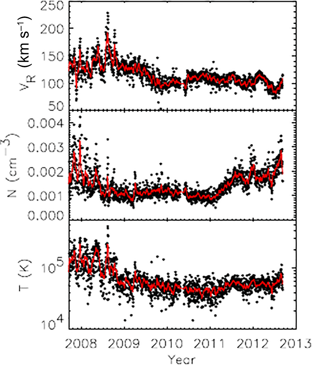
Figure 1Daily (points) and 11-day running averages (lines) of the radial speed, density, and temperature observed at V2. Taken from Richardson and Wang (2012).
In this volume a proper time τ is counted (i.e., the time of the comoving clock), and we want to describe the temperature change within the box as a function of τ. For an adequate estimate we use a simple thermodynamic transport equation describing the proton temperature as the result of charge-exchange-related energy exchanges between the plasma and the neutral gas in the following form:
with np≃const (see the assumption of incompressible heliosheath plasma flow as made in Fahr et al., 2016), nH≃const, kT≫kT0, and T(τ)∼O(105K) (see Richardson and Wang, 2012) denoting the actual, local ion temperature, T0 denoting the thermalized heliosheath pick-up ion temperature downstream of the shock, and denoting the temperature of the newly injected ions originating from the cold LISM H atoms (where U0 is the bulk speed of the proton fluid in the heliosheath). This equation can evidently be simplified to
and with leads to
yielding with σex=const
where January 2008, the date when Voyager 2 started moving within the heliosheath. Adopting a time period s, we find
assuming km s−1 and . This yields K. This estimate has to be compared with temperatures of about 40 000 K measured by Voyager 2 in 2011 and indicates that an essential part of the ion cooling may be ascribed to ongoing charge exchange reactions removing high-energy ions and replacing them by low-energetic ones.
Because the heliosheath plasma is convected along streamlines that originate at different points on the termination shock, it must be kept in mind that Voyager 2 crosses different streamlines (see Fig. 2) when moving through the inner heliosheath. On these different streamlines the solar wind evolves differently, as has been quantified in Fahr et al. (2016). Furthermore, we assumed that the locally prevailing temperature is a κ temperature Tκ resulting from an incompressible plasma flow:
In the following, after discussing the variation in κ and κ temperature along the Voyager 2 trajectory, we derive how the Maxwellian temperatures can be translated in κ temperatures.
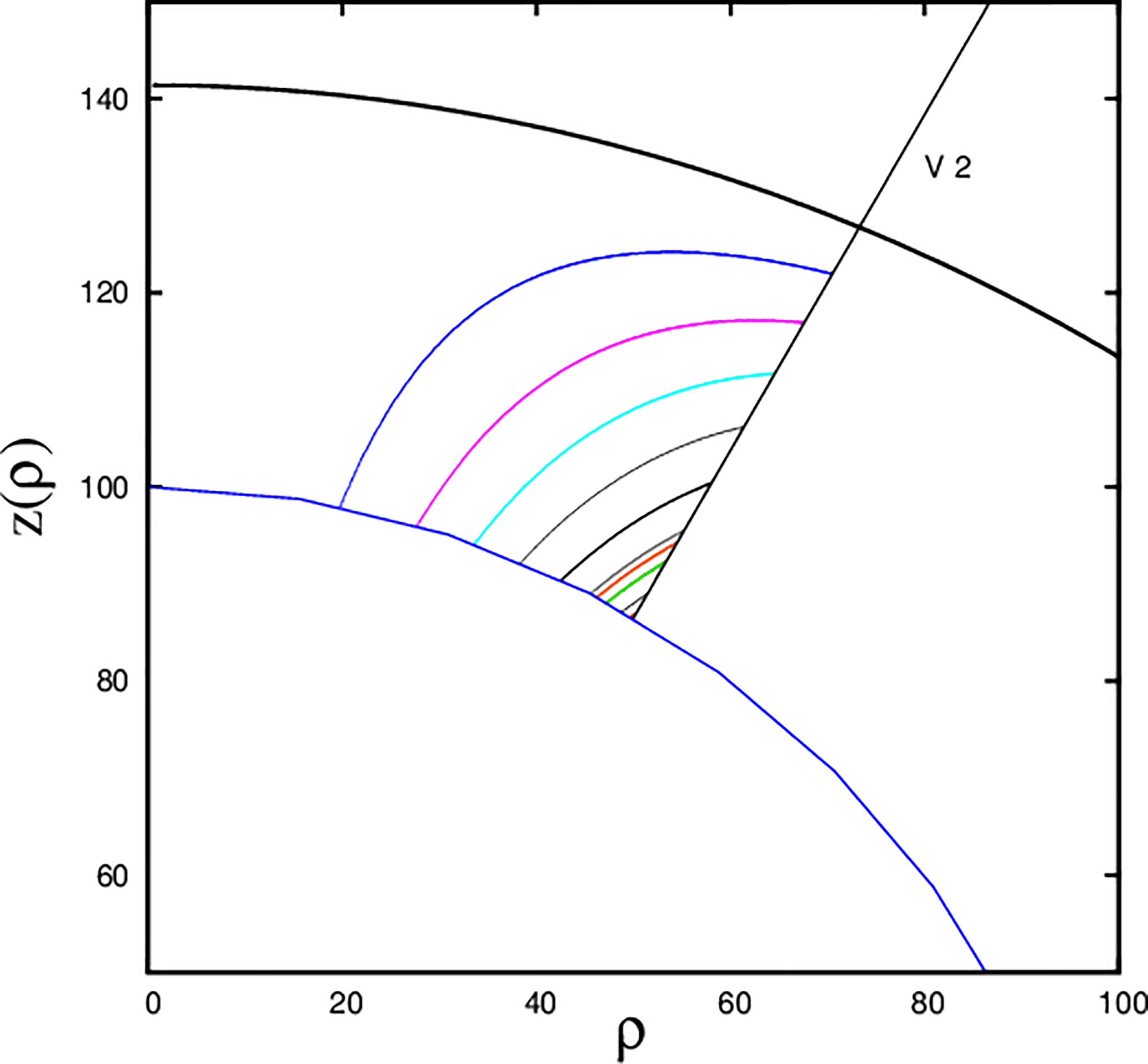
Figure 2Some streamlines originating at different points at the termination shock are shown with different colors. The Voyager 2 trajectory is the black straight line crossing the various streamlines on which the solar wind has evolved differently (Fahr et al., 2016).
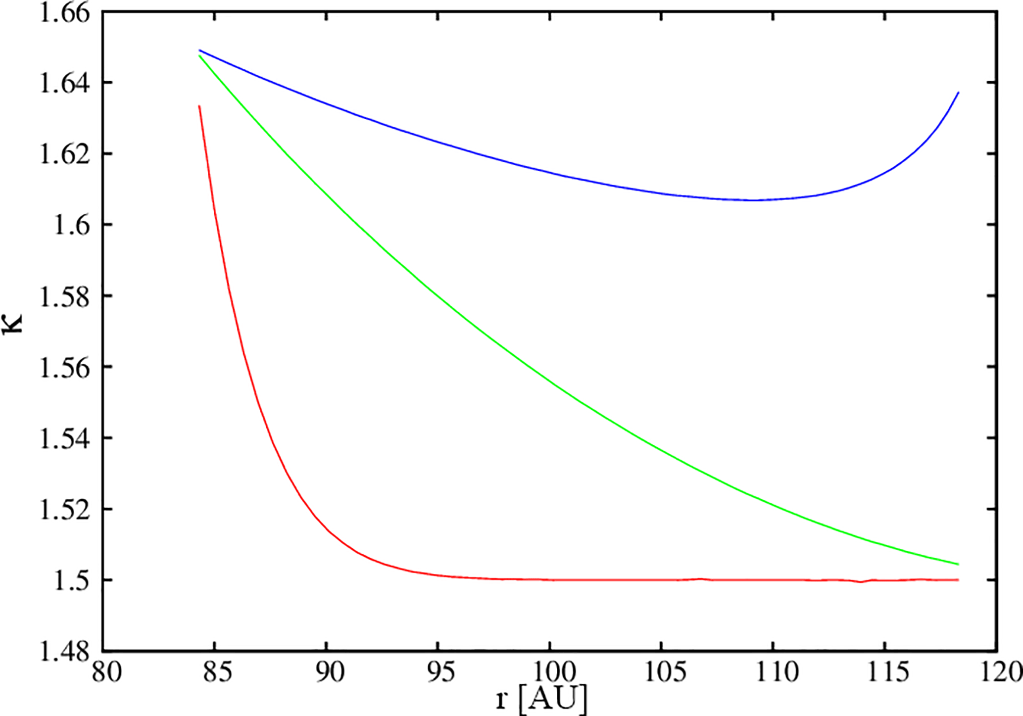
Figure 3κ evolution for three different momentum diffusion coefficients: (red, green, and blue curve, respectively) along the Voyager 2 trajectory. See Fahr et al. (2016) for details.
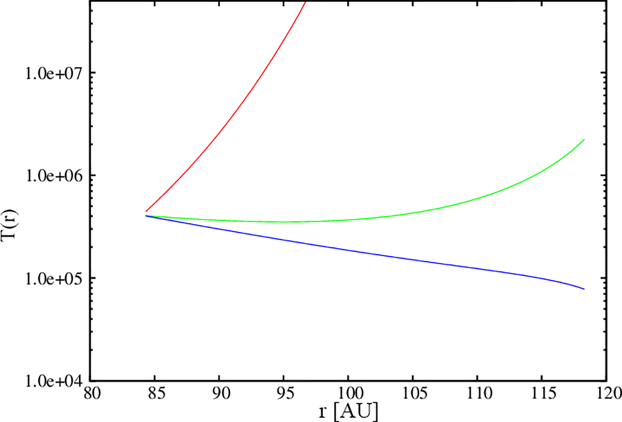
Figure 4The κ temperature derived from Eq. (9) of Fahr et al. (2016) using the results shown in Fig. 3

Figure 5Sketch of a realistic situation for fitting the data (histogram, i.e., currents in the instrument cups). The black line shows a shifted Maxwellian and three shifted κ distributions with κ=1.6 (red), κ=3 (blue), and κ=10 (green). The numbers on the x axis are the channel numbers, which can be translated to energy or velocity. The y axis is in arbitrary units. The distribution functions are multiplied with the velocity, which is approximately a representation of the currents; see Bridge et al. (1977).

Figure 6The truncated moments (a) and (b) for different κ values. The logarithmic x axis displays the speed normalized to 100 km s−1 and the y axis is in arbitrary units. See text for details. The dotted vertical line indicates a speed of roughly 200 km s−1, which is about the solar wind speed in the heliosheath. A speed about 30 units corresponds to that of protons as measured in the lowest-energy channel of the LECP instrument onboard Voyager.
In Fahr et al. (2016) we developed a numerical procedure to calculate the ion pressure evolution along arbitrarily selected flow lines of the heliosheath plasma flow on the basis of a pressure transport equation in which it was assumed that at each location in the plasma flow the underlying distribution function can be approximated by a κ distribution . This method allowed us to estimate the evolution of the κ parameter along each streamline.
In Fig. 3 we show how the κ parameter varies in turn along the Voyager 2 trajectory (displayed as heliocentric distance in AU). Depending on the magnitude of the velocity diffusion coefficient D0 (Fahr et al., 2016), one can see along the Voyager 2 trajectory different κ values (green, red, or blue curves). The more efficient the velocity diffusion process, the lower the resulting κ values at Voyager 2. Directly connected with these κ values are the associated κ temperatures Tκ along the Voyager 2 trajectory (see Eq. 11) as shown in Fig. 4.
We use the standard coordinate system for distribution functions, namely the space coordinates in the solar frame and the velocity coordinates in the rest frame (bulk frame) of the fluid. We assume isotropic distributions as defined in Sect. 1.1 above in each case.
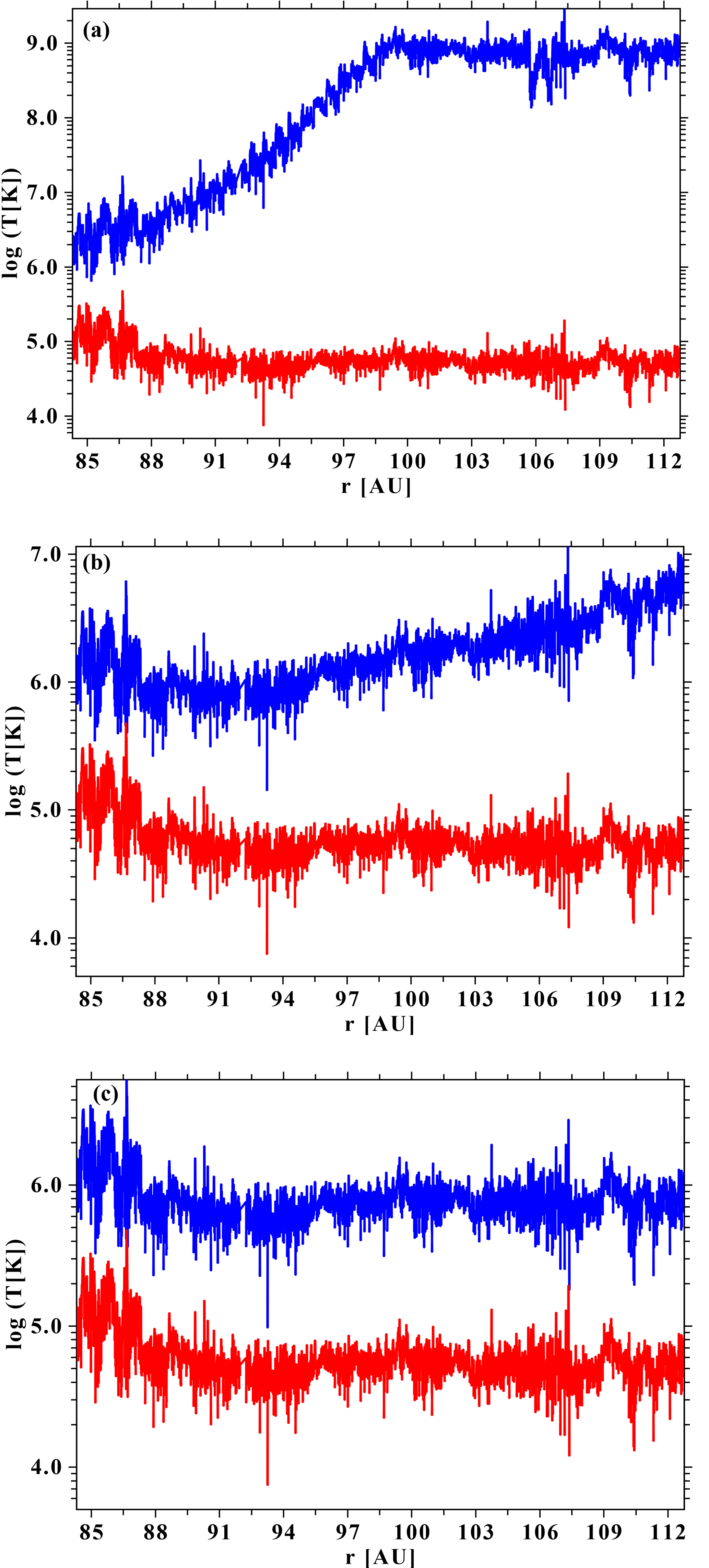
Figure 7The estimated κ temperature (blue lines) using Eq. (17) and the κ parameter along the Voyager 2 trajectory as calculated by Fahr et al. (2016). The lower red curves are the Voyager data form NSSDC (http://omniweb.gsfc.nasa.gov/coho/form/voyager2.html). From top to bottom (a–c), the diffusion coefficients as given in Fahr et al. (2016) change from , 10−9, 10−10 cm2 s−3, respectively.
5.1 The data fitting procedure
A problem now unavoidably arises when using observations like those from the plasma instrument onboard Voyager 2 (Richardson, 2008) with only a few data points in a limited energy range to fit a distribution function.
The physical parameters like density, temperature, and velocity are obtained from the currents of the different cups in the PLS instrument onboard Voyager 2. These currents correspond to a kinetic energy (momentum) from which the parameters are derived assuming a best-fit Maxwellian (Barnett, 1986; Richardson, 2008). Such a best fit is shown in Fig. 5 using data given by Richardson (2008), in which the black (step-like) lines show the measurements and the result of the best fit with a Maxwellian. We have also plotted results using κ distributions with different κ values. It can be seen that the representations by the alternative κ distributions give similar results in the measurement range but deviate from the Maxwellian fit at higher energies (channels). So, in the range not covered by data the tails of the distribution functions can contribute remarkably to the higher moments, especially to the pressure (temperature). Thus the latter can strongly differ from that obtained by using Maxwellians.
5.2 Truncated distribution functions
Based on the above discussion we only have available truncated distribution functions that have to deliver the fit. In the case of a Maxwellian this is not a problem. For the κ distribution, however, the core for different κ values can be fitted quite well, while the very different tails that are not taken into account into the fit imply that particles far off the core contribute remarkably to the temperature moments. It can be seen in Fig. 5 that the fits to the κ distribution can easily produce substantial differences in the expected values for different κ. This is shown in Fig. 6 in which we have plotted the truncated zeroth- and second-order moments normalized to the number density. That is,
It can be seen in the left panel of Fig. 6 that for different sets of (κ,Θ) for small normalized speed values, the different κ distribution zeroth-order moments are approximately the same, but strongly differ in the second-order moments for small κ ⪅ 2 above a truncation speed (see right panel), which is usually higher than the range covered by observations. These incomplete distribution functions are the true problem when interpreting observational data, while the problem faced by Nicolaou and Livadiotis (2016) considering complete (idealized) distribution functions appears more academic. Measured distributions are constrained by the instrument limitations, for instance given by the energy range detected by the instrument for which the highest-energy channel may define a truncation limit of the distribution function and its moments.
We have extended the range of the x axis to match the lowest channel of the LECP instrument onboard Voyager 2, which measures energetic protons in the energy range of ≈40 keV corresponding to roughly 3000 km s−1. It becomes obvious from Fig. 6 that these particles do not essentially contribute to the number density for different κ values, but they heavily influence the second-order moment (the pressure). Because the contribution of the high-energy particles to the number density is so small, it is not an easy task to determine the κ value. It will require more advanced models, which go far beyond the scope of this paper to determine the κ distribution from data of different instruments.
5.3 Analytic estimate of the κ distribution temperature
From the second moments we can find a relation between the pressures of a κ distribution Pκ and that of a Maxwellian Pm (see Eq. A10).
Now we can either calculate the Maxwellian pressure from the observed Maxwellian temperature Tm by using
with the Boltzmann constant k and comparing the pressure terms or, we define the κ temperature Tκ by using
and compare the “temperatures”. The result is the same, except for absolute numbers. With this definition we find
which is identical to Eq. (11).
Furthermore, because for κ→∞ the κ temperature must be equal to that of the Maxwellian, we find that vT=Θ and finally, since Θ is independent of κ,
depends only on κ and can be easily calculated from the Maxwellian temperature knowing the corresponding κ. Thus one can use the temperatures derived from a Maxwellian distribution and calculate from that the κ temperatures; κ and Θ can be estimated elsewhere, for instance by solving a kinetic transport equation as done in Fahr et al. (2016).
That also means that the presented temperatures derived with a Maxwellian as available from Omniweb (http://omniweb.gsfc.nasa.gov/coho/form/voyager2.html) must be taken with care because they should translate into κ distribution temperatures along the Voyager 2 trajectory through the inner heliosheath. With Eq. (17) this is an easy task knowing κ.
In Fig. 7 we have plotted the Voyager 2 temperature data between 84 and 112 AU, together with those obtained from the κ parameter of Fahr et al. (2016) using Eq. (17). In the left panel of Fig. 7 the κ parameter reaches the limiting value of 1.5, and to avoid numerical problems it was set to κ=1.5001 beyond r≈98 AU. Thus beyond 98 AU the model by Fahr et al. (2016) is not applicable for such high values of the diffusion coefficient ( cm2 s−1), while it can nicely explain the nonadiabatic behavior of the temperature between ≈88 and ≈98 AU.
This shows that the temperature highly depends on the underlying distribution function, and thus temperature data have to be taken with care because they can easily lead to erroneous interpretations of the data. This holds true in general.
The above study shows how Maxwellian temperatures derived from Voyager 2 measurements can easily be translated into corresponding κ temperatures. We have also shown (like Nicolaou and Livadiotis, 2016) that the temperature of a plasma highly depends on the underlying distribution function and differs from that obtained by a Maxwellian. This implies the need for knowledge of the underlying distribution function because otherwise the temperature is not well defined.
The recently presented study by Nicolaou and Livadiotis (2016) is not helpful in the “data-relevant” aspects discussed here because the authors compare moments calculated on the basis of κ or Maxwell distributions; however, they are taken from an infinite velocity range, while in reality data only support moments in a very limited velocity range. This is the important aspect that has to be taken seriously in these matters.
Nevertheless, after deriving a κ distribution from theoretical considerations it is an easy task to determine the corresponding κ temperature when a Maxwellian temperature is given. From IBEX observations (McComas et al., 2015a) it might be possible to obtain the κ value from which the temperature can be estimated. Note that previous attempts to do so (e.g., Livadiotis et al., 2011; Zirnstein and McComas, 2015) use a κ-independent temperature, which is a concept under debate (Lazar et al., 2016, 2017).
The procedure discussed in the present paper may not only be applied to spacecraft observations but also to all observations in which temperature is derived with the assumption that the underlying distribution function is a Maxwellian.
The Voyager data used for Fig. 7 can be accessed at http://omniweb.gsfc.nasa.gov/coho/form/voyager2.html (OMNIWeb, 2018).
From the moments of a distribution function the macroscopically observable quantities can be derived (for example, Goedbloed and Poedts, 2004, and many others). To calculate the moments one has to integrate the distribution function times some power α of the speed. For the Maxwell distribution the integrals are well known and can be found elsewhere (e.g., Gradshteyn and Ryzhik, 2007). For the κ distribution they can also be found in a more general form in Gradshteyn and Ryzhik (2007), Nr 3.251.2:
where Γ is the gamma function. With
we have the integral (Fahr et al., 2014)
and thus , where
is the normalization factor of the κ distribution defined in Eq. (1).
With the above integral we can thus easily calculate the following moments of the κ distribution of fκ and compare them to those for a Maxwell distribution fm.
In the comoving reference frame the first-order moment M1 vanishes. Furthermore, we assume that the stress tensor will be described by an isotropic pressure and thus the dyadic v⊗v can be contracted to a scalar M2 as . In addition we calculate the most probable speed by using
We find the following for the different moments.
The pressure ratio is
Finally, replacing the velocity in the fluid rest frame by that in the observer frame, which is where u is the fluid bulk velocity and w the thermal velocity, one easily finds that the zeroth moment remains, the first moment gives the bulk speed, and in the second moment the ram pressure appears as an additional term.
The authors declare that they have no conflict of interest.
The work of Hans Jörg Fahr and Klaus Scherer was partly carried out within the framework of
the bilateral BMBF–NRF project “Astrohel” (01DG15009) funded by
the Bundesministerium für Bildung und Forschung.
Responsibility for the contents of this work lies with the authors. Adama Sylla
acknowledges support via DFG project FI706/21-1. John D. Richardson was
supported under NASA contract 959203 from the Jet Propulsion
Laboratory to the Massachusetts Institute of Technology.
The topical editor, Margit Haberreiter, thanks two anonymous referees for help in evaluating this paper.
Barnett, A.: In situ measurements of the plasma bulk velocity near the Io flux tube, J. Geophys. Res.-Space, 91, 3011–3019, https://doi.org/10.1029/JA091iA03p03011, 1986. a
Bridge, H. S., Belcher, J. W., Butler, R. J., Lazarus, A. J., Mavretic, A. M., Sullivan, J. D., Siscoe, G. L., and Vasyliunas, V. M.: The plasma experiment on the 1977 Voyager mission, Space Sci. Rev., 21, 259–287, https://doi.org/10.1007/BF00211542, 1977. a, b
Chalov, S. V. and Fahr, H. J.: Phase space diffusion and anisotropic pick-up ion distributions in the solar wind: an injection study, Astron. Astrophys., 335, 746–756, 1998. a
Fahr, H. J.: Non-thermal solar wind heating by supra-thermal ions, Sol. Phys., 30, 193–206, 1973. a
Fahr, H.-J., and Siewert, M.: The multi-fluid pressures downstream of the solar wind termination shock, Astron. Astrophys., 558, A41, https://doi.org/10.1051/0004-6361/201322262, 2013. a
Fahr, H.-J., Fichtner, H., and Scherer, K.: On the radial evolution of κ distributions of pickup protons in the supersonic solar wind, J. Geophys. Res.-Space, 119, 7998–8005, https://doi.org/10.1002/2014JA020431, 2014. a, b
Fahr, H.-J., Sylla, A., Fichtner, H., and Scherer, K.: On the evolution of the κ distribution of protons in the inner heliosheath, J. Geophys. Res.-Space, 121, 8203–8214, https://doi.org/10.1002/2016JA022561, 2016. a, b, c, d, e, f, g, h, i, j, k, l
Fichtner, H., Sreenivasan, S. R., and Fahr, H. J.: Cosmic ray modulation and a non-spherical heliospheric shock., Astron. Astrophys, 308, 248–260, 1996. a
Fisk, L. A., Gloeckler, G., and Schwadron, N. A.: On theories for stochastic acceleration in the solar wind, Astrophys. J., 720, 533–540, https://doi.org/10.1088/0004-637X/720/1/533, 2010. a
Gloeckler, G.: Ubiquitous suprathermal tails on the solar wind and pickup ion distributions, in: Solar Wind Ten, edited by: Velli, M., Bruno, R., Malara, F., and Bucci, B., vol. 679 of American Institute of Physics Conference Series, 583–588, https://doi.org/10.1063/1.1618663, 2003. a
Goedbloed, J. P. H. and Poedts, S.: Principles of Magnetohydrodynamics, Cambridge University Press, Cambridge, UK, 2004. a
Gradshteyn, I. S. and Ryzhik, I. M.: Table of Integrals, Series, and Products, Elsevier/Academic Press, Amsterdam, 2007. a, b
Heerikhuisen, J., Pogorelov, N. V., Florinski, V., Zank, G. P., and le Roux, J. A.: The effects of a κ-distribution in the heliosheath on the global heliosphere and ENA flux at 1 AU, Astrophys. J., 682, 679–689, https://doi.org/10.1086/588248, 2008. a
Hill, M. E., Haggerty, D. K., McNutt, R. L., and Paranicas, C. P.: Energetic particle evidence for magnetic filaments in Jupiter's magnetotail, J. Geophys. Res.-Space, 114, A11201, https://doi.org/10.1029/2009JA014374, 2009. a
Holzer, T. E. and Leer, E.: Solar wind heating beyond 1 AU, Astrophys. Space Sci., 24, 335–347, 1973. a
Isenberg, P. A.: Interstellar pickup ions: not just theory anymore, Rev. Geophys., 33, 623–627, https://doi.org/10.1029/95RG00553, 1995. a
Lazar, M., Poedts, S., and Fichtner, H.: Destabilizing effects of the suprathermal populations in the solar wind, Astron. Astrophys., 582, A124, https://doi.org/10.1051/0004-6361/201526509, 2015. a
Lazar, M., Fichtner, H., and Yoon, P. H.: On the interpretation and applicability of κ-distributions, Astron. Astrophys., 589, A39, https://doi.org/10.1051/0004-6361/201527593, 2016. a, b
Lazar, M., Pierrard, V., Shaaban, S. M., Fichtner, H., and Poedts, S.: Dual Maxwellian–Kappa modeling of the solar wind electrons: new clues on the temperature of Kappa populations, Astron. Astrophys., 602, A44, https://doi.org/10.1051/0004-6361/201630194, 2017. a
Livadiotis, G. and McComas, D. J.: Understanding kappa distributions: a toolbox for space science and astrophysics, Space Sci. Rev., 175, 183–214, https://doi.org/10.1007/s11214-013-9982-9, 2013. a
Livadiotis, G., McComas, D. J., Dayeh, M. A., Funsten, H. O., and Schwadron, N. A.: First sky map of the inner heliosheath temperature using IBEX spectra, Astrophys. J., 734, 1, https://doi.org/10.1088/0004-637X/734/1/1, 2011. a
McComas, D. J., Bzowski, M., Frisch, P., Fuselier, S. A., Kubiak, M. A., Kucharek, H., Leonard, T., Möbius, E., Schwadron, N. A., Sokół, J. M., Swaczyna, P., and Witte, M.: Warmer local interstellar medium: a possible resolution of the Ulysses-IBEX Enigma, Astrophys. J., 801, 28, https://doi.org/10.1088/0004-637X/801/1/28, 2015a. a
McComas, D. J., Bzowski, M., Fuselier, S. A., Frisch, P. C., Galli, A., Izmodenov, V. V., Katushkina, O. A., Kubiak, M. A., Lee, M. A., Leonard, T. W., Möbius, E., Park, J., Schwadron, N. A., Sokół, J. M., Swaczyna, P., Wood, B. E., and Wurz, P.: Local interstellar medium: six years of direct sampling by IBEX, Astrophys. Supp., 220, 22, https://doi.org/10.1088/0067-0049/220/2/22, 2015b. a
Nicolaou, G. and Livadiotis, G.: Misestimation of temperature when applying Maxwellian distributions to space plasmas described by kappa distributions, Astrophys. Space Sci., 361, 359, https://doi.org/10.1007/s10509-016-2949-z, 2016. a, b, c, d, e
OMNIWeb: Voyager data, available at: http://omniweb.gsfc.nasa.gov/coho/form/voyager2.html, last access: 10 January 2018.
Pierrard, V. and Lazar, M.: Kappa distributions: theory and applications in space plasmas, Sol. Phys., 267, 153–174, https://doi.org/10.1007/s11207-010-9640-2, 2010. a
Pogorelov, N. V., Bedford, M. C., Kryukov, I. A., and Zank, G. P.: Pickup ion effect of the solar wind interaction with the local interstellar medium, J. Phys. Conf. Ser., 767, 012020, https://doi.org/10.1088/1742-6596/767/1/012020, 2016. a
Richardson, J. D.: Plasma temperature distributions in the heliosheath, Geophys. Res. Lett., 35, L23104, https://doi.org/10.1029/2008GL036168, 2008. a, b, c
Richardson, J. D. and Wang, C.: Voyager 2 observes a large density increase in the heliosheath, Astrophys. Lett., 759, L19, https://doi.org/10.1088/2041-8205/759/1/L19, 2012. a, b, c, d
Schwadron, N. A., Fisk, L. A., and Gloeckler, G.: Statistical acceleration of interstellar pick-up ions in co-rotating interaction regions, Geophys. Res. Lett., 23, 2871–2874, https://doi.org/10.1029/96GL02833, 1996. a
Siewert, M. and Fahr, H.-J.: Full Boltzmann–kinetical treatment of an ion plasma crossing an MHD shock: parallel and non-parallel cases, Astron. Astrophys., 471, 7–15, https://doi.org/10.1051/0004-6361:20077413, 2007. a
Vasyliunas, V. M. and Siscoe, G. L.: On the flux and the energy spectrum of interstellar ions in the solar system, J. Geophys. Res., 81, 1247–1252, 1976. a
Zirnstein, E. J. and McComas, D. J.: Using kappa functions to characterize outer heliosphere proton distributions in the presence of charge-exchange, Astrophys. J., 815, 31, https://doi.org/10.1088/0004-637X/815/1/31, 2015. a
- Abstract
- Introduction
- κ distributions
- Maxwellian temperatures along the Voyager 2 trajectory
- Heliosheath plasma along the Voyager 2 trajectory
- κ temperatures along the Voyager 2 trajectory
- Conclusions
- Data availability
- Appendix A: Moments of the distribution function
- Competing interests
- Acknowledgements
- References