the Creative Commons Attribution 4.0 License.
the Creative Commons Attribution 4.0 License.
 | 05 Mar 2018
Case study of mesospheric front dissipation observed over the northeast of Brazil
Amauri Fragoso Medeiros
Cristiano Max Wrasse
Joaquim Fechine
Hisao Takahashi
José Valentin Bageston
Ana Roberta Paulino
Ricardo Arlen Buriti
On 3 October 2005 a mesospheric front was observed over São João do Cariri (7.4∘ S, 36.5∘ W). This front propagated to the northeast and appeared in the airglow images on the west side of the observatory. By about 1.5 h later, it dissipated completely when the front crossed the local zenith. Ahead of the front, several ripple structures appeared during the dissipative process of the front. Using coincident temperature profile from the TIMED/SABER satellite and wind profiles from a meteor radar at São João do Cariri, the background of the atmosphere was investigated in detail. On the one hand, it was noted that a strong vertical wind shear in the propagation direction of the front produced by a semidiunal thermal tide was mainly responsible for the formation of duct (Doppler duct), in which the front propagated up to the zenith of the images. On the other hand, the evolution of the Richardson number as well as the appearance of ripples ahead of the main front suggested that a presence of instability in the airglow layer that did not allow the propagation of the front to the other side of the local zenith.
Keywords. Atmospheric composition and structure (airglow and aurora) – meteorology and atmospheric dynamics (middle atmosphere dynamics; waves and tides)
- Article
(2115 KB) - Full-text XML
-
Supplement
(2969 KB) - BibTeX
- EndNote


Mesospheric fronts have recently been studied around the world (e.g., Isler et al., 1997; Brown et al., 2004; She et al., 2004; Smith et al., 2005; Medeiros et al., 2005, 2016; Fechine et al., 2005, 2009; Nielsen et al., 2006; Narayanan et al., 2009, 2012; Yue et al., 2010; Bageston et al., 2011a; Dalin et al., 2013). This kind of gravity wave can propagate horizontally for long distances since they are generally trapped in ducts, where the dissipation of energy is neglected (e.g., Dewan and Picard, 2001). Consequently, they are an efficient mechanism for transferring energy and momentum over long distances in the atmosphere. Furthermore, along the path in the atmosphere, they can interact with other gravity waves and the background atmosphere producing complex dynamical structures, like dynamical and convective instabilities (e.g., Fritts and Rastogi, 1985; Fritts et al., 1994). According to Dewan and Picard (1998), mesospheric fronts can also be classified as a mesospheric bores and mesospheric walls, depending on the physical structure.
Ducts are the main requirement for the existence and propagation of mesospheric fronts. Ducts can be thermal (e.g., Meriwether et al., 1998), Doppler (e.g., Fechine et al., 2009) and dual ducts (e.g., Bageston et al., 2011a; Carvalho et al., 2017). Thermal ducts are created by a discontinuity in the temperature lapse rate. Doppler ducts appear whenever the wind shear is primarily responsible for its formation. Alternatively, when both wind and temperature have significant contributions, a dual duct is formed.
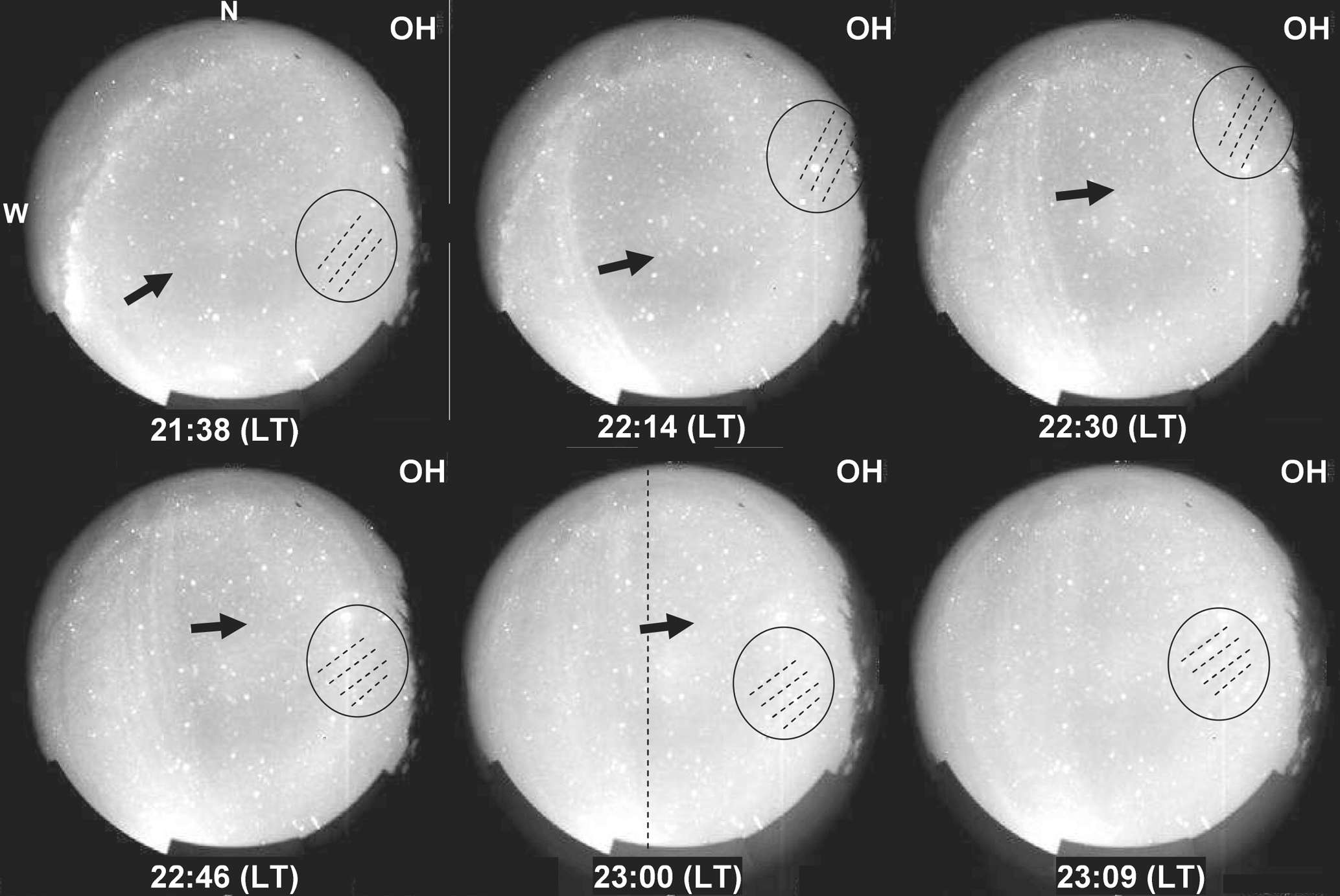
Figure 1Successive images of the OH airglow emission showing the mesospheric front observed on the 3 October 2005 over São João do Cariri. The arrows indicate the propagation direction of the wave front. The circles indicate the ripple occurrence (dashed lines) and the vertical dashed line indicates the region where the front disappeared. See the movie in the Supplement for further details about the propagation of the front and the presence of ripples (https://doi.org/10.5446/35010).
Airglow imaging is the most important technique that has been used to observe mesospheric fronts. The first report was done during the ALOHA campaign (Taylor et al., 1995). In the airglow images, mesospheric fronts are observed with a long extension, i.e., over 500 km, and they generally cover the whole image diameter. Another advantage of airglow imaging is that there are multiple emissions from the mesosphere and lower thermosphere (MLT) region, which comes from a common volume with peaks at different altitudes. Then, the airglow images can be used to study the pattern of the front at different altitudes and the observed patters can be compared to theoretical models (e.g., Dewan and Picard, 1998). Thus, it is possible to infer the altitude of the duct in the MLT. In the case of an undular bore, airglow images can also be used to estimate the horizontal parameters (period, wavelength and propagation direction) of the trailing waves. Airglow images are useful to observe the interaction of the mesospheric front with other gravity wave types as well.
Mesospheric inversion layers (MILs) have been identified as an important factor for the formation of mesospheric ducts (e.g., Leblanc and Hauchecorne, 1997; Meriwether et al., 1998; Liu and Meriwether, 2004; Fechine et al., 2008; Ramesh and Sridharan, 2012). Whenever MILs are created, one can observe inversions in the vertical temperature profiles of the background mesosphere. The typical lapse rate in the mesosphere is positive and the generation of MILs happen when the lapse rate becomes negative for a short range of altitudes.
The biggest challenge in the study of mesospheric fronts is the knowledge of the background atmospheric conditions that are creating the ducts. In general, airglow observations with background conditions are rare (e.g., Sivakandan et al., 2015). In the present work, dissipation of a mesospheric front observed on 3 October 2005 over São João do Cariri (7.4∘ S, 36.5∘ W) is studied using coincident winds from a meteor radar and temperature profiles from the Sounding of the Atmosphere using Broadband Emission Radiometer (SABER) instrument onboard the Thermosphere-Ionosphere-Mesosphere Dynamics (TIMED) satellite. Using these collocated measurements, it was possible to investigate the temporal evolution of the background atmosphere and evaluate the contribution of the wind and temperature for the disappearance of the front.
An all-sky airglow imager operated in São João do Cariri from 2000 to 2010 using five interference filters, which observed OH NIR, OI 557.7 nm (OI5577), O2 (0, 1), OI 630.0 nm (OI6300) airglow emissions and a background. This system used a charge-coupled device (CCD) of 6.45 cm2 of area, a 1024×1024 back-illuminated array of 14-bit pixels. Moreover, this CCD imager has a high quantum efficiency, low dark current (0.5 electrons pixel−1 s−1), low readout noise (15 electrons rms) and high linearity (0.05 %). It also uses a fisheye lens (f/4), which enables it to observe airglow emissions of the whole sky with an exposure time of typically 15 s for the OH emission and 90 s for the other emissions. The CCD camera was manufactured by the Keo Scientific Ltd. and the model of the CCD is CH350, number A99F2107.
Figure 1 shows a sequence of OH airglow images on 3 October 2005 over São João do Cariri from 21:38 to 23:09 LT (local time). One can see in these images a front followed by five bright crests and there are also ripple structures ahead of the front. The ripple structures are denoted by dashed lines inside the black circle plotted on each image in order to easily identify their position, since it difficult to identify such structures in still images. Around 23:00 LT the mesospheric front dissipates and the position in the image where the front disappeared is marked with a vertical dashed line. See the movie in the Supplement for further details about the propagation of the front and the presence of ripples (https://doi.org/10.5446/35010).
The mesospheric front was observed for approximately 150 min in the OH airglow images and it was seen very clearly for more than 30 min (22:14–22:46 LT). This event was also observed in the OI5577 (not shown here) with the complementary bright-dark effect (Medeiros et al., 2005). Along the passage of the front in the images, the trailing wave was enhanced with several wave crests added behind the main front. However, around 23:00 LT the wave starts to fade and after 23:30 LT the whole mesospheric front disappeared completely near the zenith. In addition, ripple structures are present in the images, mainly after about 23:00 LT in the eastern part. These ripples are denoted by small dashed lines inside the circles in Fig. 1 (second row of images) and they could be associated with the dissipation of the main front. The presence of ripples ahead of the mesospheric front is indicative of the instability of the atmosphere generated by the dissipation of larger waves (e.g., Carvalho et al., 2017; Li et al., 2017).
These observations suggest that there must be different atmospheric conditions during the night, which could be spatially marked by the vertical dashed line in Fig. 1, i.e., the front has conditions to propagate in the MLT before reaching this point.
Using two-dimensional spectral analysis in a sequence of images (Garcia et al., 1997; Wrasse et al., 2006), parameters of the trailing waves behind the front were calculated. The propagation direction was 58∘ from the north with an observed phase speed of 27 m s−1 (intrinsic velocity of 36.5 m s−1), observed period of ∼12 min and horizontal wavelength of 27 km. In order to calculate the intrinsic parameters, horizontal winds from a meteor radar deployed at São João do Cariri were used.
The meteor radar is composed of five receiver Yagi antennas, one transmitter Yagi antenna, a transmitter and a receiving module. The system operates at 35.24 MHz and transmits 2144 pulses per second. The meteor radar collects data continuously by transmitting pulses of electromagnetic waves and detecting reflected echoes by its receiving system. The echoes come from the MLT region (80–100 km height) and bring information about the neutral wind from that region. In this work, meteor echoes within 4 km thickness were used to calculate the wind centered at 81, 84, 87, 90, 93, 96 and 99 km heights. Further details about the meteor wind can be found in Paulino et al. (2015).
Considering the characteristics of the front, i.e., (i) the presence of an extended front, (ii) the presence of some trailing waves behind the front and (iii) the front propagating into a duct, and based on the criteria described by Dewan and Picard (1998), this front can be classified as a mesospheric bore. Several works have used these characteristics to distinguish bores from other mesospheric front types (e.g., Medeiros et al., 2001, 2005, 2016; Smith et al., 2003, 2005; Brown et al., 2004; She et al., 2004; Fechine et al., 2005; Narayanan et al., 2009, 2012; Yue et al., 2010; Bageston et al., 2011a, b; Suzuki et al., 2013).
Characterization of the duct was done using vertical profiles of wind and temperature and further details on the duct will be discussed later in Sect. 3. Temperature profiles were obtained from the SABER instrument, which is onboard the TIMED spacecraft. This spacecraft is almost sun-synchronous and precesses to cover 24 h and a 60-day yaw period. The TIMED satellite has an apogee of about 650 km and an inclination of 73∘. The SABER instrument retrieves temperature in the MLT region using non-local thermodynamic equilibrium (Mertens et al., 2001, 2004). Mertens et al. (2009) published a detailed study about the SABER temperatures and uncertainties. The volumetric emission rate (VER) of the OH airglow emission measured by the SABER has also been used in this work in order to identify the height of the OH emission layer.
In order to investigate the mesospheric environment on the night of the event, simultaneous measurements of winds, obtained by meteor radar, OH VER and temperature profiles obtained by the TIMED/SABER satellite (Mertens et al., 2004, 2009) were used. Figure 2 shows the profiles of (a) kinetic and potential temperatures, (b) square of the Brünt–Väisälä frequency, (c) horizontal wind in the propagation direction of the wave, (d) square vertical wavenumber and (e) VER profile of OH at 1.6 µm.
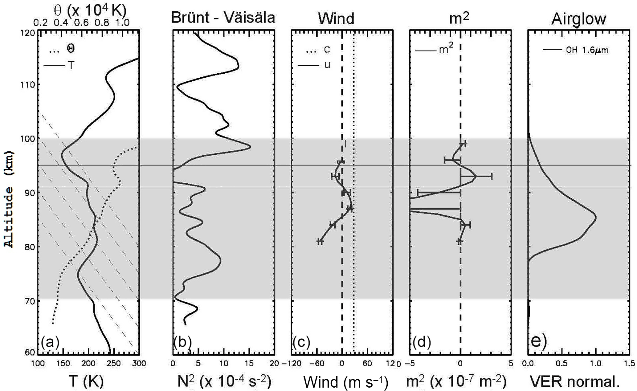
Figure 2(a) Kinetic temperature profile (solid line) obtained by the TIMED/SABER satellite on 3 October 2005 over São João do Cariri and potential temperature profile (dotted line). The dashed lines represent the adiabatic lapse rates. (b) Square of the Brünt–Väisälä frequency profile. (c) Wind profile in the same propagation direction as the wave front measured at 21:00 LT by a meteor radar (solid line). The dotted line represents the observed wave velocity (∼27 m s−1). (d) Vertical squared wavenumber (m2; solid line). (e) Normalized volumetric emission rate (VER) profiles of the OH at 1.6 µm (solid line) measured by the TIMED/SABER satellite. The horizontal solid lines in all charts show the top and bottom of the duct and a shaded box emphasizes the altitude range from 70 to 100 km.
In order to discuss the static stability of the mesosphere on the night of the event, the potential temperature profile (dotted line) in Fig. 2a was calculated from pressure and temperature data obtained by the TIMED/SABER instrument at 2.9∘ N, 41.9∘ W and 21:58 LT on 3 October 2005. From Fig. 2a and b, one can see that, in general, the mesosphere was stable, presenting only narrow regions of instability at approximately 70, 93 and 110 km where N2 was near zero, and near 93±1 km the duct region was especially unstable (N2<0 and decreasing in potential temperature) probably caused by the bore propagation and dissipation near the zenith. But, on the other hand, the increasing in the potential temperature between 75 and 91 km shows the stability of this portion of the mesosphere and also the region above 95 km height. The dashed line represents the adiabatic lapse rate, i.e., ∼9.8 K km−1.
Also, a mesospheric inversion layer (MIL) was observed between 75 and 82 km with an amplitude of ∼37 K. Above the peak of the MIL, the temperature started to decrease with a rate larger than the adiabatic lapse rate. The thickness of the MIL was in agreement with previous observations in the region of São João do Cariri (Fechine et al., 2008), but this inversion is not sharp enough and probably will have a slight contribution to the duct formation compared to the wind contribution (see discussion later).
Figure 2c shows the wind profile (solid line) in the propagation direction of the wave front and the observed phase velocity of the mesospheric bore (c ≅27.5 m s−1) is denoted by the vertical dotted line, while the vertical dashed line at zero is presented for reference to the wind variation (u). The original wind data have a temporal resolution of 1 hour. The wind data were smoothed in 3 h and vertically interpolated for every kilometer. One can see in Fig. 2c that the wind blows in the opposite direction of the front below 85 km height. Above this height, the wind blows in the same direction of the front and between 87 and 90 km the wind velocity approaches the phase speed of the front, which is compatible with the presence of a critical level. Above 91 km the wind turns to change its direction, blowing in the opposite direction of the wave front, and around 96 km the wind becomes negligible.
Figure 2d shows the vertical wavelength (dotted line) and square wavenumber (solid line) profiles calculated for the trailing waves behind the mesospheric front. The m2 parameter was obtained by using the Taylor–Goldstein dispersion relation for gravity waves:
where, m is the vertical wavenumber, N2 is the square of the Brünt–Väisälä frequency, is the wind in the direction of wave propagation, c is the phase velocity of the wave and kh is the horizontal wave number.
The dispersion relation given in Eq. (1) is valid for gravity waves propagating in an environment where the effects of wind shear and temperature gradients can not be neglected (e.g., Chimonas and Hines, 1986; Isler et al., 1997). Two ducts can be observed in Fig. 2d, one between 82 and 85 km and another from 91 to 95 km height, which were candidates to support the propagation of the observed bore.
The first duct was mainly created by the wind gradient and the m2 was close to zero suggesting that the propagation of the bore was not efficient into this duct. On the other hand, the upper duct, between 91 and 95 km, occurred when it was observed at a minimum of the wind and had larger positive values for m2, which is more efficient for the canalization of the front.
Table 1Physical parameters of the trail front observed within the duct of the mesospheric front on 3 October 2005.
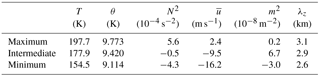
Figure 2e shows the normalized VER profile of the OH airglow emission from TIMED/SABER at 1.6 µm (solid line). Note that the upper duct (centered at 93 km) was quite above the peak of the OH emission (∼86 km) and slightly above of the peak of the OI5577 emission, which is typically around 96 km, and the duct region (between the horizontal solid lines) contains ∼11 % of the OH emission. As the front appeared bright in the OH and dark in the OI5577, the waves appear faint in the OH airglow images. It should be noted that a complementarity effect in this case study was observed that is in agreement with the bore model proposed by Dewan and Picard (1998) and also described by Medeiros et al. (2005).
The physical parameters for the trail front within the duct were calculated and are summarized in Table 1.
Earlier works have pointed out different types of ducts that support the propagation of mesospheric fronts. When the vertical profile of temperature is more important to the formation of the duct and there is a discontinuity in the temperature lapse rate, it is named a thermal duct (e.g., Bageston et al., 2011b). Doppler ducts occur wherever the gradient of the wind is predominant in its formation. Lastly, if both terms are important, the duct is termed as dual (e.g., Bageston et al., 2011a; Narayanan et al., 2012). Based on this, it is mandatory to investigate the contribution of each term of the dispersion relation in order to infer the nature of the duct where the mesospheric front was propagating.
By analyzing the terms of Eq. (1) in Fig. 2, combined with the wind variation and intensities in Fig. 3, it is feasible that the second derivative of the wind dominates the formation of the duct as compared to the contribution of the temperature, since the strongest inversion layer (from ∼75 to 80 km) is far below the main duct. So, in this case it can be suggested that the mesospheric front was propagating horizontally in a Doppler duct. Figure 3 shows contours of zonal and meridional winds measured with a meteor radar from 12:00 LT on 3 October to 12:00 LT on 4 October 2005 over São João do Cariri. The meridional and zonal wind structure showed that from 21:00 to 23:30 LT a wind shear was present in both meridional and zonal components of the wind. This wind shear was produced primarily due to the strength of the semidiurnal thermal tide (more evident in the zonal wind component) in the MLT on the observed night. The semidiurnal tide enhanced the mesospheric zonal wind, primarily in the high level of the MLT region. Further details on the contribution of the semidiurnal thermal tide in the winds over São João do Cariri can be found in the work of Lima et al. (2007).
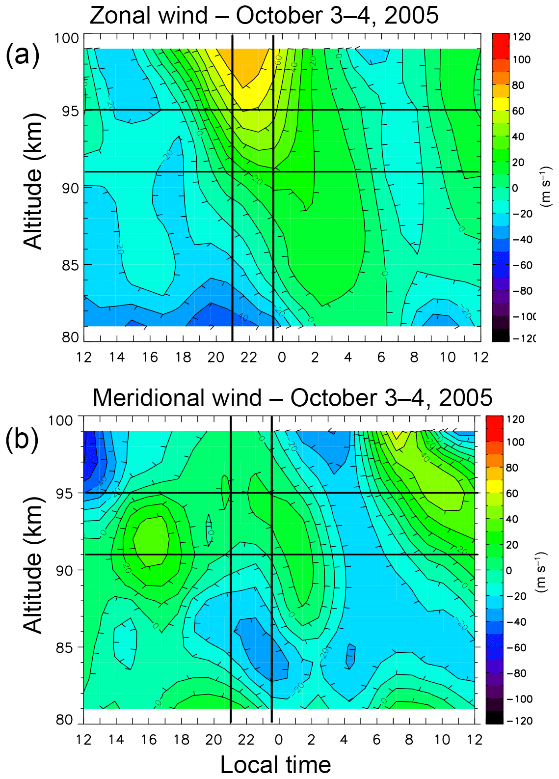
Figure 3Contours of (a) zonal wind and (b) meridional wind measured by a meteor radar from 12:00 LT on 3 October to 12:00 LT on 4 October 2005 over São João do Cariri. The vertical solid lines indicate the time window of observation of the wave front and the horizontal solid lines delimit the top and bottom of the duct shown in Fig 2.
Figure 4a shows the wind in the propagation direction of the front and it is quite similar to the zonal wind because the front was propagating almost northeastward. The wind in the direction of the front was ∼10 m s−1 weaker than the zonal component of the wind. The wind changed propagation direction above 89 km, which corresponds to the strong wind shear shown in Fig. 4b. It is important to note that this strong wind shear coincides to the time of propagation of the mesospheric front and it was caused mainly by the semidiurnal thermal tide.
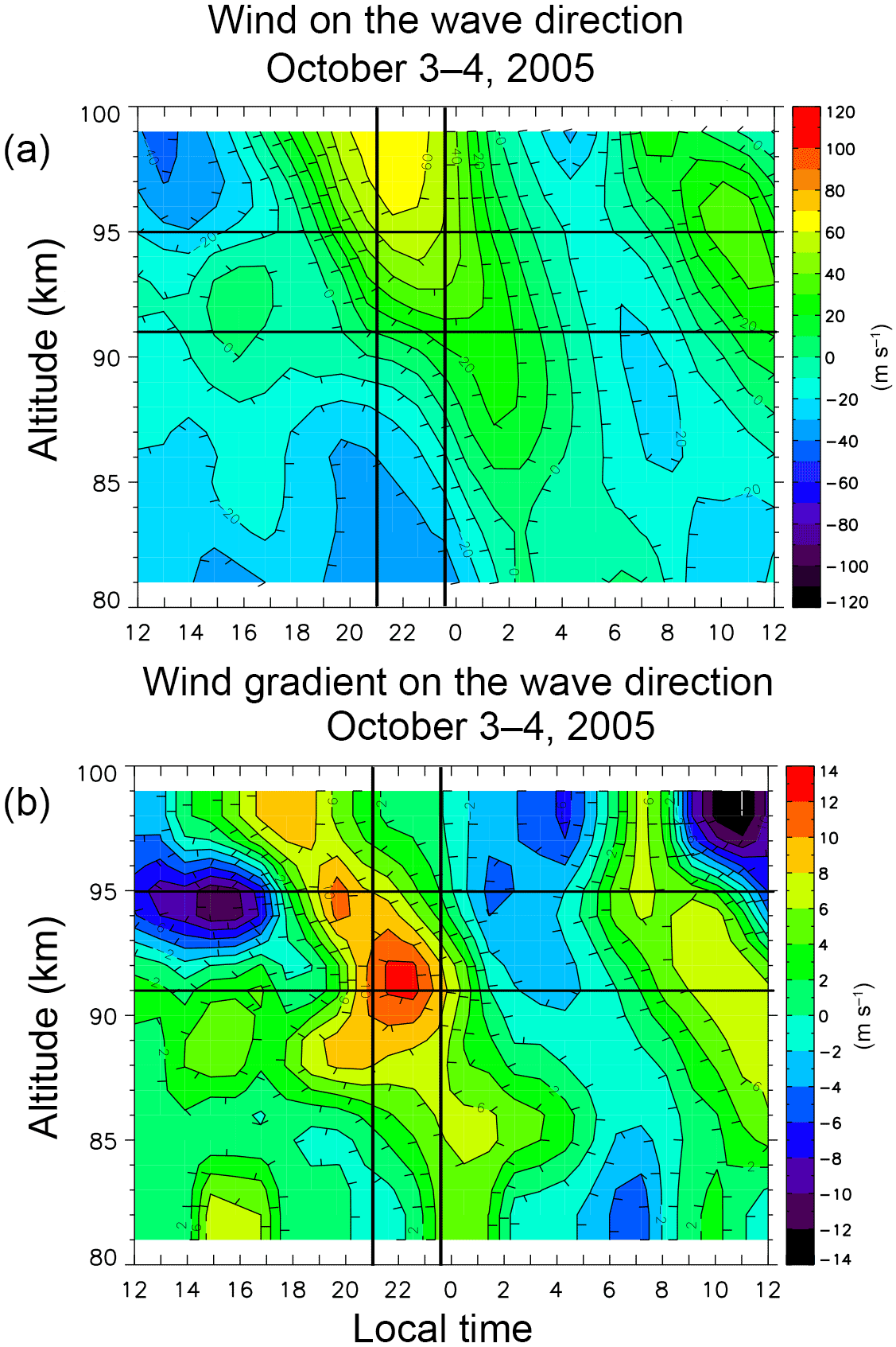
Figure 4Contourd of (a) wind (b) wind gradient measured in the direction of wave propagation with the meteor radar from 12:00 LT 3 October to 12:00 LT 4 October 2005 over São João do Cariri. The vertical solid lines indicate the observation time of the wave front and the horizontal solid lines delimit the top and bottom of the duct shown in Fig. 2.
The mesospheric front started to dissipate by about 22:45 LT (see images in the lower part of Fig. 1 and movie in the Supplement) and it disappeared completely at ∼23:30 LT when the front was near the local zenith. It can be considered that the dissipation of the mesospheric front associated with the region of instability (91–95 km height), which would have been caused by the intense wind shear at the heights of the duct occurrence during the period of propagation of the bore from the west to zenith. This hypothesis agrees with SABER measurements that showed an atmospheric instability around 93 km, as it can be noticed by the negative values of the Richardson number and a decrease in the potential temperature inside of the duct (Fig. 2a and b). These results also agree with previous works on atmospheric coupling and instability in the MLT region (Li et al., 2009; Cai et al., 2014).
An increase in the wind shear around 93 km, as can be seen in Fig. 3b, simultaneously with a decrease in the static stability is characterized as an ideal mechanism for the generation of dynamic instabilities in the atmosphere, as presented and discussed by Hecht (2004) and Hecht et al. (2014). The parameter that define this kind of instability is the Richardson number (Beer, 1974):
In fact, between 92 and 94 km Richardson numbers were negative, resulting in static instability, and this explains the fact that the mesospheric front and the trailing waves disappeared quickly at about 23:30 LT. However, the determination of the Richardson number can be ambiguous due to the ambiguity of the vertical gradient of the temperature and wind. Thus, in the present case, we can have a contribution of convective instability as well.
Another fact that supports the hypothesis of an unstable atmosphere between the zenith and the east of the observatory was the observation of ripples during the propagation of the bore from the west to the zenith and also after its disappearance. Ripples occurring after the vanishing of a mesospheric front was also observed in previous works (e.g., She et al., 2004; F. Li et al., 2005; T. Li et al., 2005; Hecht et al., 2005). In the present work, the destruction of the trailing waves associated with a mesospheric front could be indicative of a transition from an undular to a turbulent bore, as predicted by the model of Dewan and Picard (1998) and observed by Liu and Hagan (1998), although evidence of a turbulent bore could not be observed from the images. She et al. (2004) showed that in the moment of the transition from an undular to a turbulent bore, the Richardson number inside of duct was smaller than 0.25. In other words, the bore was likely subjected to a process of dynamic instability, but a contribution of convective instability can not be neglected at all. She et al. (2004) also observed the occurrence of ripples in the airglow images corroborating the hypothesis of the instability. So, the observations of She et al. (2004) support our hypothesis that the mesospheric bore observed on 3 October 2005 was destroyed by a process of instability in the atmosphere that was increasing during the propagation of the bore during the night at heights of about 90–95 km.
There is also another possibility to explain the vanishing of the bore, which consist of the duct conditions not holding after 23:00 LT. From Fig. 4b, one can see that the vertical gradient of the wind started to decrease, even before 23:00 LT. This can cause the disappearance of the duct conditions and the annihilation of the duct for the propagation of the bore. In this case, the bore could propagate either upward or downward and leave the airglow layers. Unfortunately, the images of OI5577 could not support this hypothesis.
On 3 October 2005, the propagation and dissipation of a mesospheric front was observed in the OH and OI5577 (not shown here) emission layers over São João do Cariri. The main results of this work are the following:
-
The presence of a duct below the peak of the OI5577 emission layer and above the peak of the OH layer making the mesospheric front to be dark in the OI5577 images and bright in the OH images (white front shown here).
-
This complementary bright-dark effect is predicted by the Dewan and Picard (1998) model due to its location in the MLT above the peak of the OH emission layer.
-
A strong and variable wind profile suggested a Doppler duct was caused mainly due to the strength of the semidiurnal tide, which supported the propagation of the mesospheric front over São João of Cariri.
-
One likely reason for the dissipation of the mesospheric bore was different conditions of propagation during the night. The presence of ripples in the eastern part of the images suggested instability in the atmosphere that can be generated by the dissipation of the front.
-
The increase in the wind shear can be the main mechanism that generates instabilities that could mainly contribute to the destruction of the bore near the zenith of São João do Cariri at the MLT region (90–95 km).
Airglow images for 3 October 2005 over São João of Cariri can be requested directly by e-mail to Amauri Medeiros (afragoso@df.ufcg.edu.br). SABER measurements are available online. Please contact Ricardo Buriti (rburiti@df.ufcg.edu.br) in order to request the meteor radar measurements for São João of Cariri.
The supplement related to this article is available online at: https://doi.org/10.5194/angeo-36-311-2018-supplement.
AFM has supervised the work and written most parts of the manuscript. IP and ARP have written the Introduction and edited most of the manuscript. JF performed the data analysis. CMW supervised the work and edited all figures. HT and RAB have contributed to the observation and corrected the manuscript. JVB has improved the discussion.
The authors declare that they have no conflict of interest.
This article is part of the special issue “Space weather connections to near-Earth space and the atmosphere”. It is a result of the 6∘ Simpósio Brasileiro de Geofísica Espacial e Aeronomia (SBGEA), Jataí, Brazil, 26–30 September 2016.
This work has been supported by the Conselho Nacional de
Desenvolvimento Científico e Tecnológico (CNPq) under contracts
451836/2017-0, 303511/2017-6, 473473/2013-5, 301078/2013-0 and
460624/2014-8.
Edited by: Christoph Jacobi
Reviewed by: Mani Sivakandan and Kazuo Shiokawa
Bageston, J. V., Wrasse, C. M., Batista, P. P., Hibbins, R. E., Fritts, D., Gobbi, D., and Andrioli, V. F.: Observation of a mesospheric front in a thermal-doppler duct over King George Island, Antarctica, Atmos. Chem. Phys., 11, 12137–12147, https://doi.org/10.5194/acp-11-12137-2011, 2011a. a, b, c, d
Bageston, J. V., Wrasse, C. M., Hibbins, R. E., Batista, P. P., Gobbi, D., Takahashi, H., Andrioli, V. F., Fechine, J., and Denardini, C. M.: Case study of a mesospheric wall event over Ferraz station, Antarctica (62∘ S), Ann. Geophys., 29, 209–219, https://doi.org/10.5194/angeo-29-209-2011, 2011b. a, b
Beer, T.: Atmospheric waves, New York, Adam Hilger, Ltd., Halsted Press, London, p. 315, 1974. a
Brown, L. B., Gerrard, A. J., Meriwether, J. W., and Makela, J. J.: All-sky imaging observations of mesospheric fronts in OI 557.7 nm and broadband OH airglow emissions: Analysis of frontal structure, atmospheric background conditions, and potential sourcing mechanisms, J. Geophys. Res.-Atmos., 109, d19104, https://doi.org/10.1029/2003JD004223, 2004. a, b
Cai, X., Yuan, T., Zhao, Y., Pautet, P.-D., Taylor, M. J., and Pendleton, W. R.: A coordinated investigation of the gravity wave breaking and the associated dynamical instability by a Na lidar and an Advanced Mesosphere Temperature Mapper over Logan, UT (41.7∘ N, 111.8∘ W), J. Geophys. Res.-Space, 119, 6852–6864, https://doi.org/10.1002/2014JA020131, 2014. a
Carvalho, A., Paulino, I., Medeiros, A., Lima, L., Buriti, R., Paulino, A., Wrasse, C., and Takahashi, H.: Case study of convective instability observed in airglow images over the Northeast of Brazil, J. Atmos. Sol.-Terr. Phy., 154, 33–42, https://doi.org/10.1016/j.jastp.2016.12.003, 2017. a, b
Chimonas, G. and Hines, C. O.: Doppler ducting of atmospheric gravity waves, J. Geophys. Res.-Atmos., 91, 1219–1230, https://doi.org/10.1029/JD091iD01p01219, 1986. a
Dalin, P., Connors, M., Schofield, I., Dubietis, A., Pertsev, N., Perminov, V., Zalcik, M., Zadorozhny, A., McEwan, T., McEachran, I., Grønne, J., Hansen, O., Andersen, H., Frandsen, S., Melnikov, D., Romejko, V., and Grigoryeva, I.: First common volume ground-based and space measurements of the mesospheric front in noctilucent clouds, Geophys. Res. Lett., 40, 6399–6404, https://doi.org/10.1002/2013GL058553, 2013. a
Dewan, E. M. and Picard, R. H.: Mesospheric bores, J. Geophys. Res.-Atmos., 103, 6295–6305, https://doi.org/10.1029/97JD02498, 1998. a, b, c, d, e, f
Dewan, E. M. and Picard, R. H.: On the origin of mesospheric bores, J. Geophys. Res.-Atmos., 106, 2921–2927, https://doi.org/10.1029/2000JD900697, 2001. a
Fechine, J., Medeiros, A., Buriti, R., Takahashi, H., and Gobbi, D.: Mesospheric bore events in the equatorial middle atmosphere, J. Atmos. Sol.-Terr. Phy., 67, 1774–1778, https://doi.org/10.1016/j.jastp.2005.04.006, 2005. a, b
Fechine, J., Wrasse, C., Takahashi, H., Mlynczak, M., and Russell, J.: Lower-mesospheric inversion layers over Brazilian equatorial region using TIMED/SABER temperature profiles, Adv. Space Res., 41, 1447–1453, https://doi.org/10.1016/j.asr.2007.04.070, 2008. a, b
Fechine, J., Wrasse, C. M., Takahashi, H., Medeiros, A. F., Batista, P. P., Clemesha, B. R., Lima, L. M., Fritts, D., Laughman, B., Taylor, M. J., Pautet, P. D., Mlynczak, M. G., and Russell, J. M.: First observation of an undular mesospheric bore in a Doppler duct, Ann. Geophys., 27, 1399–1406, https://doi.org/10.5194/angeo-27-1399-2009, 2009. a, b
Fritts, D. C. and Rastogi, P. K.: Convective and dynamical instabilities due to gravity wave motions in the lower and middle atmosphere: Theory and observations, Radio Sci., 20, 1247–1277, https://doi.org/10.1029/RS020i006p01247, 1985. a
Fritts, D. C., Isler, J. R., and Andreassen, O.: Gravity wave breaking in two and three dimensions: 2. Three-dimensional evolution and instability structure, J. Geophys. Res., 99, 8109–8123, 1994. a
Garcia, F. J., Taylor, M. J., and Kelley, M. C.: Two-dimensional spectral analysis of mesospheric airglow image data, Appl. Optics, 36, 7374–7385, 1997. a
Hecht, J. H.: Instability layers and airglow imaging, Rev. Geophys., 42, RG1001, https://doi.org/10.1029/2003RG000131, 2004. a
Hecht, J. H., Liu, A. Z., Walterscheid, R. L., and Rudy, R. J.: Maui Mesosphere and Lower Thermosphere (Maui MALT) observations of the evolution of Kelvin–Helmholtz billows formed near 86 m altitude, J. Geophys. Res., 110, D09S10, https://doi.org/10.1029/2003JD003908, 2005. a
Hecht, J. H., Wan, K., Gelinas, L. J., Fritts, D. C., Walterscheid, R. L., Rudy, R. J., Liu, A. Z., Franke, S. J., Vargas, F. A., Pautet, P. D., Taylor, M. J., and Swenson, G. R.: The life cycle of instability features measured from the Andes Lidar Observatory over Cerro Pachon on 24 March 2012, J. Geophys. Res.-Atmos., 119, 8872–8898, https://doi.org/10.1002/2014JD021726, 2014. a
Isler, J. R., Taylor, M. J., and Fritts, D. C.: Observational evidence of wave ducting and evanescence in the mesosphere, J. Geophys. Res., 102, 26301, https://doi.org/10.1029/97JD01783, 1997. a, b
Leblanc, T. and Hauchecorne, A.: Recent observations of mesospheric temperature inversions, J. Geophys. Res.-Atmos., 102, 19471–19482, https://doi.org/10.1029/97JD01445, 1997. a
Li, F., Liu, A. Z., Swerson, G. R., Hecht, J. H., and Robinson, W. A.: Observations of gravity wave breakdown into ripples associated with dynamical instabilities, J. Geophys. Res., 110, D09S11, https://doi.org/10.1029/2004JD004849, 2005. a
Li, J., Li, T., Dou, X., Fang, X., Cao, B., She, C.-Y., Nakamura, T., Manson, A., Meek, C., and Thorsen, D.: Characteristics of ripple structures revealed in OH airglow images, J. Geophys. Res.-Space, 122, 3748–3759, https://doi.org/10.1002/2016JA023538, 2017. a
Li, T., She, C. Y., Williams, B. P., Yuan, T., Collins, R. L., Kieffaber, L. M., and Peterson, A. W.: Concurrent OH imager and sodium temperature/wind lidar observation of localized ripples over northern Colorado, J. Geophys. Res.-Atmos., 110, d13110, https://doi.org/10.1029/2004JD004885, 2005. a
Li, T., She, C.-Y., Liu, H.-L., Yue, J., Nakamura, T., Krueger, D. A., Wu, Q., Dou, X., and Wang, S.: Observation of local tidal variability and instability, along with dissipation of diurnal tidal harmonics in the mesopause region over Fort Collins, Colorado (41∘ N, 105∘ W), J. Geophys. Res.-Atmos., 114, d06106, https://doi.org/10.1029/2008JD011089, 2009. a
Lima, L. M., Paulino, A. R. S., Medeiros, A. F., Buriti, R. A., Batista, P. P., Clemesha, B. R., and Takahashi, H.: First observation of the diurnal and semidiurnal ocillation in the mesospheric winds over São João do Cariri-PB, Brazil, Revista Brasileira de Geofísica, 25, 35–41, 2007. a
Liu, H.-L. and Hagan, M. E.: Local heating/cooling of the mesosphere due to gravity wave and tidal coupling, Geophys. Res. Lett., 25, 2941–2944, https://doi.org/10.1029/98GL02153, 1998. a
Liu, H.-L. and Meriwether, J. W.: Analysis of a Temperature Inversion Event in the Lower Mesosphere, J. Geophys. Res., 108, D02S07, https://doi.org/10.1029/2002JD003026, 2004. a
Medeiros, A., Taylor, M., Takahashi, H., Batista, P., and Gobbi, D.: An unusual airglow wave event observed at Cachoeira Paulista 23∘ S, Adv. Space Res., 27, 1749–1754, https://doi.org/10.1016/S0273-1177(01)00317-9, 2001. a
Medeiros, A., Fechine, J., Buriti, R., Takahashi, H., Wrasse, C., and Gobbi, D.: Response of OH, O2 and OI5577 airglow emissions to the mesospheric bore in the equatorial region of Brazil, Adv. Space Res., 35, 1971–1975, https://doi.org/10.1016/j.asr.2005.03.075, 2005. a, b, c, d
Medeiros, A. F., Paulino, I., Taylor, M. J., Fechine, J., Takahashi, H., Buriti, R. A., Lima, L. M., and Wrasse, C. M.: Twin mesospheric bores observed over Brazilian equatorial region, Ann. Geophys., 34, 91–96, https://doi.org/10.5194/angeo-34-91-2016, 2016. a, b
Meriwether, J. W., Gao, X., Wickwar, V. B., Wilkerson, T., Beissner, K., Collins, S., and Hagan, M. E.: Observed coupling of the mesosphere inversion layer to the thermal tidal structure, Geophys. Res. Lett., 25, 1479–1482, https://doi.org/10.1029/98GL00756, 1998. a, b
Mertens, C. J., Mlynczak, M. G., López-Puertas, M., Wintersteiner, P. P., Picard, R. H., Winick, J. R., Gordley, L. L., and Russell, J. M.: Retrieval of mesospheric and lower thermospheric kinetic temperature from measurements of CO2 15 µm Earth Limb Emission under non-LTE conditions, Geophys. Res. Lett., 28, 1391–1394, https://doi.org/10.1029/2000GL012189, 2001. a
Mertens, C. J., Schmidlin, F. J., Goldberg, R. A., Remsberg, E. E., Pesnell, W. D., Russell, J. M., Mlynczak, M. G., López-Puertas, M., Wintersteiner, P. P., Picard, R. H., Winick, J. R., and Gordley, L. L.: SABER observations of mesospheric temperatures and comparisons with falling sphere measurements taken during the 2002 summer MaCWAVE campaign, Geophys. Res. Lett., 31, l03105, https://doi.org/10.1029/2003GL018605, 2004. a, b
Mertens, C. J., Russel III, J. M., Mlynczak, M. G., She, C.-Y., Schmidlin, F. J., Goldberg, R. A., López-Puertas, M., Wintersteiner, P. P., Picard, R. H., Winick, J. R., and Xu, X.: Kinetic temperature and carbon dioxide from broadband infrared limb emission measurements taken from the TIMED/SABER instrument, Adv. Space Res., 43, 15–27, https://doi.org/10.1016/j.asr.2008.04.017, 2009. a, b
Narayanan, V. L., Gurubaran, S., and Emperumal, K.: A case study of a mesospheric bore event observed with an all-sky airglow imager at Tirunelveli (8.7∘ N), J. Geophys. Res.-Atmos., 114, d08114, https://doi.org/10.1029/2008JD010602, 2009. a, b
Narayanan, V. L., Gurubaran, S., and Emperumal, K.: Nightglow imaging of different types of events, including a mesospheric bore observed on the night of February 15, 2007 from Tirunelveli (8.7∘ N), J. Atmos. Sol.-Terr. Phy., 78, 70–83, https://doi.org/10.1016/j.jastp.2011.07.006, 2012. a, b, c
Nielsen, K., Taylor, M. J., Stockwell, R. G., and Jarvis, M. J.: An unusual mesospheric bore event observed at high latitudes over Antarctica, Geophys. Res. Lett., 33, l07803, https://doi.org/10.1029/2005GL025649, 2006. a
Paulino, A., Batista, P., Lima, L., Clemesha, B., Buriti, R., and Schuch, N.: The lunar tides in the mesosphere and lower thermosphere over Brazilian sector, J. Atmos. Sol.-Terr. Phy., 133, 129–138, https://doi.org/10.1016/j.jastp.2015.08.011, 2015. a
Ramesh, K. and Sridharan, S.: Large mesospheric inversion layer due to breaking of small-scale gravity waves: Evidence from Rayleigh lidar observations over Gadanki (13.5∘ N, 79.2∘ E), J. Atmos. Sol.-Terr. Phy., 89, 90–97, https://doi.org/10.1016/j.jastp.2012.08.011, 2012. a
She, C. Y., Li, T., Williams, B. P., Yuan, T., and Picard, R. H.: Concurrent OH imager and sodium temperature/wind lidar observation of a mesopause region undular bore event over Fort Collins/Platteville, Colorado, J. Geophys. Res.-Atmos., 109, d22107, https://doi.org/10.1029/2004JD004742, 2004. a, b, c, d, e, f
Sivakandan, M., Taori, A., Sathishkumar, S., and Jayaraman, A.: Multi-instrument investigation of a mesospheric gravity wave event absorbed into background, J. Geophys. Res.-Space, 120, 3150–3159, https://doi.org/10.1002/2014JA020896, 2015. a
Smith, S. M., Taylor, M. J., Swenson, G. R., She, C.-Y., Hocking, W., Baumgardner, J., and Mendillo, M.: A multidiagnostic investigation of the mesospheric bore phenomenon, J. Geophys. Res.-Space, 108, 1083, https://doi.org/10.1029/2002JA009500, 2003. a
Smith, S. M., Friedman, J., Raizada, S., Tepley, C., Baumgardner, J., and Mendillo, M.: Evidence of mesospheric bore formation from a breaking gravity wave event: simultaneous imaging and lidar measurements, J. Atmos. Sol.-Terr. Phy., 67, 345–356, https://doi.org/10.1016/j.jastp.2004.11.008, 2005. a, b
Suzuki, S., Shiokawa, K., Otsuka, Y., Kawamura, S., and Murayama, Y.: Evidence of gravity wave ducting in the mesopause region from airglow network observations, Geophys. Res. Lett., 40, 601–605, https://doi.org/10.1029/2012GL054605, 2013. a
Taylor, M. J., Bishop, M. B., and Taylor, V.: All-sky measurements of short period waves imaged in the OI (557.7 nm), Na (589.2 nm) and near infrared OH and O2 (0, 1) nightglow emissions during the ALOHA-93 Campaign, Geophys. Res. Lett., 22, 2833–2836, https://doi.org/10.1029/95GL02946, 1995. a
Wrasse, C. M., Nakamura, T., Takahashi, H., Medeiros, A. F., Taylor, M. J., Gobbi, D., Denardini, C. M., Fechine, J., Buriti, R. A., Salatun, A., Suratno, Achmad, E., and Admiranto, A. G.: Mesospheric gravity waves observed near equatorial and low–middle latitude stations: wave characteristics and reverse ray tracing results, Ann. Geophys., 24, 3229–3240, https://doi.org/10.5194/angeo-24-3229-2006, 2006. a
Yue, J., She, C.-Y., Nakamura, T., Harrell, S., and Yuan, T.: Mesospheric bore formation from large-scale gravity wave perturbations observed by collocated all-sky {OH} imager and sodium lidar, J. Atmos. Sol.-Terr. Phy, 72, 7–18, https://doi.org/10.1016/j.jastp.2009.10.002, 2010. a, b