the Creative Commons Attribution 4.0 License.
the Creative Commons Attribution 4.0 License.
 | 28 Feb 2018
Intrinsic parameters of periodic waves observed in the OI6300 airglow layer over the Brazilian equatorial region
Joyrles F. Moraes
Gleuson L. Maranhão
Cristiano M. Wrasse
Ricardo Arlen Buriti
Amauri F. Medeiros
Ana Roberta Paulino
Hisao Takahashi
Jonathan J. Makela
John W. Meriwether
José André V. Campos
Periodic waves were observed in the OI6300 airglow images over São João do Cariri (36.5∘ W, 7.4∘ S) from 2012 to 2014 with simultaneous observations of the thermospheric wind using two Fabry–Pérot interferometers (FPIs). The FPIs measurements were carried out at São João do Cariri and Cajazeiras (38.5∘ W, 6.9∘ S). The observed spectral characteristics of these waves (period and wavelength) as well the propagation direction were estimated using two-dimensional Fourier analysis in the airglow images. The horizontal thermospheric wind was calculated from the Doppler shift of the OI6300 data extracted from interference fringes registered by the FPIs. Combining these two techniques, the intrinsic parameters of the periodic waves were estimated and analyzed. The spectral parameters of the periodic waves were quite similar to the previous observations at São João do Cariri. The intrinsic periods for most of the waves were shorter than the observed periods, as a consequence, the intrinsic phase speeds were faster compared to the observed phase speeds. As a consequence, these waves can easily propagate into the thermosphere–ionosphere since the fast gravity waves can skip turning and critical levels. The strength and direction of the wind vector in the thermosphere must be the main cause for the observed anisotropy in the propagation direction of the periodic waves, even if the sources of these waves are assumed to be isotropic.
Keywords. Meteorology and atmospheric dynamics (waves and tides)
- Article
(2112 KB) - Full-text XML
- BibTeX
- EndNote


In the last decades, gravity waves in the mesosphere and lower thermosphere (MLT) have largely been observed around the world, primarily due to advances in the development of charge-coupled device (CCD) cameras. Observations using CCD cameras to monitor gravity waves in the airglow started with Taylor et al. (1995) during the ALOHA campaign, and nowadays the imaging of airglow is the principal method used to study high-frequency gravity waves in the MLT region. Imaging allows for the estimation of horizontal parameters of gravity waves, like wavelength and horizontal phase velocity. The gravity wave period can be estimated using a temporal sequence of images as well (e.g., Garcia et al., 1997; Taylor et al., 2009). Furthermore, gravity waves are responsible for the transport of a significant portion of the energy and momentum between the atmospheric layers. Therefore, gravity waves have a crucial role in the general circulation of the atmosphere (Fritts and Alexander, 2003).
Several airglow emissions come from thermospheric heights, which coincides with the bottom side of the ionospheric F region. These emissions have been used to study the morphology and dynamics of phenomena in the ionosphere, such as equatorial plasma bubbles (e.g., Fagundes et al., 1999; Taori et al., 2010; Paulino et al., 2011; Shiokawa et al., 2015; Fukushima et al., 2015), equatorial ionization anomaly (e.g., Liu et al., 2011; Narayanan et al., 2013), traveling ionospheric disturbances and gravity waves (e.g., Taylor et al., 1998; Kubota et al., 2000; Garcia et al., 2000; Shiokawa et al., 2005, 2006; Otsuka et al., 2007; Candido et al., 2008; Martinis et al., 2011; Makela et al., 2011; Amorim et al., 2011; Fukushima et al., 2012; Narayanan et al., 2014), etc. The most important emission in the thermosphere is the OI 630.0 nm (hereafter, OI6300) which is a spectral red line and has an intensity strong enough to be detected by airglow imaging systems.
Using OI6300 airglow images, periodic and quasi-monochromatic waves were studied around the world revealing their spectral characteristics (e.g., Garcia et al., 2000; Shiokawa et al., 2006; Fukushima et al., 2012; Narayanan et al., 2014; Paulino et al., 2016). The observed parameters were quite different depending on the location of the observation sites. Observations of the propagation direction of the periodic waves showed different anisotropic patterns which could be related to their sources. Seasonality and solar-cycle dependencies have peculiarities that depend on the region of observation. Thus, more observations and studies are necessary to understand how these waves are generated and how they interact with the background atmosphere (Fritts and Vadas, 2008).
Paulino et al. (2016) used long-term observations of OI6300 images to study 98 periodic waves over São João do Cariri (7.4∘ S, 36.5∘ W) during almost one solar cycle. The results showed that most of the observed periods ranged from 10 to 35 min. Periodic waves with horizontal wavelengths from 100 to 200 km were most common and the phase speeds were most concentrated from 30 to 180 m s−1. Observations of the propagation direction of the periodic waves showed anisotropy patterns which could be related to either the sources or a filtering process by the wind. The largest occurrence of the waves was during the winter months, and this occurrence had a direct correlation with the solar activity. No magnetic influences on occurrence were observed.
In the study of atmospheric waves, the knowledge of the background wind is crucial to understanding the conditions in which the waves are propagating (Vadas and Fritts, 2005). Ground-based observations of periodic waves using airglow images only allow for estimating the observed parameters. In this case, the motion of the wind is superposed on to spectral characteristics of the waves. However, simultaneous measurements of the background wind combined with the observed parameters provide sufficient information to calculate the intrinsic parameters, which consist of determining spectral parameters (period and phase speed) of the waves excluding the effects of wind.
Besides, the propagation of the high-frequency gravity waves in the atmosphere depends on the magnitude as well as the direction of the wind (Vadas and Liu, 2009). On one hand for instance, gravity waves propagating parallel to the wind can easily attain critical levels and be absorbed by the atmosphere. On the other hand, gravity waves propagating in the opposite direction of the wind can find a turning level and be reflected due to the wind system.
In the present work, the intrinsic parameters of 24 periodic waves were calculated and analyzed. Those waves were observed from 2012 to 2014 using OI6300 airglow images of an all-sky imager deployed at São João do Cariri. A project called the Remote Equatorial Nighttime Observatory of Ionospheric Regions (RENOIR) was simultaneously deployed and provided measurements of temperature and wind of the thermosphere obtained from the OI6300 emission by Fabry–Pérot interferometers (FPIs; Makela et al., 2009). Using the FPI measurements, it was possible to investigate the effects of the thermospheric winds in the propagation of these periodic waves for the first time over Brazil.
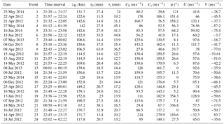
Table 1Observed and intrinsic parameters of medium-scale gravity waves over São do João do Cariri. Intrinsic parameters are denoted by “i” and observed by “o”. The propagation direction is represented by ϕ and increases clockwise from the north. The horizontal components of the wind are represented by U and V for zonal and meridional components, respectively. The “Events” column represents the sequential order used in Figs. 4 and 5.
Airglow images of two emissions, near-infrared (NIR) OH and OI6300, have routinely been taken by an all-sky imager installed in São João do Cariri since 2011. In the present work, data collected from 2012 and 2014 were used to study periodic waves in OI6300 airglow images. Simultaneous thermospheric wind data were also collected by two FPIs, one deployed at São João do Cariri and the other at Cajazeiras (6.9∘ S, 38.5∘ W).
The São João do Cariri's all-sky imager was developed by Keo Scientific. The fast (f∕0.95) imaging system uses a fisheye lens with a field of view of 180∘. The light is projected through a filter wheel with 3 inch diameter interference filters. During these observations only two filters were used, one for the OI6300 emission and another for the NIR OH emission, which is a notched wide-band filter. The images are projected onto a CCD of 1024×1024 pixels and each pixel has 13 µm of width. The sensor has a high quantum efficiency, better than 95 %, and is cooled down to −70 ∘C to reduce the dark current. Other technical details about this imager have been published elsewhere (e.g., Takahashi et al., 2015). Images of the OI6300 airglow emission have been taken using an exposure time of 90 s. Thus, high-frequency periodic waves with periods greater than 5 min can be detected by this system. The methodology to determine the spectral parameters of the periodic waves in the OI6300 emission data was published by Paulino et al. (2016).
The RENOIR project was designed to study the dynamics of the equatorial thermosphere. An important contribution of this project was measurements of the thermospheric neutral wind in the equatorial zone over the South American continent (Makela et al., 2009; Fisher et al., 2015). The FPIs used in this experiment have an interference filter of 50 mm diameter combined with an etalon of 42 mm diameter. The reflectivity of the etalon was adjusted to be 77 % in order to enhance the transmission of the light at 630 nm without effective loss of the spectral resolution. A set of lenses produces 11 rings of the interference pattern onto a CCD camera. The CCD has a resolution of 1024×1024 pixels and each pixel has 13 µm of width. A dual-mirror sky scanner controlled by two smart motors was used to observe different directions in the sky. The sky scanning was calibrated using the Sun's position with an accuracy of 0.2 per degree. An exposure time of 300 s was used to observe the OI6300 and 30 s of exposure to make frequency-stabilized laser calibration images. Further details about the design of the FPI can be found in Meriwether et al. (2011). Since the FPIs were separated by less than 250 km, measurements of thermospheric wind from either the São João do Cariri's FPI or the Cajazeiras FPI were used to estimate the components of the horizontal wind to be used in the calculation of the intrinsic frequencies of the periodic waves. As the observed waves occupied a large portion of the airglow images, this assumption is quite reasonable.
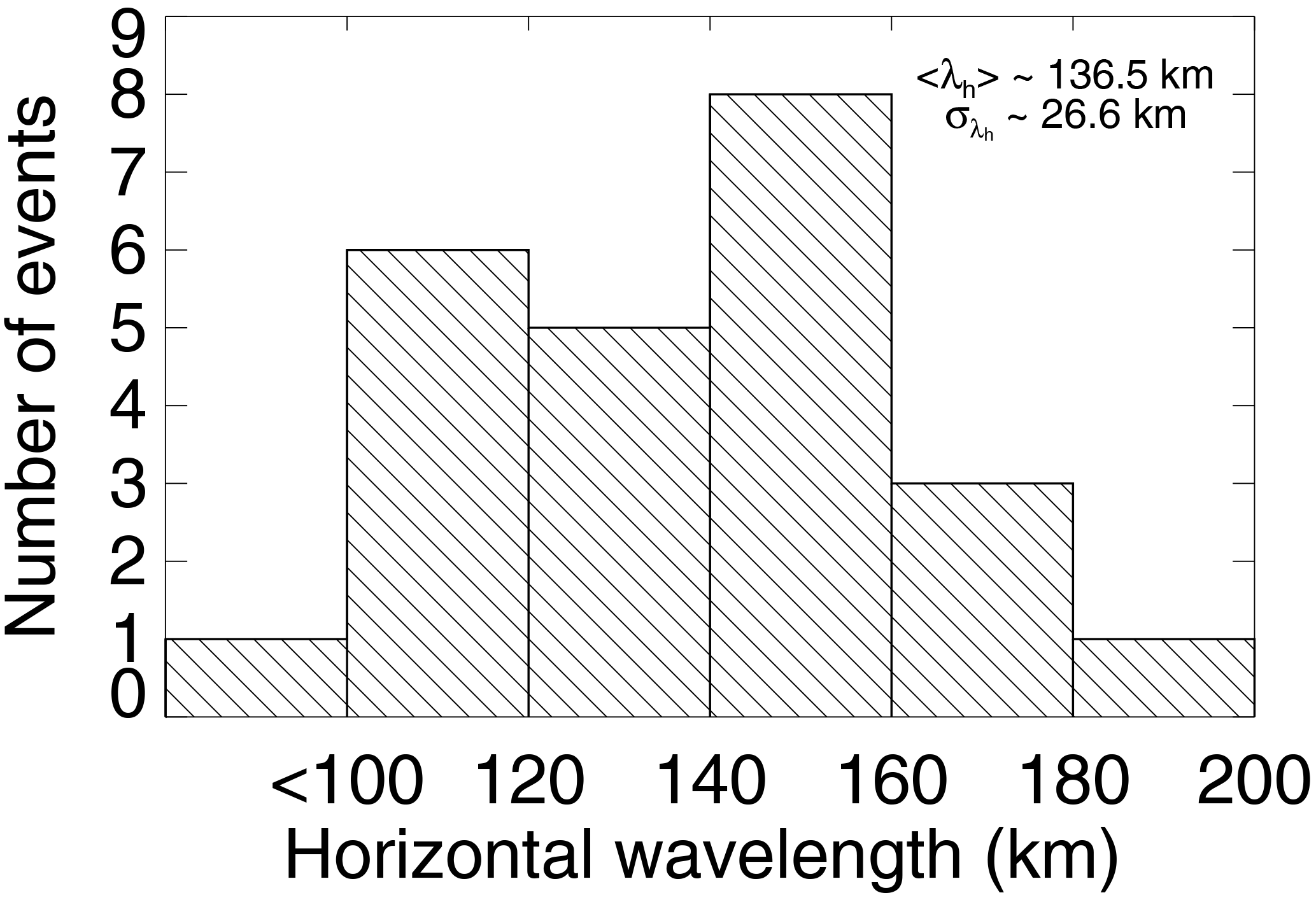
Figure 1Histogram for the wavelengths of the periodic waves. represents the average and represents the standard deviation of the mean.

Figure 2Histograms for the (a) observed periods, (b) intrinsic periods, (c) observed phase speeds and (d) intrinsic phase speeds. The number in the brackets represents the average and the standard deviation of the mean is represented by σ.
To calculate the intrinsic frequency of the periodic waves, the following equation was used:
where ωo is the observed frequency, kH is the horizontal wave vector and U is the horizontal wind interpolated to the time in which the waves were observed. Winds measured at São João do Cariri were preferred to be used. However, in some cases, the winds measured at Cajazeiras were used as well when São João do Cariri's winds were not available. From the intrinsic frequency, the intrinsic period and intrinsic horizontal phase speed can be directly estimated.
Table 1 shows all parameters of the studied periodic waves. Notice that the intrinsic parameters are denoted by the index “i”, the observed parameters are represented by the index “o”. The propagation direction is represented by ϕ and increases clockwise from the north. The horizontal components of the wind were represented by U and V for zonal and meridional components, respectively. The “Events” column represents the sequential order used in Figs. 4 and 5.
3.1 Spectral parameters
From 2012 to 2014, 24 periodic waves were observed in the airglow images with simultaneous measurement of the horizontal wind by the FPIs. Figure 1 shows the histogram for the wavelengths of the periodic waves, which ranged mostly from 100 to 180 km with an average of ∼136 km and standard deviation of ∼27 km. These results compare favorably with the results of Paulino et al. (2016) for long-term observations at the same site. Thus, the wavelength pattern of the periodic waves used in this study is representative of the typical waves observed at this site. However, comparison with other observations in low latitudes reveals, in general, that the periodic waves observed over São João do Cariri are shorter than other locations (e.g., Garcia et al., 2000; Fukushima et al., 2012; Narayanan et al., 2014).
Figure 2 shows the observed (a, c) and intrinsic (b, d) periods (a, b) and phase speeds (c, d) for the periodic waves. Most of them had periods shorter than 40 min with an average of ∼23 min and standard deviation of ∼11 min. Regarding the phase speed, there were more events between 75 and 175 m s−1 with the average around 113 m s−1 and a standard deviation of ∼43 m s−1. These results are quite similar to the previous observations at the same site (Paulino et al., 2016). In order to investigate the sources of these gravity waves, one can observe that these periodic waves have faster phase speed as compared to gravity waves observed in the MLT region at the same location (Medeiros et al., 2003; Taylor et al., 2009; Campos et al., 2016). However, simulations of the propagation of gravity waves in low latitudes via ray-tracing showed that medium-scale gravity waves could attain at maximum 200 km of altitude into the thermosphere–ionosphere (Vadas et al., 2009; Paulino et al., 2011, 2012). In this case, the sources of these two sets of waves must be different. Since the faster gravity waves are less susceptible to the wind filtering process in the atmosphere (Vadas, 2007; Vadas and Liu, 2009; Fritts and Vadas, 2008), the periodic waves must have their origin in the thermosphere and propagate upward.
Figure 2 also shows the distribution of the intrinsic parameters. Most of the waves had intrinsic periods shorter than 20 min, the average was ∼22 min (almost the same for the observed case) and the standard deviation was ∼15 min. According to the histogram for the phase speed, one can see that most waves had intrinsic phase speeds between 125 and 175 m s−1. The average of the intrinsic phase speed was ∼130 m s−1 and the standard deviation was ∼60 m s−1.
One advantage of knowing the intrinsic parameters is that the propagation characteristics (time and distance prior to dissipation, for instance) of the gravity waves can be assessed more precisely (Vadas, 2007). In this study, if most of the waves were launched from the lower thermosphere (∼120 km height), they could propagate up to the bottom of the ionospheric F region (∼250 km height) and then be observed by the OI6300 airglow images. Another important characteristic of these waves is the inclination of their propagation in the atmosphere. Since they have horizontal wavelengths of ∼140 km, on average, and the vertical wavelength must be at least ∼80 km due to the thickness of the OI6300 layer (Sobral et al., 1993), these waves must have an inclination much larger than those waves observed in the MLT, thus they can propagate quickly in the vertical (Vadas, 2007).
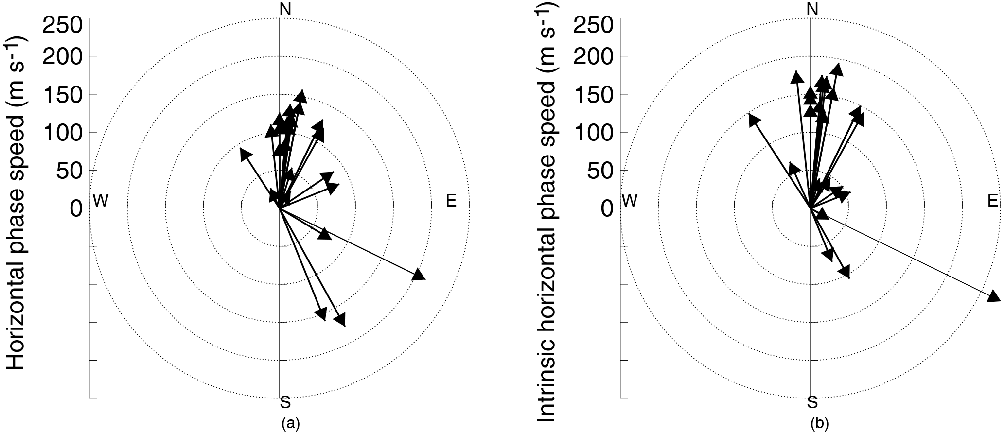
Figure 3Vector diagrams for (a) observed and (b) intrinsic phase velocities. Each circle represents an isoline of 50 m s−1.
3.2 Propagation direction
Figure 3 shows the propagation direction of the periodic waves. The chart on the left is for the observed phase velocity and the chart on the right is for the intrinsic phase velocity. Most of the waves propagated to the northeast, north and northwest and four of them propagated to the southeast, which is the same anisotropy presented by Paulino et al. (2016). Comparing the intrinsic phase velocity with the observed one, it is possible to see that the wind is decelerating most of the waves which propagate to the north. Regarding the waves propagating southeastward, three of them were decelerated.
The explanation of the increase and decrease in the observed period due to the wind can be interpreted from Eq. (1). When the periodic waves are propagating in the same direction as the wind, the second term of the right-hand side is maximized, the observed frequencies increase and the observed periods are reduced compared to the intrinsic periods. Otherwise, if the wave propagates anti-parallel to the wind direction, the observed frequencies are reduced, resulting in an increase in the observed periods.
Figure 4 shows this effect on the periodic waves observed in this study. The horizontal dashed line represents 90∘ between the wave and wind vector. For all periodic waves observed below this line, the intrinsic periods are longer than the observed periods. When the wind is close to 90∘, there is not much difference and for angles greater than 90∘, the observed periods are longer than the intrinsic periods. For event 9, the discrepancy was the largest and it happens due to the strength of the observed wind during the occurrence of this wave.
On one hand, gravity waves propagating parallel to the background wind can reach critical levels and be absorbed by the medium. On the other hand, if the propagation is anti-parallel to the wind, the gravity waves can be reflected due to turning levels. These are the reasons why fast gravity waves propagate easily into the atmosphere (Vadas and Liu, 2009). The measurements of the horizontal wind are really useful to discuss the propagation of the periodic waves. Further, in the lower part of the thermosphere which corresponds to the range of the OI6300 airglow layer according to the horizontal wind model (HWM-14; ∼ 200–300 km), the wind does not change quickly in time and altitude (Drob et al., 2015).
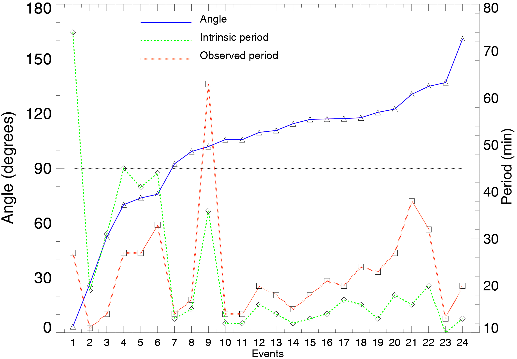
Figure 4Diagram for the angle between the propagation of periodic wave and wind vector for all 24 waves. The observed and intrinsic periods are shown on the right vertical axis.
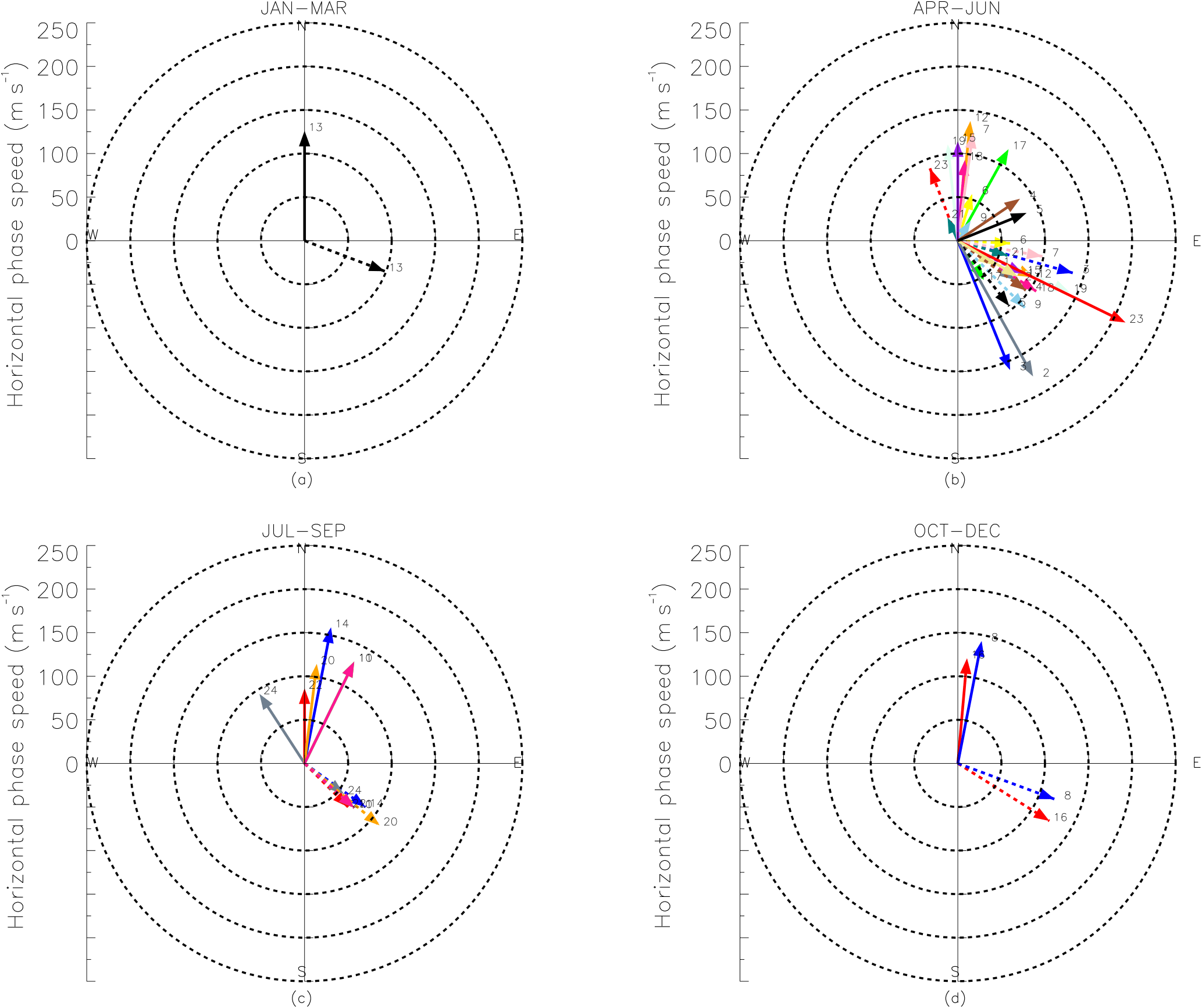
Figure 5Vector diagrams for the winds (dashed arrows) and phase velocity (solid arrows) observed during the summer (a), autumn (b), winter (c) and spring (d).

Figure 6Blocking diagrams due to the wind for the summer (a), autumn (b), winter (c) and spring (d). Theoretically, propagation of periodic waves were prohibited in the shaded areas due to the action of critical levels.
One topic that was poorly discussed in Paulino et al. (2016) is the anisotropy of the propagation direction of the periodic waves. This kind of anisotropy can have two origins: either associated with the anisotropy of the sources themselves or the filtering process of the gravity due to the wind system. Figure 5 shows a vector diagram for the phase velocity of the periodic waves (solid arrows) and horizontal wind vector (dashed arrows). The numbers in front of the arrows indicate the event numbers shown in Table 1 and Fig. 4.
The first important result from this analysis is that the wind direction derived from the FPI (∼250 km) during the evening over São João do Cariri is typically southeastward and it corresponds to the time interval of maximum occurrence of the periodic waves. As a consequence of this wind pattern, most of the observed periodic waves were propagating almost orthogonal to the wind and it is certainly the most important reason why many observed periodic waves had a propagation direction to the north at the observation site.
Furthermore, according to the Thermosphere–Ionosphere–Electrodynamics General Circulation Model (TIE-GCM; Roble and Ridley, 1994), the horizontal wind in the lower thermosphere (below 180 km height) during the evening is southwestward. Thus, periodic waves generated in the lower levels of the thermosphere are not allowed to propagate almost parallel to the southwest–northeast direction and, in the levels near the OI6300 layer, the blocking area is moved to be almost parallel to the southeast–northwest direction. As a result, only faster periodic waves are able to skip the filtering effects and can be observed in this direction. The results of Paulino et al. (2016) sustain this hypotheses indicating that the wind filtering is the main reason for the observed anisotropy in the propagation direction of periodic waves, even if the sources of them are isotropic.
Even so, few events were observed in the direction parallel or anti-parallel to the wind. In all cases, the phase speeds of the periodic waves were greater than the magnitude of the wind and it agrees with the theory. Figure 6 shows the blocking diagrams for the seasons calculated using the HWM-14 model for the heights below the OI6300 layer and from 18:00 to 24:00 LT. This time interval coincides with the time of maximum occurrence of periodic waves as mentioned above. According to the theory of the filtering process of the waves due to the wind system, propagation of periodic waves into the shaded area is not allowed; since in these cases, the waves would attain critical levels. Further details on the calculations of the blocking diagrams were published by Medeiros et al. (2003) and Campos et al. (2016). It is important to observe that none of the studied periodic wave were into the prohibited areas, i.e., indicating that all periodic waves have enough phase speed to skip the critical levels.
Furthermore, during the summer, autumn and winter, the main blocking areas are almost orthogonal to the propagation direction of the periodic waves, which help to explain the observed results. During the spring, the blocking diagram had a large area almost parallel to the propagation of the waves; however, the waves had phase velocity greater than the prohibited area, and were able to overcome the absorption level.
Thus, the usage of the blocking diagram reinforced with the FPI measurements of the wind in the same altitude of the periodic wave satisfactorily explain the propagation direction of the periodic waves over São João do Cariri.
Intrinsic parameters and effects of the wind in the propagation direction of periodic waves were studied in detail using simultaneous measurements of OI6300 airglow images and thermospheric wind by FPIs from 2012 to 2014 over São João do Cariri and the results are listed as follows:
-
The observed parameters of the waves and their anisotropy in the propagation direction were quite similar to the previous observations, indicating that the present results are representative of the typical waves observed at this site;
-
In general, the wind reduces the phase speed of the periodic waves. It suggests that these waves can have better conditions for propagating into the thermosphere by skipping critical and turning levels;
-
The main contribution of this paper is the analysis of the strength and direction of the wind in the OI6300 layer and below from the TIE-GCM model, and that the observed anisotropy can fully be explained by the filtering process of the wind even if the sources of the periodic waves are isotropic.
All-sky airglow images used in this work can be accessed on the Internet at the Brazilian Program of Space Weather (EMBRACE) webpage at (http://www2.inpe.br/climaespacial/portal/en/) and FPI data are available online at the CEDAR Archival Madrigal Database (http://cedar.openmadrigal.org).
IP supervised the data analysis and wrote most of the manuscript with the help of ARP. JFM did part of the analysis and produced all figures. GLM calculated the parameters of the periodic waves and the components of the wind. CMW wrote most of the analysis programs and helped with the language corrections. RAB, AFM and HT coordinated the experiment with the imager, operated the equipment and contributed to the text of the manuscript. JJM and JWM installed the FPIs and reduced the data contributing to the analysis by calculating the winds. JAVC calculated the blocking diagrams of Fig. 6.
The authors declare that they do not have competing interests.
This article is part of the special issue “Space weather connections to near-Earth space and the atmosphere”. It is a result of the 6∘ Simpósio Brasileiro de Geofísica Espacial e Aeronomia (SBGEA), Jataí, Brazil, 26–30 September 2016.
The present work has been supported by Conselho Nacional de
Desenvolvimento Científico e Tecnológico (CNPq) under contracts
451836/2017-0, 473473/2013-5, 301078/2013-0, 303511/2017-6 and 460624/2014-8.
The topical editor, Jean-Pierre Raulin, thanks two
anonymous referees for help in evaluating this paper.
Amorim, D. C. M., Pimenta, A. A., Bittencourt, J. A., and Fagundes, P. R.: Long-term study of medium-scale traveling ionospheric disturbances using OI 630 nm all-sky imaging and ionosonde over Brazilian low latitudes, J. Geophys. Res.-Space, 116, A06312, https://doi.org/10.1029/2010JA016090, 2011. a, b
Campos, J. A. V., Paulino, I., Wrasse, C. M., de Medeiros, A. F., Paulino, A. R., and Buriti, R. A.: Observations of small-scale gravity waves in the equatorial upper mesosphere, Revista Brasileira de Geofísica, 34, 10 pp., https://doi.org/10.22564/rbgf.v34i4.876, 2016. a, b
Candido, C. M. N., Pimenta, A. A., Bittencourt, J. A., and Becker-Guedes, F.: Statistical analysis of the occurrence of medium-scale traveling ionospheric disturbances over Brazilian low latitudes using OI 630.0 nm emission all-sky images, Geophys. Res. Lett., 35, L17105, https://doi.org/10.1029/2008GL035043, 2008. a
Drob, D. P., Emmert, J. T., Meriwether, J. W., Makela, J. J., Doornbos, E., Conde, M., Hernandez, G., Noto, J., Zawdie, K. A., McDonald, S. E., Huba, J. D., and Klenzing, J. H.: An update to the Horizontal Wind Model (HWM): the quiet time thermosphere, Earth and Space Science, 2, 301–319, https://doi.org/10.1002/2014EA000089, 2015. a
Fagundes, P. R., Sahai, Y., Batista, I. S., Abdu, M. A., Bittencourt, J. A., and Takahashi, H.: Observations of day-to-day variability in precursor signatures to equatorial F-region plasma depletions, Ann. Geophys., 17, 1053–1063, https://doi.org/10.1007/s00585-999-1053-x, 1999. a, b
Fisher, D. J., Makela, J. J., Meriwether, J. W., Buriti, R. A., Benkhaldoun, Z., Kaab, M., and Lagheryeb, A.: Climatologies of nighttime thermospheric winds and temperatures from Fabry–Perot interferometer measurements: from solar minimum to solar maximum, J. Geophys. Res.-Space, 120, 6679–6693, https://doi.org/10.1002/2015JA021170, 2015. a
Fritts, D. C. and Alexander, M. J.: Gravity wave dynamics and effects in the middle atmosphere, Rev. Geophys., 41, 1003, https://doi.org/10.1029/2001RG000106, 2003. a, b
Fritts, D. C. and Vadas, S. L.: Gravity wave penetration into the thermosphere: sensitivity to solar cycle variations and mean winds, Ann. Geophys., 26, 3841–3861, https://doi.org/10.5194/angeo-26-3841-2008, 2008. a, b, c
Fukushima, D., Shiokawa, K., Otsuka, Y., and Ogawa, T.: Observation of equatorial nighttime medium-scale traveling ionospheric disturbances in 630 nm airglow images over 7 years, J. Geophys. Res.-Space, 117, A10324, https://doi.org/10.1029/2012JA017758, 2012. a, b, c, d, e
Fukushima, D., Shiokawa, K., Otsuka, Y., Nishioka, M., Kubota, M., Tsugawa, T., Nagatsuma, T., Komonjinda, S., and Yatini, C. Y.: Geomagnetically conjugate observation of plasma bubbles and thermospheric neutral winds at low latitudes, J. Geophys. Res.-Space, 120, 2222–2231, https://doi.org/10.1002/2014JA020398, 2015. a, b
Garcia, F. J., Taylor, M. J., and Kelley, M. C.: Two-dimensional spectral analysis of mesospheric airglow image data, Appl. Optics, 36, 7374–7385, https://doi.org/10.1364/AO.36.007374, 1997. a, b
Garcia, F. J., Kelley, M. C., Makela, J. J., and Huang, C.-S.: Airglow observations of mesoscale low-velocity traveling ionospheric disturbances at midlatitudes, J. Geophys. Res., 105, 18407, https://doi.org/10.1029/1999JA000305, 2000. a, b, c, d
Kubota, M., Shiokawa, K., Ejiri, M. K., Otsuka, Y., Ogawa, T., Sakanoi, T., Fukunishi, H., Yamamoto, M., Fukao, S., and Saito, A.: Traveling ionospheric disturbances observed in the OI 630 nm nightglow images over Japan by using a Multipoint Imager Network during the FRONT Campaign, Geophys. Res. Lett., 27, 4037–4040, https://doi.org/10.1029/2000GL011858, 2000. a
Liu, J. Y., Rajesh, P. K., Lee, I. T., and Chow, T. C.: Airglow observations over the equatorial ionization anomaly zone in Taiwan, Ann. Geophys., 29, 749–757, https://doi.org/10.5194/angeo-29-749-2011, 2011. a, b
Makela, J. J., Meriwether, J. W., Lima, J. P., Miller, E. S., and Armstrong, S. J.: The remote equatorial nighttime observatory of ionospheric regions project and the international heliospherical year, Earth Moon Planets, 104, 211–226, 2009. a, b
Makela, J. J., Lognonné, P., Hébert, H., Gehrels, T., Rolland, L., Allgeyer, S., Kherani, A., Occhipinti, G., Astafyeva, E., Coïsson, P., Loevenbruck, A., Clévédé, E., Kelley, M. C., and Lamouroux, J.: Imaging and modeling the ionospheric airglow response over Hawaii to the tsunami generated by the Tohoku earthquake of 11 March 2011, Geophys. Res. Lett., 38, L00G02, https://doi.org/10.1029/2011GL047860, 2011. a, b
Martinis, C., Baumgardner, J., Wroten, J., and Mendillo, M.: All-sky imaging observations of conjugate medium-scale traveling ionospheric disturbances in the American sector, J. Geophys. Res.-Space, 116, A05326, https://doi.org/10.1029/2010JA016264, 2011. a
Medeiros, A. F., Taylor, M. J., Takahashi, H., Batista, P. P., and Gobbi, D.: An investigation of gravity wave activity in the low-latitude upper mesosphere: propagation direction and wind filtering, J. Geophys. Res.-Atmos., 108, 4411, https://doi.org/10.1029/2002JD002593, 2003. a, b
Meriwether, J. W., Makela, J. J., Huang, Y., Fisher, D. J., Buriti, R. A., Medeiros, A. F., and Takahashi, H.: Climatology of the nighttime equatorial thermospheric winds and temperatures over Brazil near solar minimum, J. Geophys. Res., 116, A04322, https://doi.org/10.1029/2011JA016477, 2011. a
Narayanan, V. L., Gurubaran, S., Emperumal, K., and Patil, P. T.: A study on the night time equatorward movement of ionization anomaly using thermospheric airglow imaging technique, J. Atmos. Sol.-Terr. Phy., 103, 113–120, https://doi.org/10.1016/j.jastp.2013.03.028, 2013. a, b
Narayanan, L. V., Shiokawa, K., Otsuka, Y., and Saito, S.: Airglow observations of nighttime medium-scale traveling ionospheric disturbances from Yonaguni: statistical characteristics and low-latitude limit, J. Geophys. Res.-Space, 119, 9268–9282, https://doi.org/10.1002/2014JA020368, 2014. a, b, c, d, e
Otsuka, Y., Onoma, F., Shiokawa, K., Ogawa, T., Yamamoto, M., and Fukao, S.: Simultaneous observations of nighttime medium-scale traveling ionospheric disturbances and E region field-aligned irregularities at midlatitude, J. Geophys. Res.-Space, 112, A06317, https://doi.org/10.1029/2005JA011548, 2007. a
Paulino, I., de Medeiros, A. F., Buriti, R. A., Takahashi, H., Sobral, J. H. A., and Gobbi, D.: Plasma bubble zonal drift characteristics observed by airglow images over Brazilian tropical region, Revista Brasileira de Geofísica, 29, 239–246, https://doi.org/10.1590/S0102-261X2011000200003, 2011. a, b, c
Paulino, I., Takahashi, H., Vadas, S., Wrasse, C., Sobral, J., Medeiros, A., Buriti, R., and Gobbi, D.: Forward ray-tracing for medium-scale gravity waves observed during the {COPEX} campaign, J. Atmos. Sol.-Terr. Phy., 90–91, 117–123, https://doi.org/10.1016/j.jastp.2012.08.006, 2012. a
Paulino, I., Medeiros, A. F., Vadas, S. L., Wrasse, C. M., Takahashi, H., Buriti, R. A., Leite, D., Filgueira, S., Bageston, J. V., Sobral, J. H. A., and Gobbi, D.: Periodic waves in the lower thermosphere observed by OI630 nm airglow images, Ann. Geophys., 34, 293–301, https://doi.org/10.5194/angeo-34-293-2016, 2016. a, b, c, d, e, f, g, h, i
Roble, R. G. and Ridley, E. C.: A thermosphere-ionosphere-mesosphere-electrodynamics general circulation model (time-GCM): equinox solar cycle minimum simulations (30–500 km), Geophys. Res. Lett., 21, 417–420, https://doi.org/10.1029/93GL03391, 1994. a
Shiokawa, K., Otsuka, Y., Tsugawa, T., Ogawa, T., Saito, A., Ohshima, K., Kubota, M., Maruyama, T., Nakamura, T., Yamamoto, M., and Wilkinson, P.: Geomagnetic conjugate observation of nighttime medium-scale and large-scale traveling ionospheric disturbances: FRONT3 campaign, J. Geophys. Res.-Space, 110, A05303, https://doi.org/10.1029/2004JA010845, 2005. a
Shiokawa, K., Otsuka, Y., and Ogawa, T.: Quasiperiodic southward moving waves in 630 nm airglow images in the equatorial thermosphere, J. Geophys. Res.-Space, 111, A06301, https://doi.org/10.1029/2005JA011406, 2006. a, b, c
Shiokawa, K., Otsuka, Y., Lynn, K. J., Wilkinson, P., and Tsugawa, T.: Airglow-imaging observation of plasma bubble disappearance at geomagnetically conjugate points, Earth Planets Space, 67, 43, https://doi.org/10.1186/s40623-015-0202-6, 2015. a, b
Sobral, J. H. A., Takahashi, H., Abdu, M. A., Muralikrishna, P., Sahai, Y., Zamlutti, C. J., de Paula, E. R., and Batista, P. P.: Determination of the quenching rate of the O(1D) by O(3P) from rocket-borne optical (630 nm) and electron density data, J. Geophys. Res., 98, 7791–7798, https://doi.org/10.1029/92JA01839, 1993. a
Takahashi, H., Wrasse, C., Otsuka, Y., Ivo, A., Gomes, V., Paulino, I., Medeiros, A., Denardini, C., Sant'Anna, N., and Shiokawa, K.: Plasma bubble monitoring by TEC map and 630 nm airglow image, J. Atmos. Sol.-Terr. Phy., 130, 151–158, https://doi.org/10.1016/j.jastp.2015.06.003, 2015. a
Taori, A., Makela, J. J., and Taylor, M.: Mesospheric wave signatures and equatorial plasma bubbles: a case study, J. Geophys. Res.-Space, 115, a06302, https://doi.org/10.1029/2009JA015088, 2010. a, b
Taylor, M. J., Bishop, M. B., and Taylor, V.: All-sky measurements of short period waves imaged in the OI(557.7 nm), Na(589.2 nm) and near infrared OH and O2 (0,1) nightglow emissions during the ALOHA-93 Campaign, Geophys. Res. Lett., 22, 2833–2836, https://doi.org/10.1029/95GL02946, 1995. a, b
Taylor, M. J., Jahn, J.-M., Fukao, S., and Saito, A.: Possible evidence of gravity wave coupling into the mid-latitude F region ionosphere during the SEEK Campaign, Geophys. Res. Lett., 25, 1801–1804, https://doi.org/10.1029/97GL03448, 1998. a
Taylor, M. J., Pautet, P.-D., Medeiros, A. F., Buriti, R., Fechine, J., Fritts, D. C., Vadas, S. L., Takahashi, H., and São Sabbas, F. T.: Characteristics of mesospheric gravity waves near the magnetic equator, Brazil, during the SpreadFEx campaign, Ann. Geophys., 27, 461–472, https://doi.org/10.5194/angeo-27-461-2009, 2009. a, b, c
Vadas, S. L.: Horizontal and vertical propagation and dissipation of gravity waves in the thermosphere from lower atmospheric and thermospheric sources, J. Geophys. Res.-Space, 112, A06305, https://doi.org/10.1029/2006JA011845, 2007. a, b, c
Vadas, S. L. and Fritts, D. C.: Thermospheric responses to gravity waves: influences of increasing viscosity and thermal diffusivity, J. Geophys. Res.-Atmos., 110, D15103, https://doi.org/10.1029/2004JD005574, 2005. a
Vadas, S. L. and Liu, H.-L.: Generation of large-scale gravity waves and neutral winds in the thermosphere from the dissipation of convectively generated gravity waves, J. Geophys. Res.-Space, 114, A10310, https://doi.org/10.1029/2009JA014108, 2009. a, b, c
Vadas, S. L., Taylor, M. J., Pautet, P.-D., Stamus, P. A., Fritts, D. C., Liu, H.-L., São Sabbas, F. T., Rampinelli, V. T., Batista, P., and Takahashi, H.: Convection: the likely source of the medium-scale gravity waves observed in the OH airglow layer near Brasilia, Brazil, during the SpreadFEx campaign, Ann. Geophys., 27, 231–259, https://doi.org/10.5194/angeo-27-231-2009, 2009. a