the Creative Commons Attribution 4.0 License.
the Creative Commons Attribution 4.0 License.
 | 10 Jan 2018
Simulating the dependence of seismo-ionospheric coupling on the magnetic field inclination
Lalit Mohan Joshi
Samireddipelle Sripathi
Muppidi Ravi Kumar
Esfhan Alam Kherani
Infrasound generated during a seismic event upon reaching the ionospheric heights possesses the ability to perturb the ionosphere. Detailed modelling investigation considering 1-D dissipative linear dynamics, however, indicates that the magnitude of ionospheric perturbation strongly depends on the magnetic field inclination. Physics-based SAMI2 model codes have been utilized to simulate the ionosphere perturbations that are generated due to the action of the vertical wind perturbations associated with the seismic infrasound. The propagation of the seismic energy and the vertical wind perturbations associated with the infrasound in the model has been considered to be symmetric about the epicentre in the north–south directions. Ionospheric response to the infrasound wind, however, has been highly asymmetric in the model simulation in the north–south directions. This strong asymmetry is related to the variation in the inclination of the Earth's magnetic field north and south of the epicentre. Ionospheric monitoring generally provides an efficient tool to infer the crustal propagation of the seismic energy. However, the results presented in this paper indicate that the mapping between the crustal process and the ionospheric response is not a linear one. These results also imply that the lithospheric behaviour during a seismic event over a wide zone in low latitudes can be estimated through ionospheric imaging only after factoring in the magnetic field geometry.
Keywords. Atmospheric composition and structure (pressure, density, and temperature) – history of geophysics (atmospheric sciences) – ionosphere (ionosphere–atmosphere interactions)
Please read the corrigendum first before continuing.
-
Notice on corrigendum
The requested paper has a corresponding corrigendum published. Please read the corrigendum first before downloading the article.
-
Article
(2959 KB)
-
The requested paper has a corresponding corrigendum published. Please read the corrigendum first before downloading the article.
- Article
(2959 KB) - Full-text XML
- Corrigendum
- BibTeX
- EndNote


The ionospheric coupling to the vibrations generated on the surface of the Earth due to the earthquakes has been known for several decades (Bolt, 1964; Davies and Baker, 1965). In the last 25 years or so, the ionosphere behaviour has been explored in order to reveal the signature of the seismic Rayleigh wave propagation (e.g. Rolland et al., 2011; Astafyeva et al., 2011). The energy transferred to the atmosphere by the lithosphere travels upwards in the form of acoustic gravity wave or simply the infrasound. The wind field associated with the seismic infrasound at ionospheric altitude transports the ionospheric plasma parallel to the magnetic field and creates perturbations whose features correlate well with that of the infrasound. Recently, Chum et al. (2012) found that the features of seismic wave packets observed on the ground using the seismometer matched exactly with the features of the ionospheric response observed using Doppler sounding. The periodicities of the ionospheric perturbations were found to be exactly similar to the Rayleigh wave periodicities. They also reported the time delay between the two to be equal to the time that the infrasound takes to travel from ground to the ionospheric heights. Astafyeva et al. (2011) reported the initial total electron content (TEC) perturbation to happen over the area of maximum crustal displacement, thus verifying the possible application of the ionospheric monitoring to understand the crustal processes. There have been many reports that have indicated the seismic perturbations to have propagated to the F region peak altitude (e.g. Artru et al., 2004; Astafyeva et al., 2011). On the other hand, many investigations have reported the ionospheric perturbations to remain confined to the bottom of the F layer (e.g. Chum et al., 2012; Maruyama et al., 2016). Likewise, different researchers have proposed different modes of acoustic propagation. Studies have found the shock acoustic wave to travel at supersonic speed up to the peak of the F layer based on the total electron content (TEC) observations. However, little can be inferred about the propagation speed of seismic perturbations in the atmosphere/ionosphere based on TEC alone, as TEC perturbation represents the integrated perturbation whose exact altitude cannot be defined. Also, the height to which the seismic infrasound will propagate is likely to depend on the intensity of the seismic event.
The high-density TEC network over Japan, in recent times, has contributed significantly to further our understanding of the lithosphere–ionosphere coupling. Apart from the seismic Rayleigh waves, tsunami waves have also been observed to perturb the atmosphere–ionosphere system. The effects of the extremely strong M9.0 earthquake that occurred in Japan on 11 March 2011 have been comprehensively studied. Liu et al. (2011) found a delay of about 450 s between the M9.0 earthquake and its effect observed in the ionosphere. They reported multiple TEC wavefronts with different horizontal propagation speeds. Tsunami waves have also been found to generate pure internal gravity waves in the atmosphere, whose effects in the ionosphere are observed after a significant time delay min (Occhipinti et al., 2008).
While the features of the atmospheric waves generated due to the seismic events will depend on the propagation characteristics of the Rayleigh waves, the ionospheric response may not be a linear one. The properties of the ionosphere are anisotropic in nature. The primary reason for this anisotropy is the orientation of the Earth's magnetic field. A qualitative assessment of anisotropy in the ionospheric response related to the inclination of the Earth's magnetic field was first proposed by Hooke (1970). The inclination of the Earth's magnetic field changes very significantly in the low latitudes in the north–south direction. Due to this, the component of the infrasound wind vector parallel to Earth's magnetic field changes. Thus the dynamical response of the ionosphere to the seismic waves is also likely to have strong anisotropy in the north–south direction. This aspect has been investigated in the present study based on a detailed model simulation. The case of the 25 April 2015 Nepal earthquake is considered for that. However, the investigation is general in nature, and can be widely applied to seismic wave propagation in low latitudes.

Figure 1Seismic observations recorded at Bhuwaneshwar (20.2∘ N, 85.8∘ E) corresponding to 25 April 2015 Gorkha earthquake (Bhuwaneshwar is located ∼800 km south of the epicentre). (a) Seismometer vertical displacement velocity (z component). A and B indicates two seismic wave packets. (b) Frequency spectrum of the vertical displacement. (c) Gaussian wave packet representation of the seismic vertical displacement velocity.
Figure 1a shows the seismometer vertical displacement velocity (Vz) recorded at Bhuwaneshwar, India, (20.2∘ N, 85.8∘ E) corresponding to the 25 April 2015 Nepal earthquake. Bhuwaneshwar is located ∼800 km south of Gorkha District (28.1∘ N, 84.8∘ E). It shows two shocks (or seismic wave packets) marked as A and B. Packet A is clearly the main shock and packet B is the aftershock that followed. The frequency spectrum of the seismic recording from Bhuwaneshwar is presented in Fig. 1b. The dominant frequency is 0.08 Hz, which corresponds to the Rayleigh wave period of 12.5 s. Mathematically this seismic event can be approximated to two Gaussian wave packets as indicated in Fig. 1c. Here the amplitudes of the reconstructed wave packets are similar to the observed amplitudes. The vertical ground motion of the seismic waves generates vertical compression waves in the atmosphere above called acoustic gravity waves (AGWs), or simply the infrasound. This infrasound gets amplified enough in the atmosphere to cause detectable perturbations in the ionospheric density. In the modelling investigation which will be presented later, the Gaussian wave packets are considered to propagate away from the epicentre on the surface of the Earth, and its amplitude is considered to reduce as , where r is the distance of a particular location from the epicentre.
It must be mentioned here that aspects of the seismo-ionospheric coupling which are being investigated are general in nature and not unique to a particular event. The case of 25 April 2015 has been considered only to define the epicentre and the Rayleigh wave propagation characteristics (Rayleigh wave period and Gaussian packets) in the model simulation. Also, in the model, the seismic energy has been hypothetically considered to propagate symmetrically in all directions, which may not be true for all seismic events (or even for the 25 April 2015 event).
The amplification of the seismic infrasound takes place as it propagates upward in the atmosphere. With increase in altitude, the atmospheric density decreases. In order to conserve the momentum associated with the vertical air particle motion, its magnitude must increase. Also, at higher altitudes, the relaxation loss comes into play. As the air particle oscillates, interchange happens between the translational and internal energy. With decrease in the density (collision frequency) at higher altitudes the efficiency of the transformation of the translational and internal energy reduces and the oscillating system tends to relax. The main relaxation losses are the classical and rotational losses (Sutherland and Bass, 2004; Bass et al., 1984). Chum et al. (2012) have also described the infrasound amplification and attenuation in details. The methodology utilized by Chum et al. (2012) has been adopted in this study to determine the infrasound amplification and attenuation in the atmosphere. The modelled amplification and attenuation of the infrasound (0.08 Hz) at different height levels with respect to the forcing on the ground is presented next.
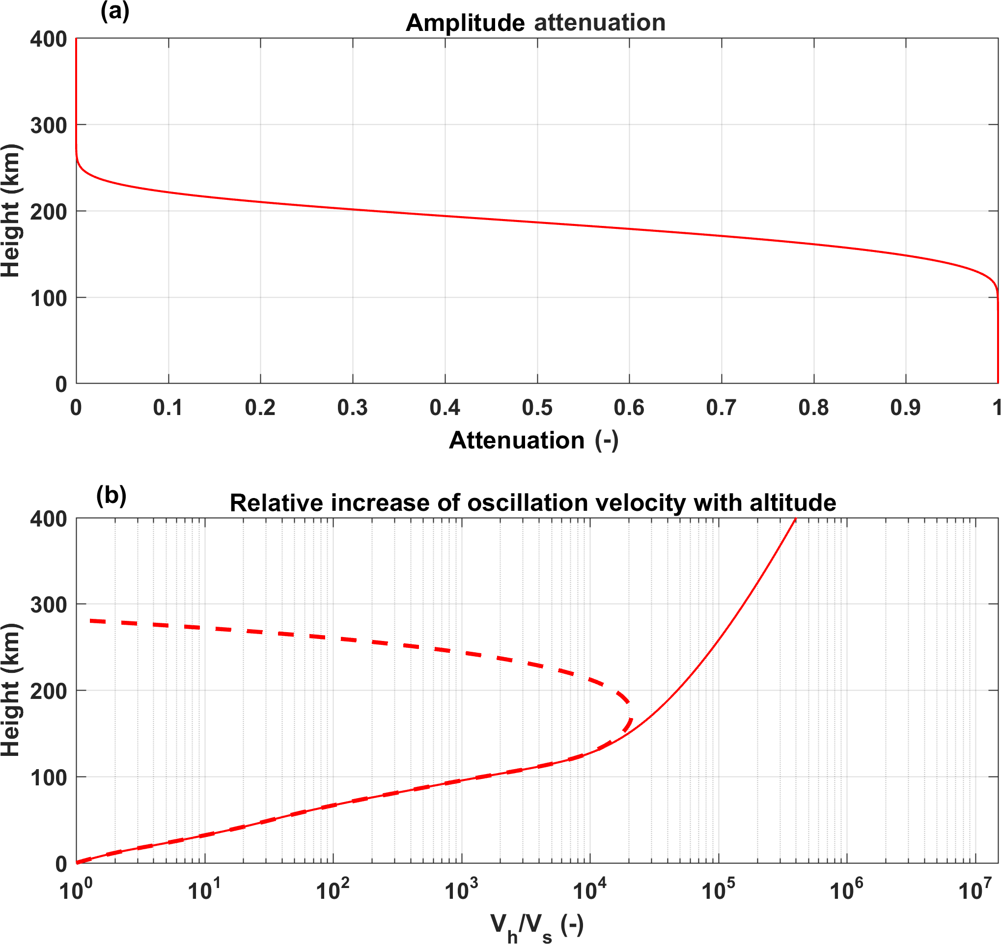
Figure 2(a) Infrasound attenuation coefficient as a function height for 12.5 s infrasound wavelength. (b) Ratio of infrasound oscillation velocity at a particular height to that on the ground (Vh∕Vs). The solid line indicates the infrasound oscillation velocity considering only the amplification. The dashed line shows the combined effect of amplification and attenuation. The methodology utilized by Chum et al. (2012) has been utilized to calculate Vh∕Vs.
Figure 2a shows the attenuation coefficient for 0.08 Hz infrasound as a function of height considering the classical and rotational relaxation loss mechanism (an excellent and detailed theoretical description of the loss mechanisms is given by Chum et al., 2012). It is interesting to see that the infrasound travels totally unattenuated up to ∼100 km altitudes. Also, the infrasound undergoes a significant amplification in the same height region to conserve the momentum associated with the oscillating air parcel. Figure 2b shows (Vh∕Vs), the ratio of infrasound amplitude at a particular height (Vh) to that at the surface of the Earth (Vs). Here, the solid line indicates Vh∕Vs considering only the amplification of the infrasound as it travel upwards. As mentioned earlier, the amplitude of the infrasound (oscillation velocity) increases with height in order to conserve the momentum of the oscillating air parcel in the atmosphere, whose density decreases exponentially with height. In reality, the attenuation of infrasound also takes place above 100 km (as discussed before) and a combined effect of amplification and attenuation decides the actual amplitude of the infrasound. The dashed line in Fig. 2b presents the ratio of infrasound amplitude at a particular height (Vh) to that at the surface of the Earth (Vs) considering the combined effect of both the amplification and the attenuation. There are two important points to note, based on the dashed line in Fig. 2a: (1) maximum amplification of ∼104 happens at ∼170 km height and (2) the infrasound is completely attenuated above 300 km height. Thus the changes in the F region ionospheric density (as a response to the seismic perturbations) can be expected mainly in its bottom side.
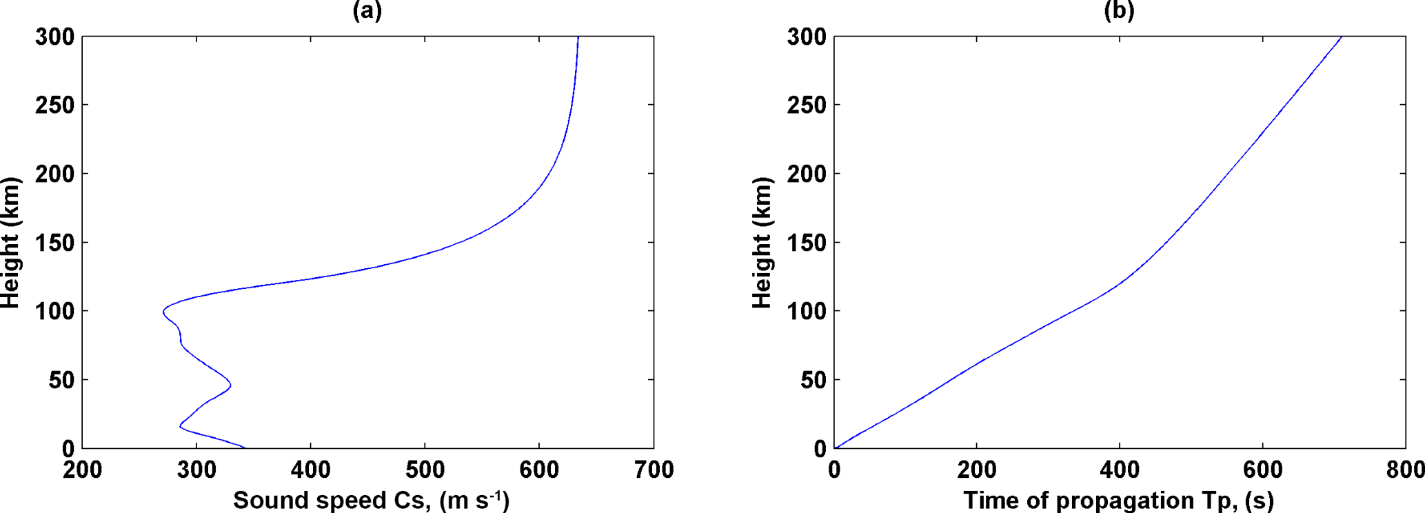
Figure 3(a) Infrasound propagation speed as a function of height. (b) Time required by infrasound to propagate from surface to various heights.
The infrasound propagation velocity and time of propagation as a function of altitude is presented in Fig. 3. Here Fig. 3a shows the infrasound speed as a function of altitude. The integrated time of propagation of the infrasound from ground to various altitudes is indicated in Fig. 3b. Here one can see that it takes s for the infrasound to propagate up to 200 km altitude (bottom F region).
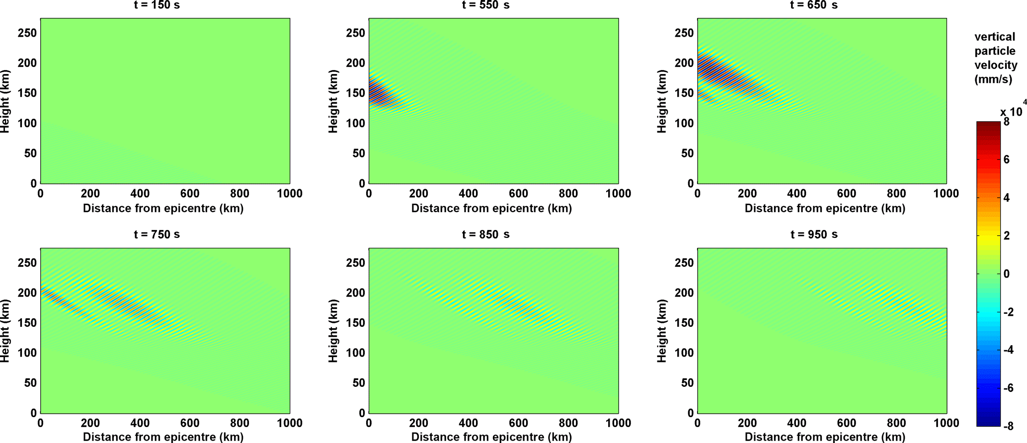
Figure 4Snapshot of the infrasound propagation in the model at six different time intervals. It took around 300–400 s for the infrasound to reach the bottom of the F layer. Two Gaussian wave packets of the infrasound can be seen. The amplitude of the infrasound vertical particle velocity can be seen decreasing as the distance from the epicentre increases, because the Rayleigh wave amplitude at the surface is considered to reduce as , where r is the distance of a particular location from the epicentre.
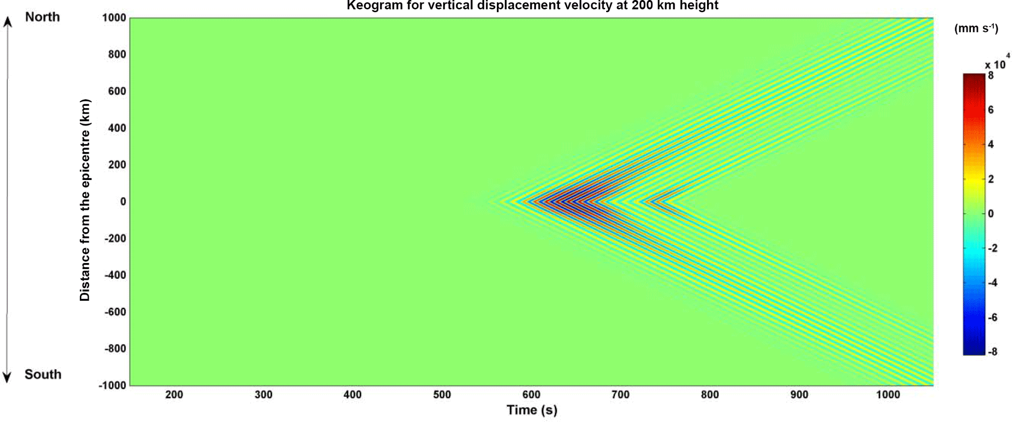
Figure 5Displacement–time diagram (keogram) of the infrasound propagation at 200 km height. The north and south arms of the keogram for the vertical particle velocity are identical, as the Rayleigh wave propagation is considered symmetric in both the north and south directions.
3.1 Vertical wind field of the infrasound in the atmosphere
The vertical displacement of the Earth's surface during a seismic event generates periodic vertical compression and rarefaction in the atmosphere. The vertical oscillation velocity of the air parcel at the surface of the Earth is of the order of a few millimetres per second (equal to the vertical velocity of the Earth's surface). However, due to the amplification at higher altitudes (as described in the previous section), the vertical wind velocity becomes quiet significant. The modelled vertical wind field associated with the seismic infrasound propagation in the atmosphere is presented in Fig. 4. Here the vertical wind field is shown for six different times after the seismic event started at the epicentre. In order to calculate the wind field over various distances from the epicentre, the Rayleigh wave amplitude at Earth's surface is assumed to reduce as (where r is the displacement on the surface of the Earth with respect to the epicentre) in such a way that its amplitude 800 km away from the epicentre is similar to the one presented in Fig. 1c. Also, the Rayleigh wave propagation on the surface of the Earth is assumed to be homogeneous in all directions for simplicity. The Rayleigh wave propagation speed is considered to be 2.4 km s−1 (Reddy and Seemala, 2015, measured the Rayleigh wave speed to be ∼2.4 km s−1 for the 25 April 2015 Nepal earthquake). From Fig. 4 one can see that it took ∼550 s for the seismic infrasound to reach the bottom-side ionospheric height over the epicentre. Likewise, the infrasound arrival at ionospheric heights away from the epicentre region happens with a further delay with respect to that over the epicentre. Note that the dynamically significant vertical wind velocity can be seen in the height region of 150 to 225 km. Above that level the amplitude reduces drastically. Chum et al. (2012) have also reported the attenuation of the infrasound due to relaxation loss process above 200 km altitude. Although the vertical displacement velocity at the surface of the Earth is just a few millimetres per second (as indicated in Fig. 1c), due to amplification the vertical wind velocity at ∼170 km altitude is of the order of mm s−1 (or 80 m s−1), which is dynamically significant enough to cause perturbations in the ionospheric densities. Also, the magnitude of the vertical wind perturbations can be seen decreasing as the distance from the epicentre increases. This is due to the reduction in the amplitude of the seismic Rayleigh wave on the surface of the Earth as it propagates away from the epicentre. Basically, the vertical wind perturbation at ionospheric height is an amplified imprint of the Rayleigh wave propagation on the Earth's surface, but with a delay of ∼300–400 s. In Fig. 4 one can also see the two Gaussian wave packet signatures in the vertical particle velocity replicating the two Gaussian wave packets (A and B) presented in Fig. 1c. These Gaussian packets in the atmosphere encapsulate the infrasound oscillations. The positive tilt of the infrasound wavefronts inside the Gaussian packets indicate that the disturbance of the vertical wind (generated due to the vertical motion of the Earth's surface) is propagating upward and away from the epicentre. The travel time diagram of the vertical wind disturbance has also been calculated to indicate the horizontal propagation of the vertical wind disturbance, which is presented in the next paragraph. In the travel time diagram, propagation in the north–south direction about the epicentre is considered.
The travel-time diagram or the keogram for the vertical particle velocity at 200 km height (ionospheric height) is presented in Fig. 5. Since the propagation of the seismic Rayleigh wave has been assumed to be uniform in all directions, the magnitude of the vertical particle velocity perturbation can be seen varying uniformly in both north and south directions. The upper half of the keogram presented in Fig. 5 is a mirror image of the bottom half. The slope of the disturbance is 2.4 km s−1 – the same as the Rayleigh wave speed considered at the surface.
The wind field presented in Fig. 4 is used as an input to the SAMI2 model to assess its impact on the ionospheric electron densities. The wind field in the north and south directions is considered to be symmetrical (as indicated by the symmetrical keogram in Fig. 5). SAMI2 is a physics-based ionospheric model which calculates the ionospheric evolution along a magnetic meridian in the north–south direction. The main objective is to simulate the differences in the ionospheric response in the north and south directions. As the magnetic field dip angle varies significantly in the north and south directions, the ionospheric response to the vertical wind perturbations associated with the infrasound can be expected to be highly non-uniform in the north and south directions. This aspect was first proposed by Hooke (1970). As a result, little attempt has been made to understand the inherent north–south asymmetry in the seismo-ionospheric coupling owing to the variation of the magnetic field inclination.

Figure 6Schematic of magnetic field parallel component of vertical wind vector at (a) magnetic equator, (b) 10∘ dip latitude, and (c) 20∘ dip latitude. The direction of magnetic field and vertical wind vector is indicated as solid and dashed black line, respectively. The red line indicates the field parallel component of vertical wind vector. As this component increases with dip latitude, the vertical wind associated with seismic infrasound will have a better efficiency to perturb the ionospheric densities at higher latitudes.
3.2 Direction of wind vector component parallel to magnetic field
Magnetic field inclination changes significantly over the low-latitude region as the location varies in the north–south direction. The inclination of the Earth's magnetic field must also play an important role in deciding the quantum of the forcing that the seismic infrasound can have on the ionosphere. A pictorial description of the wind vector component parallel to the Earth's magnetic field over the magnetic equator and low latitudes is indicated in Fig. 6, where a schematic of the vectors is shown for magnetic equator, 10∘ dip and 20∘ dip. The solid black line and dashed black line indicate the magnetic field inclination and the vertical wind vector, respectively. The component (or projection) of the vertical wind vector parallel to the magnetic field is indicated as a red line. Due to the horizontal magnetic field, there is no component of vertical wind vector parallel to the magnetic field over the magnetic equator. Over low latitudes at 10∘ dip and 20∘ dip the component of vertical wind vector can be seen as indicated by red lines. Also, the red line for the 20∘ dip is larger than that for the 10∘ dip. Thus the component of the vertical wind vector parallel to the Earth's magnetic field varies significantly with the dip latitude. This indicates that the dynamical forcing on the ionosphere due to the vertical wind associated with the infrasound is also likely to vary significantly with the dip latitude. This aspect is being simulated using the SAMI2 model to assess the inherent asymmetry in the ionospheric response in the north–south direction.

Figure 7Vertical (a) and horizontal (b) components of the particle velocity associated with the infrasound at 200 km altitude. Green and red colours indicate different epicentral distances. Note that the vertical component is significant in comparison to the horizontal.
3.3 First-order horizontal component of infrasound wind vector.
Although the seismic forcing on the atmosphere is in the vertical direction, the infrasound propagation vector may not be exactly vertical. The magnitude of the vertical forcing decreases as one moves away from the epicentre because the Rayleigh wave amplitude decreases by away from the epicentre. The pressure fluctuation front associated with the infrasound will not travel exactly vertical but will be slightly tilted (note that the wavefront in Fig. 4 is tilted; also, the x and y axes in Fig. 4 are not of the same scale, and thus this tilt is not very large). Thus, there also exists a finite horizontal wind component associated with the seismic infrasound. However, this horizontal wind component will not be directly proportional to the horizontal tilt in the infrasound propagation front (as the actual propagation of the infrasound is in the vertical direction). The tilt in the infrasound wavefront will be more in the case of the tsunami-generated infrasound than in the case of the earthquake-generated infrasound (because the tsunami waves propagate with a much lower speed in the horizontal direction, even less than the infrasound propagation speed). The first-order horizontal wind component will be equal to the horizontal difference in the vertical wind forcing. Thus, the horizontal component of the infrasound wind will be greater if the tilt in the infrasound wavefront increases. The first-order horizontal wind component has been calculated. Figure 7 shows the particle velocity associated with the infrasound at an altitude of 200 km. Here, panels (a) and (b) indicate the vertical and horizontal components of the particle velocity, respectively. These components are shown for location 200 km from epicentre (red) and 400 km from epicentre (green). The horizontal component is significantly smaller than the vertical component. This is expected as the forcing is primarily in the vertical direction. The perturbations in the ionosphere will be mainly controlled by the vertical component. There will be a contribution in the ionospheric perturbations due to the horizontal component of the infrasound wind. However, it will be much smaller than that due to the vertical component. For the ionospheric simulation in this paper only the vertical wind effects have been considered.
Some of the factors that determine the ionospheric density (electron density) are solar flux, electric field, neutral winds and thermospheric neutral density. Over the short timescales like that of the infrasound, the dynamical forcing, however, dominates. The vertical neutral wind associated with the infrasound in the bottom of the F region will have a component parallel to the magnetic field line. This field parallel component of the vertical wind can transport the ionospheric plasma along the magnetic field line. As the vertical wind will oscillate, the ionospheric density will also oscillate. However, the field parallel component of the vertical wind will depend on the dip angle of the magnetic field (as described in the previous section). Over the magnetic equator the field parallel component will be zero, and thus the ionospheric transport associated with the seismic infrasound is also likely to be negligible. The magnetic field perpendicular component of the vertical wind associated with the seismic infrasound has never been considered important in the literature as a cause of perturbations in the ionospheric densities. This is mainly because the horizontal scale size of the Rayleigh waves which produces infrasound is not sufficiently large to cause changes in the F region dynamo. Wind flow perpendicular to the magnetic field will generate electric field; however, as the magnetic field lines are highly conducting, the generated electric field will map along the field lines. If the horizontal scale of the vertical wind perturbations associated with the seismic infrasound is much less than the extent of the magnetic field line in the ionosphere, the upward and downward component of the infrasound vertical wind which will produce electric field perturbation of opposite polarity will be partially cancelled out along the field line. While the electric field related perpendicular transport will manifest along the entire field line (as the field line is nearly equipotential), wind transport parallel to the magnetic field line can be highly localized. Thus all the earlier works on seismic infrasound effects in the ionosphere have considered only the wind forcing parallel to the magnetic field lines (Artru et al., 2004; Astafyeva and Heki, 2009; Chum et al., 2012). Recently, Huba et al. (2015) have considered the magnetic field perpendicular component of the vertical wind perturbation to generate electric field. However, in that study tsunami waves were investigated. The vertical wavelength of the tsunami-generated infrasound is much larger than that for the seismic Rayleigh waves. Thus, in the present investigation, dynamical forcing parallel to the magnetic field has only been considered (as was the case with several earlier investigations). The vertical wind perturbation shown in Fig. 4 has been considered to prevail at the ionospheric heights and its impact on the ionosphere has been ascertained using the SAMI2 model. Although the vertical wind in the model is considered symmetric in north–south directions (Figs. 4 and 5), its component parallel to the magnetic field will not be symmetric in north–south directions because the magnetic field inclination itself will vary in north–south directions about the epicentre (as described in Fig. 6). Over the magnetic equator, magnetic field inclination will be zero, while at higher latitudes magnetic field inclination will increase. Thus, in the vicinity of the magnetic equator the vertical wind will have no component parallel to the magnetic field. As a consequence, the ionospheric response to the seismic infrasound over the latitudes closer to the magnetic equator is expected to be very weak in comparison to that over higher latitudes. These aspects have been investigated using the SAMI2 model.
SAMI2 is an open-source physics-based ionospheric model. Like other physics-based models (e.g. SUPIM) SAMI2 uses a magnetic field coordinate system to define a particular location in the ionosphere (Huba et al., 2000). A particular location is defined by a magnetic field line number (nf) at the apex of the magnetic field and a magnetic field segment (nz) along a magnetic field line (Huba et al., 2000). Such a coordinate system is different from the Cartesian coordinate system. In the Cartesian system the separation between any two adjacent grid points is the same, whereas in the magnetic field coordinate system they are not. In the magnetic field coordinate system, the resolution decreases (increases) with the altitude (latitude). Such a coordinate system does not pose a problem for the simulation of the large-scale processes like equatorial ionization anomaly (EIA). However, such a coordinate system may have a problem in the simulation of the seismic infrasound effects, if the separation between two grid points becomes more than half of the infrasound wavelength, anywhere in the ionospheric region under consideration. In order to overcome this problem, the SAMI2 simulation is run with a very high resolution, such that at least one grid point is located every 2.5 km altitudinal by 2.5 km latitudinal spacing. After the simulation run, the average output electron density is calculated for every 2.5 km altitudinal by 2.5 km latitudinal spacing. The simulation has been run with a time resolution of 3 s. A time resolution of 3 s is good enough to ascertain the ionospheric response to infrasound with a time period of 12.5 s (satisfying the Nyquist criterion). The response of the ionosphere in the SAMI2 model to the seismic infrasound perturbation is presented next.
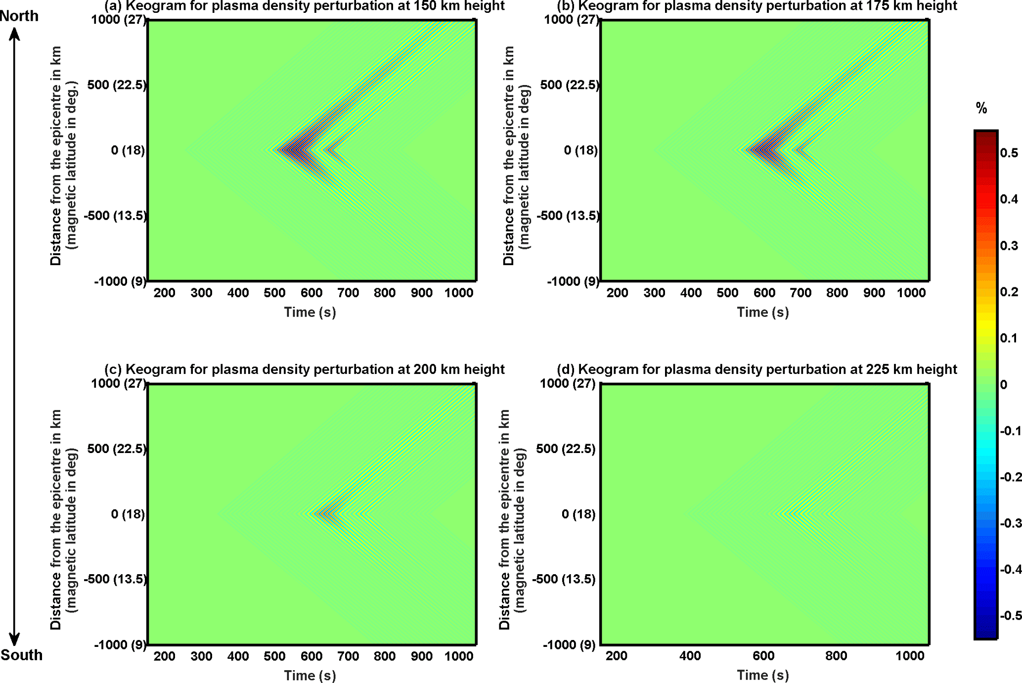
Figure 8Ionospheric response to the seismic infrasound in the SAMI2 model. (a–d) Displacement–time diagrams (keogram) of ionospheric perturbations at 150, 175, 200 and 225 km heights, respectively. Even though the infrasound propagation (as shown in Fig. 3b) is symmetric in north–south directions, the ionospheric response to it in SAMI2 model is asymmetric.
Figure 8 shows the travel-time diagram (keogram) for the ionospheric density perturbation (in %) related with the infrasound forcing in the SAMI2 simulation. In Fig. 8, the travel-time diagram has been shown for four different height levels. Panels (a), (b), (c), and (d) indicate the travel-time diagram at 150, 175, 200 and 225 km height, respectively. The x axis in these keograms indicates the distance from the epicentre with the magnetic latitude indicated in parentheses. The signatures of the two Gaussian wave packets are clearly visible in these keograms. Two of the most important aspects of the ionospheric perturbations in Fig. 8 are as follows: (1) the amplitude of the perturbation is quite small at 225 km height in comparison to that below ∼200 km altitude, and (2) the perturbation amplitude is significantly asymmetric in the north and south directions at all height levels. As far as the height variation is concerned, it is related to the reduced neutral wind perturbation amplitude at heights above 200 km (Fig. 4). Recently, Maruyama et al. (2016) have observed the deformation in the lower-frequency edge of the ionograms at the time of the arrival of the seismic infrasound in the ionosphere. They have also reported the ionospheric perturbations in the height range below 200 km. An interesting aspect, however, is the north–south asymmetry in the ionospheric density fluctuations. The geomagnetic field inclination angle northward of the Gorkha district (epicentre) will increase, while in the southward direction it will decrease (as we move towards the magnetic equator). As a consequence, the field parallel component of the vertical wind will also increase (decrease) as we travel northward (southward) of the epicentre (note that the magnetic latitude is indicated in parentheses in the x axis in Fig. 8). Thus, considering the uniform distribution of the seismic energy in all directions, the ionospheric impact of the seismic infrasound is highly non-uniform in north and south directions.
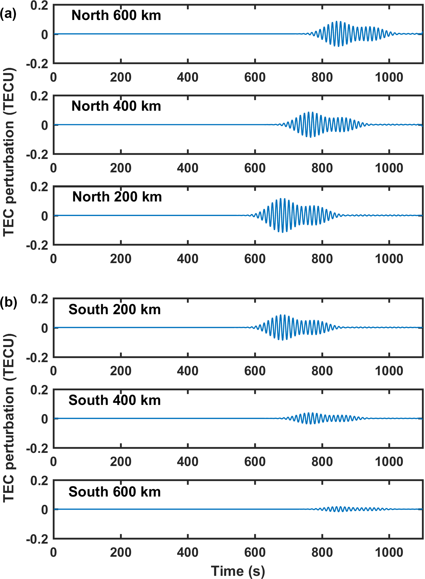
Figure 9TEC perturbations in the SAMI2 model over six different locations along north–south direction about the epicentre: (a) shows TEC perturbation amplitude in the north direction, while (b) shows it for the south direction. Note that the TEC perturbation amplitude reduces drastically in the south direction.
Most of the investigations on the propagation of the seismic infrasound in the ionosphere have utilized the TEC measurements. TEC provides the integrated ionospheric perturbation along the line of sight from ground to the GPS satellite. Detectable TEC perturbation can be expected along a line of sight, where successive ionospheric density fluctuations add up in phase (Artru et al., 2005). Such a scenario happens for line-of-sight elevation angles less than 40∘. In the model, the perturbations in the TEC in response to the seismic infrasound have also been calculated. Figure 9 presents the TEC perturbations in the SAMI2 model over six different locations in the north–south direction about the epicentre. In Fig. 9, top (bottom) three panels shows the TEC perturbations in the SAMI2 model over locations 200, 400 and 600 km away from the epicentre in the north (south) directions. Two of the important aspects of the TEC perturbations are that (a) the perturbation amplitude reduces much faster in the south direction than in the north direction, and (b) the signature of two Gaussian packets are not as distinct in the TEC as in the density perturbations at a particular altitude (as seen in the keograms in Fig. 8). The former is related to the higher magnetic field parallel component of the vertical wind perturbations in the north direction (owing to a higher inclination of the magnetic field lines). As far as the signatures of the two Gaussian seismic packets are concerned, it can be expected to be less distinct in the TEC as TEC is an integrated entity. Ionospheric density perturbations from both the Gaussian packets will be integrated along the line of sight at the junction of the two Gaussian packets in the TEC if the time interval between the two Gaussian packets is not sufficiently large.
Ionospheric monitoring and simulation with respect to seismic activities have attracted much attention due to its possible application in the remote detection of the propagation of the seismic waves. Also, the ionospheric modelling has a very prominent role to play in tsunami forecasting as the tsunami wave travels much more slowly than the Rayleigh waves and the infrasound in the atmosphere, so the lead time of forecast can be in excess of a few tens of minutes. Recently, Astafyeva et al. (2011) have succeeded in retrieving the image of the crustal slip associated with the Tohoku-oki earthquake from the TEC measurement using a high-density GPS receiver network. Modelling investigations on the other hand could reproduce the wider-scale TEC disturbances due to the 2011 Tohoku-oki tsunami (Kherani et al., 2012). Most of the investigations on the ionospheric response to seismic events using the networked observations have been made over the mid-latitudes. In the low-latitude regions, the 26 December 2004 Sumatra tsunami has been investigated comprehensively for its signature in the ionosphere (e.g. Otsuka et al., 2006; Occhipinti et al., 2008). Some of these investigations have indicated the role of the geomagnetic field inclination in deciding the ionospheric response to the internal gravity waves (IGWs) driven by the tsunami. IGWs are pure gravity waves which take more than ∼30 min to propagate to the ionospheric height. The majority of investigations have, however, reported the response time in the ionosphere to be less than 10 min, which is only possible if the atmospheric waves travel with a velocity not less than the infrasound propagation velocity. Thus the prominent carrier of the seismic energy to the ionospheric heights is the infrasound. The magnetic field parallel component of the vertical motion associated with the seismic infrasound perturbs the ionosphere along the field line (Artru et al., 2004; Chum et al., 2012). Thus, the response of the ionosphere to the seismic infrasound must also vary with the inclination of the Earth's magnetic field.
The model for AGWs in this investigation has followed 1-D dissipative linear dynamics. Most of the earlier investigations have followed a similar approach for infrasound propagation (e.g. Artru et al., 2004). Normal-mode vertical wind models associated with the AGWs have been found to be in a very good quantitative agreement with the ionospheric observations (Artru et al., 2004). Some recent works have also indicated the atmosphere to follow non-linear dissipative dynamics with multiple modes of AGW propagation (e.g. Liu et al., 2011). Such an approach is likely to be more applicable to tsunamis than the crustal motion associated with the earthquake, as tsunami forcing may persist for a longer duration to generate modes of pure gravity waves in addition to infrasounds. In the case of earthquakes, recent Doppler sounding observations by Chum et al. (2012) have clearly indicated that the vertically propagating infrasound associated with the vertical crustal motion can explain the pattern of the ionospheric response at different altitudes. Thus the model for AGW propagation considering 1-D dissipative linear dynamics can quite fairly represent the actual scenario.
In the present modelling investigation, the propagation characteristics of the seismic Rayleigh waves have been considered to be identical in the north–south directions about the epicentre. Thus the coupling of the lithosphere with the atmosphere was also identical in the north–south direction, as a consequence of which the infrasound propagation was identical in the model (Fig. 5). However, the ionospheric response in the model has been found to be highly asymmetric in the north–south directions (Figs. 8 and 9). The vertical motion of the neutrals associated with the seismic infrasound has the capability to move the ions along the field lines. However, in the latitudes closer to the magnetic equator, owing to a lesser inclination of magnetic field, vertical motion of neutrals will not have a significant component parallel to the magnetic field. Thus, an asymmetry was seen in the north–south direction about the epicentre in the model simulation. Over mid-latitudes, ionospheric response to seismic event has been effectively used to infer the crustal wave propagation and also crustal slips associated with the seismic events (Astafyeva et al., 2011). However, such crustal slip study has been performed for a narrow zone of ∼100 km, within which the magnetic field inclination can be considered to be constant. Also, over the mid-latitudes, the magnetic field inclination does not change drastically within a limited belt. However, if the crustal studies are to be performed over a wider zone in the lower latitudes based on the ionospheric mapping, the asymmetric nature of the ionospheric response in the north–south directions owing to the geo-magnetic field inclination must be taken into account.
The model simulations presented in Figs. 8 and 9 indicate a greater ionospheric response in the north direction. This should not be confused with some previous studies like Heki and Ping (2005) which have indicated the perturbations in the ionosphere to propagate with a higher velocity in the south direction. The distribution of the seismic energy in this investigation has been considered to be symmetrical in all directions. However, if in the actual scenario the seismic energy propagation itself is highly asymmetric, its signature will also be seen in the ionospheric observations. Otsuka et al. (2006) have also reported a greater response of the ionosphere to tsunami waves in the northern direction (see Fig. 1 of Otsuka et al., 2006). Their interpretation was similar to that adopted in this investigation. However, in the present investigation the main focus is to understand the asymmetric ionospheric response based on the physics-based SAMI2 model. The main purpose of the present investigation is to show that seismic propagation on the Earth's surface does not map linearly in terms of the ionospheric response. There does exist an inherent asymmetry in the ionospheric response due to the variation in the inclination of the Earth's magnetic field with location. However, the actual direction of propagation and also the amplitude of the ionospheric disturbances associated with the seismic event will depend most importantly on the actual direction of the propagation of seismic energy in the Earth's crust (which will depend on the crustal processes). Thus, Astafyeva et al. (2011) could reproduce the features of crustal slips associated with the seismic event based on ionospheric imaging. Future investigations must involve the simultaneous crustal and ionospheric observations to further understand the asymmetry in the mapping.
To capture the geomagnetic dependence in totality, the 3-D infrasonic model should be implemented. Employing 1-D and 3-D normal-mode modelling, Artru et al. (2004) showed that the surging time and amplitude of ionospheric response are similar in 1-D and 3-D approaches. This is expected since the low-latitude ionospheric change is mainly governed by the infrasonic wind component perpendicular to the magnetic field (Kherani et al., 2009). On this basis, the results in the present study of 1-D modelling are reasonable to the first order. The first-order contribution is evident during many seismic events. For example, the seismic vibrations are imaged in the ionosphere without significant alterations (Chum et al., 2012). Since the vertical displacement of earth or ocean surface is the primary forcing, the vertical displacement of the ionospheric layer is expected to produce the first-order effects, to preserve the seismic waveform image in the ionosphere.
Data used in this study can be obtained by contacting the corresponding author.
The authors declare that they have no conflict of interest.
This article is part of the special issue “Space weather connections to near-Earth space and the atmosphere”. It is a result of the 6∘ Simpósio Brasileiro de Geofísica Espacial e Aeronomia (SBGEA), Jataí, Brazil, 26–30 September 2016.
Lalit Mohan Joshi is thankful to the Indian Institute of Geomagnetism for the award of the “Nanabhoy Moos” Research
Fellowship. This work uses the SAMI2 ionosphere model written and developed by the Naval Research Laboratory. Open-source SAMI2 codes
are available at the NRL website (http://www.nrl.navy.mil/ppd/branches/6790/sami2). Muppidi Ravi Kumar would like to
acknowledge the Indian National Centre for Ocean Information Services (INCOIS) for providing the Bhuwaneshwar seismometer
data. The Bhuwaneshwar seismometer data used in this study can be accessed by readers through the corresponding author or by contacting
INCOIS.
The topical editor, Ricardo Arlen Buriti, thanks two
anonymous referees for help in evaluating this paper.
Artru, J., Farges, T., and Lognonné, P.: Acoustic waves generated from seismic surface waves: propagation properties determined from Doppler sounding observations and normal-mode modeling, Geophys. J. Int., 158, 1067–1077, https://doi.org/10.1111/j.1365-246X.2004.02377.x, 2004.
Artru, J., Ducic, V., Kanamori, H., Lognonné, P., and Murakami, M.: Ionospheric detection of gravity waves induced by tsunamis, Geophys. J. Int., 160, 840–848, https://doi.org/10.1111/j.1365-246X.2005.02552.x, 2005.
Astafyeva, E. and Heki, K.: Dependence of waveform of near-field coseismic ionospheric disturbances on focal mechanisms, Earth Planets Space, 61, 939–943, 2009.
Astafyeva, E., Lognonné, P., and Rolland, L.: First ionospheric images of the seismic fault slip on the example of the Tohoku-oki earthquake, Geophys. Res. Lett., 38, L22104, https://doi.org/10.1029/2011GL049623, 2011.
Bass, H. E., Sutherland, L. C., Piercy, J., and Evans, L.: Absorption of sound by the atmosphere, in: Physical Acoustics, vol. 17, edited by: Mason, W. P. and Thurston, R. N., Chap. 3, 145–232, Academic, New York, 1984.
Bolt, B. A.: Seismic airwaves from the great alaska earthquake, Nature, 202, 1095–1096, 1964.
Chum, J., Hruska, F., Zednik, J., and Lastovicka, J.: Ionospheric disturbances (infrasound waves) over the Czech Republic excited by the 2011 Tohoku earthquake, J. Geophys. Res.-Space, 117, A08319, https://doi.org/10.1029/2012JA017767, 2012.
Davies, K. and Baker, D.: Ionospheric effects observed around the time of the Alaskan earthquake of March 28, 1964, J. Geophys. Res., 70, 1251–1253, 1965.
Heki, K. and Ping, J.: Directivity and apparent velocity of the coseismic traveling ionospheric disturbances observed with a dense GPS network, Earth Planet. Sc. Lett., 236, 845–855, 2005.
Hooke, W. H.: The ionospheric response to internal gravity waves: 1. The F2 region response, J. Geophys. Res., 75, 5535–5544, https://doi.org/10.1029/JA075i028p05535, 1970.
Huba, J. D., Joyce, G., and Fedder, J. A.: Sami2 is Another Model of the Ionosphere (SAMI2): a new low-latitude ionosphere model, J. Geophys. Res.-Space, 105, 23035–23053, https://doi.org/10.1029/2000JA000035, 2000.
Huba, J. D., Drob, D. P., Wu, T.-W., and Makela, J. J.: Modeling the ionospheric impact of tsunami-driven gravity waves with SAMI3: Conjugate effects, Geophys. Res. Lett., 42, 5719–5726, https://doi.org/10.1002/2015GL064871, 2015.
Kherani, E. A., Lognonné, P., Kamath, N., Crespon, F., and Garcia, R.: Response of the ionosphere to the seismic trigerred acoustic waves: electron density and electromagnetic fluctuations, Geophys. J. Int., 176, 1–13, https://doi.org/10.1111/j.1365-246X.2008.03818.x, 2009.
Kherani, E. A., Lognonne, P., Hebert, H., Rolland, L., Astafyeva, E., Occhipinti, G., Coısson, P., Walwer, D., and de Paula, E. R.: Modelling of the total electronic content and magnetic field anomalies generated by the 2011 Tohoku-Oki tsunami and associated acoustic-gravity waves, Geophys. J. Int., 191, 1049–1066, https://doi.org/10.1111/j.1365-246X.2012.05617.x, 2012.
Liu, J.-Y., Chen, C.-H., Lin, C.-H., Tsai, H.-F., Chen, C.-H., and Kamogawa, M.: Ionospheric disturbances triggered by the 11 March 2011 M9.0 Tohoku earthquake, J. Geophys. Res., 116, A06319, https://doi.org/10.1029/2011JA016761, 2011.
Maruyama, T., Yusupov, K., and Akchurin, A.: Interpretation of deformed ionograms induced by vertical ground motion of seismic Rayleigh waves and infrasound in the thermosphere, Ann. Geophys., 34, 271–278, https://doi.org/10.5194/angeo-34-271-2016, 2016.
Occhipinti, G., Kherani, E. A., and Lognonn'e, P.: Geomagnetic dependence of ionospheric disturbances induced by tsunamigenic internal gravity waves, Geophys. J. Int., 173, 753–755, https://doi.org/10.1111/j.1365-246X.2008.03760.x, 2008.
Otsuka, Y. et al.: GPS detection of total electron content variations over Indonesia and Thailand following the 26 December 2004 earthquake, Earth Planets Space, 58, 159–165, 2006.
Sutherland, L. C. and Bass, H. E.: Atmospheric absorption in the atmosphere up to 160 km, J. Acoust. Soc. Am., 115, 1012–1032, https://doi.org/10.1121/1.1631937, 2004.
Reddy, C. D. and Seemala, G. K.: Two-mode ionospheric response and Rayleigh wave group velocity distribution reckoned from GPS measurement following Mw 7.8 Nepal earthquake on 25 April 2015, J. Geophys. Res.-Space, 120, 7049–7059, https://doi.org/10.1002/2015JA021502, 2015.
Rolland, L. M., Lognonné, P., and Munekane, H.: Detection and modeling of Rayleigh wave induced patterns in the ionosphere, J. Geophys. Res.-Space, 116, A05320, https://doi.org/10.1029/2010JA016060, 2011.
- Abstract
- Introduction
- Vertical displacement of the Earth surface associated with seismic Rayleigh waves
- Propagation of seismic infrasound in the atmosphere
- Ionospheric response to seismic infrasound
- Discussion and concluding remarks
- Data availability
- Competing interests
- Special issue statement
- Acknowledgements
- References
The requested paper has a corresponding corrigendum published. Please read the corrigendum first before downloading the article.
- Article
(2959 KB) - Full-text XML
- Abstract
- Introduction
- Vertical displacement of the Earth surface associated with seismic Rayleigh waves
- Propagation of seismic infrasound in the atmosphere
- Ionospheric response to seismic infrasound
- Discussion and concluding remarks
- Data availability
- Competing interests
- Special issue statement
- Acknowledgements
- References