Cross-correlation and cross-wavelet analyses of the solar wind IMF B_z and auroral electrojet index AE coupling during HILDCAAs

Solar-wind–geomagnetic activity coupling during high-intensity long-duration continuous AE (auroral electrojet) activities (HILDCAAs) is investigated in this work. The 1 min AE index and the interplanetary magnetic field (IMF) B_z component in the geocentric solar magnetospheric (GSM) coordinate system were used in this study. We have considered HILDCAA events occurring between 1995 and 2011. Cross-wavelet and cross-correlation analyses results show that the coupling between the solar wind and the magnetosphere during HILDCAAs occurs mainly in the period ≤ 8 h. These periods are similar to the periods observed in the interplanetary Alfvén waves embedded in the high-speed solar wind streams (HSSs). This result is consistent with the fact that most of the HILDCAA events under present study are related to HSSs. Furthermore, the classical correlation analysis indicates that the correlation between IMF B_z and AE may be classified as moderate (0.4–0.7) and that more than 80 % of the HILDCAAs exhibit a lag of 20–30 min between IMF B_z and AE. This result corroborates with Tsurutani et al. (1990) where the lag was found to be close to 20–25 min. These results enable us to conclude that the main mechanism for solar-wind–magnetosphere coupling during HILDCAAs is the magnetic reconnection between the fluctuating, negative component of IMF B_z and Earth's magnetopause fields at periods lower than 8 h and with a lag of about 20–30 min.

Keywords. Magnetospheric physics (solar-wind–magnetosphere interactions)

1 Introduction

The main mechanism of energy/momentum transfer from the solar wind to the Earth's magnetosphere is magnetic reconnection (Dungey, 1961; Akasofu, 1981). When the interplanetary magnetic field (IMF) lines are southwardly oriented, that is, antiparallel to the lines of the geomagnetic field, the frozen-in plasma condition is broken in a small region in the magnetopause. When this happens, the IMF and the geomagnetic field connect in this region, known as the diffusion region. Once connected, the IMF lines are drawn into the magnetosphere tail position, where they reconnect again (Dungey, 1961). This reconnection allows the penetration of the solar wind plasma flow into the inner magnetosphere (Cowley, 1995). Thus, the entry of energy from the solar wind into the inner magnetosphere is mainly controlled by the orientation of the IMF lines, mostly with their southward component. However, the enhanced energy transfer takes place mainly during the geomagnetic storms and substorms, when such condition is achieved (e.g., Gonzalez et al., 1994).

In addition to magnetic storms and substorms, another kind of geomagnetic activity, known as the high-intensity long-duration continuous AE (auroral electrojet) activity (HILDCAA), was identified by Tsurutani and Gonzalez (1987). They suggested four criteria for characterizing the HILDCAA events: (i) the peak AE index must be ≥ 1000 nT at least once during the event, (ii) the AE index should not decrease below 200 nT for longer than 2 h at a time, (iii) the event must continue for a minimum of 2 days, and (iv) the event must occur outside of the main phase of a geomagnetic storm.

The main cause of the HILDCAAs was suggested to be the magnetic reconnection between the magnetopause field and the southward IMF B_z in the Alfvén waves embedded in the high-speed solar wind streams (HSSs) (Tsurutani and Gonzalez, 1987; Tsurutani et al., 1990b). The HSSs are emanated from the coronal holes located in the polar regions of the Sun (Sheeley et al., 1976) and are embedded with Alfvénic fluctuations (Belcher and Davis, 1971). During the descending phase of the solar cycle, the HILDCAA events are more frequently observed owing to the higher chance of the Earth encountering the HSSs as the coronal holes are shifted to the solar equatorial regions during this phase (Tsurutani et al., 1995; Hajra et al., 2013, 2014c, 2017; Mendes et al., 2017).

Although HILDCAAs can occur after geomagnetic storms caused by coronal mass ejections (CMEs) (Guarnieri, 2006), it was observed that more than 94 % of HILDCAAs occurred after co-rotating interaction regions (CIRs) (Hajra et al., 2013). The long duration of the recovery phase of the geomagnetic storms followed by HILDCAAs (Tsurutani and Gonzalez, 1987) was explained by Soraas et al. (2004) as being due to precipitation of particles in the ring current during HILDCAA events. Such particle precipitation prevents the decay of the ring current, which delays the Dst (disturbance storm time) recovery. Comparing the intensity of energy that enters into inner magnetosphere during the HILDCAAs and during geomagnetic storms, Guarnieri (2006) showed that the HILDCAA events can be more “geoeffective” than some geomagnetic storms, since HILDCAA events generally continue for longer durations (Hajra et al., 2014a).

Due to the injection of ∼ 10–100 keV electrons during the HILDCAAs, these events can lead to the acceleration of relativistic (∼ MeV) electrons in the outer Van Allen radiation belt (Hajra et al., 2014b, 2015a, b; Tsurutani et al., 2016). The relativistic “killer” electrons can cause rapid degradation of semiconductors and satellite sensors in orbits in this region (Guarnieri, 2005; Hajra et al., 2014b, 2015a, b).

Ionospheric effects of the HILDCAAs were studied by several authors (Sobral et al., 2006; Wei et al., 2008; Kelley and Dao, 2009; Koga et al., 2011; Silva et al., 2017). Koga et al. (2011) showed that the interplanetary electric field (IEF) is correlated with the variation of the F2-layer peak height in São Luís (44.6^∘ W, 2.33^∘ S), Brazil, during the HILDCAAs. Penetration of the IEF was observed during the events.

During the HILDCAAs, ∼ 6.3 × 10¹⁶ J of kinetic energy is transferred from the solar wind to the magnetosphere–ionosphere system (Hajra et al., 2014a). It was observed that the major part of the energy is dissipated as Joule heating (67 %), and the rest is dissipated as the auroral precipitation (∼ 22 %) and the ring current energy (∼ 11 %).

In a previous work (Souza et al., 2016) we have determined the main periodicities in the solar wind and in the AE index parameters during the HILDCAA events occurring between 1975 and 2011 for the AE index and between 1995 and 2011 for the IMF B_z. It was noted that during the HILDCAAs the main periods of the AE index are generally between 4 and 12 h, which corresponds to 50 % of the total periods identified. For the B_z component the main periods are found to be ≤ 8 h. In this work, the cross-wavelet analysis was applied between the IMF B_z component and the AE index during the HILDCAAs which occurred between 1995 and 2011 in order to identify the periods where solar-wind–magnetosphere coupling is more efficient. Further, the classical correlation analysis was applied in order to obtain the correlation coefficients and time lags between the IMF B_z and the AE index.

2 Data

In order to perform this work, we used the AE index and IMF B_z for the 52 HILDCAAs, which occurred between 1995 and 2011, compiled by Hajra et al. (2013). The AE index was obtained from the World Data Center for Geomagnetism, Kyoto, Japan (http://wdc.kugi.kyoto-u.ac.jp/aedir/). The solar wind and interplanetary data were obtained from the OMNI database (http://omniweb.gsfc.nasa.gov/). These are a compilation of observations from various spacecraft near the Earth. Data from the solar wind are propagated from observation points up to the position of the “nose” of the bow shock of the Earth.

We have used IMF B_z data in the geocentric solar magnetospheric (GSM) coordinate system. The GSM system is centered in the Earth, with its x axis pointing in the Earth–Sun direction, the y axis perpendicular to the Earth's dipole, and the z axis being the projection of the dipole, in such a manner that the x–z plane contains the dipole axis and z is positive towards the north (Russell, 1971).

3 Methodology

This work is based on the cross-wavelet transform (XWT) and the classical cross-correlation techniques applied between the IMF B_z and AE index. Thus, it is important to describe a simple introduction of these mathematical tools.

3.1 Cross-wavelet analysis

The wavelet functions are generated by expansions, ψ(t)→ψ(t), and translations, $\mathit{\psi }\left(t\right)\to \mathit{\psi }(t+\mathrm{1})$, from a simple generating function over the time (t), the mother wavelet given by the following equation: ${\mathit{\psi }}_{a,b}\left(t\right)=\frac{\mathrm{1}}{\sqrt{a}}\mathit{\psi }\left(\frac{t-b}{a}\right)$. Here a represents the scale associated with expansion and contraction from the wavelet, and b is the time localization. In this paper, the Morlet wavelet will be used (Torrence and Compo, 1998), which is given as follows:

$$\begin{array}{}\text{(1)}& {\displaystyle }{\displaystyle }\mathit{\psi }\left(t\right)=e^{i{\mathit{\xi }}_{\mathrm{0}}t}{e}^{\frac{-t^{\mathrm{2}}}{\mathrm{2}}},\end{array}$$

where ξ₀ is a dimensionless frequency.

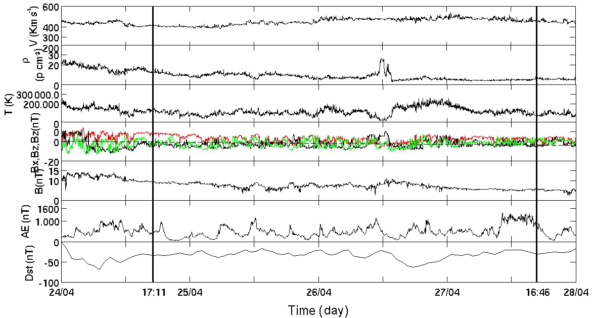
Figure 1 Solar wind parameters and geomagnetic indices during the HILDCAA event occurring from 17:11 UT on 24 April to 16:46 UT on 27 April 1998. From top to bottom, the panels show the solar wind speed; density; temperature; IMF components B_x (red), B_y (black), and B_z (green); the IMF magnitude; the AE index; and the Dst index.

The wavelet transform (WT) applied on f(t) time series is defined as

$$\begin{array}{}\text{(2)}& {\displaystyle }{\displaystyle }\text{TW}(a,b)=\int f\left(t\right){\mathit{\psi }}_{a,b}^{\ast }\left(t\right)\mathrm{d}t,\end{array}$$

where f(t) is a time series, ψ_a,b(t) is the wavelet function, and ${\mathit{\psi }}_{a,b}^{\ast }\left(t\right)$ represents the complex conjugate of the wavelet function ψ_a,b(t).

We used the cross-wavelet transform to obtain the common periods between two time series and, also, to study the temporal variability of the main periods found (Bolzan et al., 2012). The XWT is given by (Grinsted et al., 2004)

$$\begin{array}{}\text{(3)}& {\displaystyle }{\displaystyle }{W}^{yx}(a,b)=W^y(a,b)W^x(a,b{)}^{\ast },\end{array}$$

where W^y and W^x represent the WT applied on the time series y(t) and x(t), respectively, and (^∗) represents the complex conjugate of the transform.

We also used the global wavelet spectrum (GWS) that is used to identify the most energetic periods present on the cross-wavelet analysis. The GWS is given by

$$\begin{array}{}\text{(4)}& {\displaystyle }{\displaystyle }\text{GWS}=\int \mathrm{|}\text{TW}(a,b){\mathrm{|}}^{\mathrm{2}}\mathrm{d}b.\end{array}$$

3.2 Classical cross correlation

The cross correlation between two series provides the degree of similarity between them, along with the displacement between them in time (lag). The correlation between two series, X and Y, is given by

$$\begin{array}{}\text{(5)}& {\displaystyle }{\displaystyle }r={\displaystyle \frac{\sum \left(X_i-\stackrel{\mathrm{‾}}{X}\right)\cdot \sum (Y_i-\stackrel{\mathrm{‾}}{\stackrel{\mathrm{‾}}{Y}})}{\sqrt{\sum (X_i-\stackrel{\mathrm{‾}}{X}{)}^{\mathrm{2}}\sqrt{\sum (Y_i-\stackrel{\mathrm{‾}}{Y}{)}^{\mathrm{2}}}}}},\end{array}$$

where r is the correlation coefficient.

The correlation coefficient defines how well correlated the two series are, varying from −1 to 1. When the correlation coefficient is less than zero it means that the correlation is negative, with −1 being the maximum negative correlation value, known as the perfect negative correlation. When the correlation coefficient is greater than zero, we have the positive correlation, with 1 being the perfect positive correlation. When the correlation coefficient is zero, it means that there is no correlation between the two series.

The classical correlation is calculated by the displacement of one series relative to the other by units of time (t), which provides the lag of the correlation (Davis, 1986).

4 Results

Figure 1 shows the behavior of the solar wind parameters during a HILDCAA event that occurred from 17:11 UT on 24 April to 16:46 UT on 27 April 1998. The HILDCAA interval is marked by two vertical lines. The top panel shows the solar wind speed V. It increases from a value of ∼ 420 to > 530 km s⁻¹ during this interval. The latter represents a HSS. The proton density is shown in the second panel. At the beginning of the event, the density decays from ∼ 15 protons cm⁻³ in the first 7 h to ∼ 7 protons cm⁻³. It keeps oscillating between 7 and 15 protons cm⁻³ until ∼ 08:00 UT on 26 April, when a jump is observed, and the density is enhanced to ∼ 27 protons cm⁻³, followed by a decay, reaching a value of ∼ 4 protons cm⁻³. After this, the density is more or less constant until the end of the event. The third panel presents the solar wind proton temperature that varies from ∼ 2.8 × 10⁴ to ∼ 2.65 × 10⁵ K.

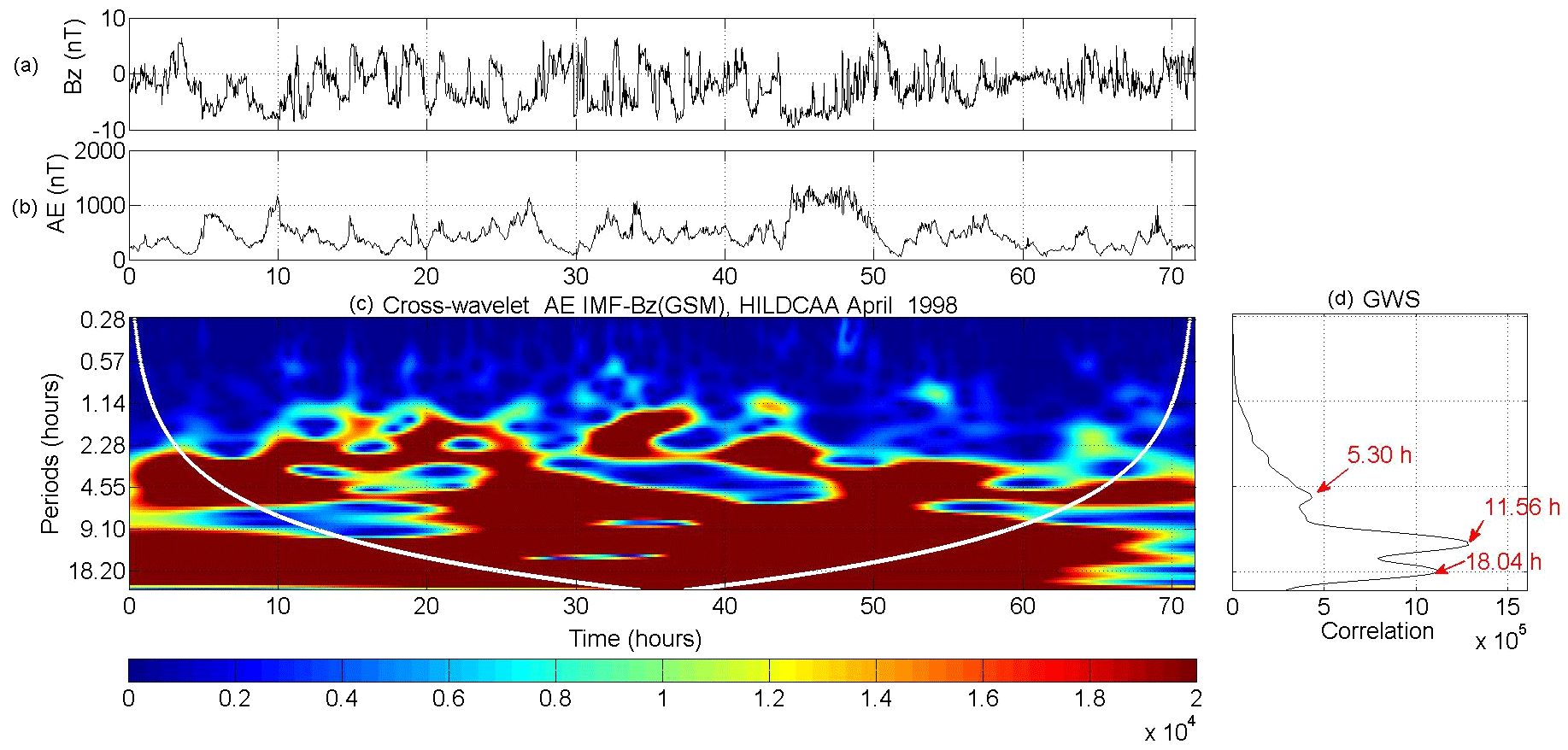
Figure 2 (a) Time series of the IMF B_z component. (b) The AE index. (c) Cross-wavelet spectrum periodogram during the HILDCAA event from 17:11 UT on 24 April to 16:46 UT on 27 April 1998. (d) The global wavelet spectrum shows the main periods of correlation.

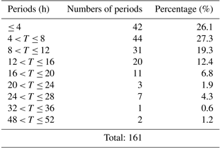
Table 1 Main periods of higher correlation between the IMF B_z component and AE index.

The fourth panel shows the IMF components: B_x (red), B_y (black), and B_z (green). The B_z component exhibits oscillations between −8 and 7 nT, caused by the Alfvén waves. The IMF magnitude (fifth panel) decays in the initial hours and shows some variations until about the 00:00 UT of 27 April. These variations are in the range of 3–11 nT, which are in the range of the typical IMF intensity (5–10 nT) observed near the orbit of the Earth (Baumjohann and Nakamura, 2007).

The AE index (sixth panel) fulfills the HILDCAA criteria. The bottom panel shows the Dst index, which increased slowly from −40 to −20 nT. Particle precipitation in the ring current during the HILDCAA event can be responsible for the slow variations of the Dst index (Soraas et al., 2004).

In order to study the solar-wind–magnetosphere coupling during HILDCAA events, the cross-wavelet analysis was applied to the IMF B_z (considered the cause of events) and to the AE index (consequence). From the GWS results, the distribution of the correlated major periods between these two variables was also studied. In addition to the cross-wavelet analysis, the classical correlation technique was also applied in order to analyze the correlation between those two series and to obtain the time delay (lag) between them.

Figure 2a and b show the temporal variations of the IMF B_z and the AE index, respectively. Figure 2c and d show the cross-wavelet analysis between B_z and AE, as well as the GWS. These are for the HILDCAA event shown in Fig. 1. Three periods of higher correlation can be observed: these are at 5.30, at 11.56, and at 18.04 h (Fig. 2c).

Table 1 shows a summary of the results for all of the 52 HILDCAA events between 1995 and 2011. It was observed that the interval between 4 and 8 h represented most of the periods of highest correlation, with 27.3 %. More than 53 % of the events presented high correlations in periods shorter than 8 h. Further, 85 % of HILDCAAs showed higher cross-correlation power for periods ≤ 16 h.

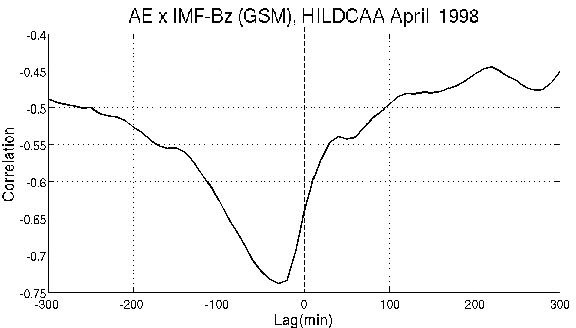
Figure 3 Classical cross correlation between IMF B_z and AE index during the HILDCAA event from 17:11 UT on 24 April to 16:46 UT on 27 April 1998. Maximum cross-correlation coefficient (r = −0.74) is found at a lag = −30 min.

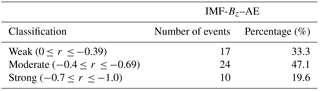
Table 2 Classification and distribution of the classical cross-correlation coefficients between IMF B_z and AE index during HILDCAA events that occurred between 1995 and 2011.

The periods observed here are similar to the periods (< 10 h) of Alfvén waves in the polar region of the Sun (Smith et al., 1995). Among all 52 HILDCAA events studied, only 4 are associated to ICMEs (interplanetary CMEs); the other 48 events are related to CIRs and HSSs. As mentioned earlier, the HSSs emanate from the solar coronal holes and are embedded with Alfvénic fluctuations. Thus, the efficient solar-wind–magnetosphere coupling during the HILDCAAs is associated with the IMF B_z Alfvén fluctuations with southward IMFs leading to the reconnection with the geomagnetic field. This is considered to be the main cause of the HILDCAA-related geomagnetic activity (Tsurutani and Gonzalez, 1987).

As mentioned previously, the classical correlation allows determining the correlation and time lag between two time series. Both the IMF B_z and the AE index had 1 min resolution, but an average of 10 min was used for the calculation of the classical cross correlation, due to the presence of noise observed for an average of 1 min.

Classical cross correlation between B_z and the AE index during the HILDCAA event shown in Fig. 1 is presented in Fig. 3. We can observe that the B_z and AE are highly anticorrelated, with a considerably high correlation coefficient of −0.74 at a time lag of −30 min. This can be interpreted as the response time of the AE index to the perturbations that occurs in the IMF B_z component. The negative correlation coefficient (anticorrelation) occurs because more energy would be transferred from solar wind to the magnetosphere when B_z is more negative, giving as a response a higher AE index. The horizontal axis of Fig. 3 presents the lag between these two time series. We can see that the lag is negative, which occurs because in the computational algorithm used to calculate the correlation between the time series; the AE index was supplied first to the IMF B_z. The positive time lag has no physical meaning, because it would mean that the AE, which is considered to be the geomagnetic consequence, happened before the B_z (cause).

Table 2 presents the cross-correlation results. In this table are shown the correlation classification intervals and the percentage distribution of the events for which the correlation was estimated. The cross correlation was moderate for 47.1 % of the events, for 33.3 % the correlation was weak, and 19.6 % of the events have high correlation. Thus, 66.7 % of HILDCAA events exhibited a moderate–strong correlation (≥ 0.4).

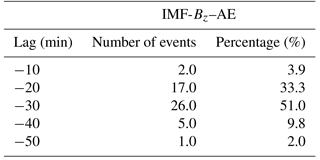
In order to find the best lag where the cross correlation between the two time series is the higher, we applied this procedure for chosen 5 lag intervals. Table 3 shows the 5 lag intervals and the number of events where we obtained the maximum correlation between the AE and IMF B_z of IMF time series. We can see that the lag where we have the maximum number of events was 30 min with 51 % of the events. Furthermore, it is possible to observe that 84.4 % of the events have the lag between −20 and −30 min, which is similar to the value observed by Tsurutani et al. (1990). They reported time lags of 20–25 min during HILDCAAs.

Table 3 Distribution of the intervals of lag between IMF B_z component and the AE index.

Bargatze et al. (1985) studied the relationship between the solar wind and magnetic activity using a solar wind input function and the auroral AL index and observed two pulse peak responses from the magnetosphere in different time lags (20 and 60 min). The peak with a lag of 20 min was associated with magnetospheric activity driven directly by the solar wind coupling. The second pulse, with a lag of 60 min, was related to the magnetospheric activity driven by the release of energy stored in the magnetotail. In the present work, only a lag of 20 min was observed, and no lag of 60 min was found. This result can be explained as follows. During the HILDCAA events the AE index exhibits high values, implying strong geomagnetic and auroral activities. These strong geomagnetic HILDCAA intervals seem to be directly driven, associated with a 20 min time lag as reported by Bargatze et al. (1985). The peak of 60 min is possibly dominant in the case of moderate geomagnetic and auroral activities (not applicable to HILDCAAs).

5 Conclusions

In this work, we studied the solar-wind–magnetosphere coupling during HILDCAA events. We have identified the main periodicities of the IMF B_z and AE index during these events using the cross-wavelet (XWT) analysis, and we also applied the classical cross-correlation analysis to study the correlation and time lag between them.

In the present work, we have shown that the solar-wind–magnetosphere coupling during HILDCAA events is most efficient in periods equal to or shorter than 8 h. These are in the same range as the periodicities observed in the interplanetary Alfvén waves in the HSSs (Smith et al., 1995). This result corroborates the fact that the reconnection between the Alfvénic fluctuations in the IMF B_z and the geomagnetic fields in the magnetopause is the main cause of the HILDCAA events.

Through the classical correlation analysis technique, moderate correlation (0.4–0.7) was obtained between the AE and the IMF B_z. The time lag between them is mostly 20–30 min. This is close to the time lag (20–25 min) reported by Tsurutani et al. (1990). The correlation coefficients between IMF B_z and AE observed in the present work (0.4–0.7) are also consistent with the value (0.62) reported by them. This represents moderate correlation between the geomagnetic activity (AE) index and the interplanetary parameter (IMF B_z).

Thus we may conclude that the solar-wind–magnetosphere coupling during HILDCAAs is mainly due to magnetic reconnection between southward IMF B_z and magnetopause fields. This mechanism is more efficient at periods of 8 h or less, with a 20–30 min time lag between IMF variations and magnetosphere and auroral response.