The geomagnetic coast effect at two 80° S stations in Antarctica, observed in the ULF range

We examined the coast effect in Antarctica along the 80^∘ S magnetic parallel. We used the geomagnetic field measurements at the two coastal stations of Mario Zucchelli Station and Scott Base, and, as a reference, at the inland temporary station Talos Dome, during 18 January–14 March 2008. Spectral analysis in the Pc5 frequency range (1–7 mHz) revealed large differences between coastal and inland stations, such as higher spectral power levels in the vertical component and higher coherence between horizontal and vertical components at coastal stations. Using the interstation method on selected active time intervals, with Talos Dome as a remote reference station, we found that remote reference induction arrows are directed almost perpendicularly with respect to their respective coastlines. Moreover, the single-station analysis shows that at Talos Dome the amplitude of the induction arrows is much smaller than at coastal stations. These results clearly indicate that coast effect at a few hundred kilometers from the coastline is relatively small. The coast effect on polarization parameters was examined, for a Pc5 event that occurred on 11 March 2008. The results evidenced that the azimuthal angle of polarized signals at one of the coastal stations is largely different with respect to the inland station (by ∼ 110^∘), while the polarization ratio and ellipticity attain comparable values. We proposed a correction method of the polarization parameters, which operates directly in the frequency domain, obtaining comparable azimuthal angles at coastal and inland stations.

Keywords. Ionosphere (wave propagation) – magnetospheric physics (polar cap phenomena; storms and substorms)

1 Introduction

Magnetospheric ultra-low-frequency waves (ULF waves, 1.7–5 Hz) driven by the solar wind are successfully studied using geomagnetic field measurements at polar latitudes (Engebretson et al., 2006; De Lauretis et al., 2010; Regi et al., 2015). Such regions are magnetically linked to the regions where the solar wind directly interacts with the geomagnetic field; therefore, they are particularly suitable to investigate the generation of the ULF waves and their propagation in the magnetosphere.

In this context, it is important to exclude contaminations of the signals such as, for example, the effects of the ground conductivity. Waves transmitted from the magnetosphere to the ground can be partially reflected by the ground itself, so that a ground magnetometer measures both the primary source (the magnetospheric waves) and the variations induced by underground electric currents, which represent the secondary source (Parkinson, 1959; Banks, 1973). The efficiency of the reflection increases with increasing conductivity so that, for a perfect horizontal conductor, the vertical field component Z_in induced by the internal currents cancels the external field variations Z_ext. The attenuation of the vertical component and, in addition, an increase of the horizontal component are predicted for a horizontal uniform conducting lamina which is representative of the Earth surface (Parkinson, 1962). The same result is predicted by Price (1950) when a spatially uniform external field induces currents in a half-space of uniform conductivity. It follows that the vertical field $Z=Z_{\mathrm{in}}+Z_{\mathrm{ext}}$ may not be zero if there are nonuniform external fields (Banks, 1973) or nonuniform horizontal ground conductivity (Villante et al., 1998). For example, at a land–sea interface, lateral conductivity gradients cause large Z values, inland from the border of the sea, as for example at observatories on the coastline, since the higher seawater conductivity provides a larger vertical field with respect to the land. In this case, the variation field still lies in a plane, the “Parkinson plane”, which is no longer horizontal but is tilted upward toward the sea (Parkinson and Jones, 1979).

Early investigations in the time domain conducted by Parkinson (1959) evidenced a clear relationship between the vertical and horizontal components due to ground-induced electric currents. The geomagnetic fluctuations, induced by the ground currents, at periods T less than 1 h (or frequencies higher than 0.3 mHz), tend to be confined in the horizontal plane, due to their lower skin depth $D_{\mathrm{ep}}\propto \sqrt{T}$; close to coastlines, the Parkinson's plane tends to be inclined (Gregori and Lanzerotti, 1980; Jones, 1981; Wolf, 1982), probably introducing, on the ground, changes in the polarization pattern of ULF waves in the horizontal plane.

More recently, experimental observations by De Lauretis et al. (2005), conducted in the ULF Pc3 frequency range (22–100 mHz) at the high-latitude stations of Mario Zucchelli (at Terra Nova Bay, TNB) and Concordia (at Dome C, DMC), in Antarctica, showed that azimuthal angles are generally between 45 and 75^∘ at TNB, which is located on the coastline, while they are almost uniformly distributed at DMC, on the Antarctic plateau, far away from the coast.

Moreover, similar results are found at TNB by Regi et al. (2017) in the Pc1–2 frequency range (100–500 mHz). These results indicate that the signal power at TNB tends to be higher along the east–west magnetic component. As suggested by De Lauretis et al. (2005), the polarization characteristics may be affected by ground conductivity anomalies, due to the closeness of TNB to the coast.

The availability of simultaneous measurements from observatories at TNB and Scott Base (SBA; data provided by INTERMAGNET database), allows us to make an interesting comparison, in that the stations are located approximately at the same geomagnetic latitude (∼ 80^∘ S), although near different coastlines. As pointed out by Schmucker (1970) and Viljanen et al. (1995) (see also Fujiwara and Tou, 1996; Beamish, 1982; Vujić and Brkić, 2016), a suitable analysis in both vertical and horizontal components can be assessed by using a reference station, which should be ideally far away from the ground anomalies (i.e., from the coast). In this regard, we used as a reference station the temporary installation at Talos Dome (TLD, ∼ 80^∘ S), deployed during the 2007–2008 Antarctic campaign at ∼ 270 and 560 km from TNB and SBA, respectively, and operating during 18 January–14 March 2008 (Lepidi et al., 2017).

Our statistical investigation shows that, in the frequency range 1–7 mHz (Pc5 waves), the geomagnetic field measurements at TNB and SBA are contaminated by the coast effect, clearly identified by the induction vectors, which point almost perpendicularly to the respective nearest coastlines. Moreover, by examining a Pc5 case event, we observed different polarization characteristics in the horizontal geomagnetic field variations at TNB and TLD, which can be due to the closeness of TNB to the coastline, as suggested by De Lauretis et al. (2005).

2 Data analysis and methods

Geomagnetic field variations were measured at the three sites by means of three-axis fluxgate magnetometers along the northward (H), eastward (D), and vertically downward (Z) directions in the geomagnetic reference frame. For this analysis we used data sampled at 1 min in the time interval 18 January–14 March 2008, and the horizontal components of the geomagnetic field were conveniently rotated along the northward (X) and eastward (Y) direction in the geographic reference frame. Geomagnetic field variations at SBA were directly provided in the geographic reference frame, in the INTERMAGNET database. At TNB the rotated components X and Y were computed using the measured value of the declination ${\mathit{\delta }}_{\mathrm{0}}=\mathrm{135}{}^{\circ }{\mathrm{44}}^{\prime }$ (IGRF ${\mathit{\delta }}_{\mathrm{0}}=\mathrm{135}{}^{\circ }{\mathrm{45}}^{\prime }$) and the horizontal field intensity H₀=8050 nT (IGRF H₀=7680 nT), while at TLD, ${\mathit{\delta }}_{\mathrm{0}}=\mathrm{137}{}^{\circ }$ and H₀=6670 nT were obtained from the IGRF model. Such frequency sampling allows us to study ULF waves up to a frequency of 8.33 mHz. Before spectral analysis, each time series was high-pass filtered by removing long period fluctuations, such as S_q variations, by using the 1 min moving-average procedure over 3 h windows. We computed 3 h nonoverlapping power spectra by means of Welch's method on three 1 h subintervals, with a frequency resolution of ∼0.27 mHz. Spectra and cross-spectra were frequency smoothed by using a 5-point triangular window, so that the final frequency resolution is ∼ 0.83 mHz (De Lauretis et al., 2010).

The geomagnetic anomalies are investigated in the frequency domain. The ground conductivity anomaly effect on vertical component can be estimated by means of the following empirical relationship (Parkinson and Jones, 1979):

$$\begin{array}{}\text{(1)}& \mathrm{\Delta }{Z}_{\mathrm{s}}\left(f\right)=A_{\mathrm{s}}\left(f\right)\mathrm{\Delta }{X}_{\mathrm{s}}\left(f\right)+B_{\mathrm{s}}\left(f\right)\mathrm{\Delta }{Y}_{\mathrm{s}}\left(f\right),\end{array}$$

which represents the induction effects on vertical component from the horizontal field variations at a geomagnetic station (single-station analysis). In this formula, where f indicates the frequency, the induction effects on the horizontal components are negligible (i.e., ΔX_s(f) and ΔY_s(f) are the normal field variations).

The contribution of anomalies to the vertical and horizontal geomagnetic field can be estimated by using the so-called interstation transfer functions (Schmucker, 1964; Beamish, 1982; Fujiwara and Tou, 1996; Vujić and Brkić, 2016; Harada et al., 2005). Let us assume the following:

• the normal field variation ΔB_n(t), produced by the primary field and by the inducted secondary field due to normal conducting ground, is measured at a reference station not affected by ground anomaly, so that ΔB_n(t)=ΔB_r(t) (t indicates the time);

• the anomalous part ΔB_a(t), that includes only contributions from lateral discontinuities in geoelectric structures, is related with the normal field through the linear relationship between Fourier transforms ΔB_a(f)=MΔB_r(f).

From Schmucker (1970) the Fourier transform of geomagnetic field fluctuations resulting at the anomalous site can be expressed at a given frequency by $\mathrm{\Delta }{\mathbf{\text{B}}}_{\mathrm{s}}\left(f\right)=\mathrm{\Delta }{\mathbf{\text{B}}}_{\mathrm{r}}\left(f\right)+\mathbf{\text{M}}\mathrm{\Delta }{\mathbf{\text{B}}}_{\mathrm{r}}\left(f\right)+\mathit{\delta }\mathbf{\text{B}}\left(f\right)$, where δB is the error vector and M represents the induction tensor (3 by 3 matrix at a given frequency) whose elements represent transfer functions.

Fujiwara and Toh (1996) and Beamish (1982) further simplified the linear system, assuming a negligible ΔZ_r, yielding to

$$\begin{array}{}\text{(2)}& \left[\begin{array}{c}\mathrm{\Delta }{X}_{\mathrm{s}}\\ \mathrm{\Delta }{Y}_{\mathrm{s}}\\ \mathrm{\Delta }{Z}_{\mathrm{s}}\end{array}\right]=\left[\begin{array}{cc}C+\mathrm{1}& D\\ E& F+\mathrm{1}\\ A& B\end{array}\right]\left[\begin{array}{c}\mathrm{\Delta }{X}_{\mathrm{r}}\\ \mathrm{\Delta }{Y}_{\mathrm{r}}\end{array}\right]+\left[\begin{array}{c}\mathit{\delta }{X}_{\mathrm{r}}\\ \mathit{\delta }{Y}_{\mathrm{r}}\\ \mathit{\delta }{Z}_{\mathrm{r}}\end{array}\right].\end{array}$$

The transfer functions A, B, C+1, D, E and F+1 of tensor M can be estimated as in Everett and Hyndman (1967) (see also Banks (1973) and Fujiwara and Tou (1996) for detailed formulas and different estimation methods).

In the present study we estimated the transfer functions by means of the least-square method over N spectra as in Everett and Hyndman (1967).

It is worth noting that the errors in transfer functions are negligible because they are reduced by a factor $\mathrm{1}/\sqrt{N}$, as we found in a separate analysis by means of a Monte Carlo test. The third line of Eq. (2) relates the horizontal fluctuations at the reference site with the vertical fluctuations at the anomalous site:

$$\begin{array}{}\text{(3)}& \mathrm{\Delta }{Z}_{\mathrm{s}}\left(f\right)=A\left(f\right)\mathrm{\Delta }{X}_{\mathrm{r}}\left(f\right)+B\left(f\right)\mathrm{\Delta }{Y}_{\mathrm{r}}\left(f\right).\end{array}$$

A second set of equations (from Eq. 2) relates the fluctuations of the horizontal field at reference and anomalous sites

$$\begin{array}{}\text{(4)}& \left[\begin{array}{c}\mathrm{\Delta }{X}_{\mathrm{s}}\\ \mathrm{\Delta }{Y}_{\mathrm{s}}\end{array}\right]=\left[\begin{array}{cc}C+\mathrm{1}& D\\ E& F+\mathrm{1}\end{array}\right]\left[\begin{array}{c}\mathrm{\Delta }{X}_{\mathrm{r}}\\ \mathrm{\Delta }{Y}_{\mathrm{r}}\end{array}\right]+\left[\begin{array}{c}\mathit{\delta }{X}_{\mathrm{r}}\\ \mathit{\delta }{Y}_{\mathrm{r}}\end{array}\right],\end{array}$$

while Eq. (1) is applicable to a single station, the Eqs. (2)–(4) refer to the interstation method. By equating Eq. (1) and (3) and using the relationships (4), we obtain the remote reference transfer functions (Fujiwara and Toh, 1996):

$$\begin{array}{}\text{(5)}& A_{\mathrm{r}}={\displaystyle \frac{A(F+\mathrm{1})-BE}{(C+\mathrm{1})(F+\mathrm{1})-DE}},\end{array}$$

$$\begin{array}{}\text{(6)}& B_{\mathrm{r}}={\displaystyle \frac{B(C+\mathrm{1})-AD}{(C+\mathrm{1})(F+\mathrm{1})-DE}},\end{array}$$

which represent the transfer functions A_s and B_s, obtained using the horizontal variations at the reference station.

At a given station, through the complex coefficients A_r and B_r, we can define the induction arrow; the real part (ℜ) of transfer functions describes the in-phase response, while the quadrature response is defined by the imaginary part (ℑ), which is generally characterized by a smaller amplitude and unclear behavior. The reversed real induction arrow points towards the anomaly (Wiese, 1962; Viljanen et al., 1995).

The interstation analysis allows us to estimate the normal field fluctuations, in the frequency domain. Assuming that interstation transfer functions of horizontal components are known, by inverting the Eq. (4), and taking into account that ΔX_r=ΔX_n and ΔY_r=ΔY_n, the normal signal can be estimated as follows:

$$\begin{array}{}\text{(7)}& \left[\begin{array}{c}\mathrm{\Delta }{X}_{\mathrm{n}}\\ \mathrm{\Delta }{Y}_{\mathrm{n}}\end{array}\right]={\left[\begin{array}{cc}C+\mathrm{1}& D\\ E& F+\mathrm{1}\end{array}\right]}^{-\mathrm{1}}\left[\begin{array}{c}\mathrm{\Delta }{X}_{\mathrm{s}}\\ \mathrm{\Delta }{Y}_{\mathrm{s}}\end{array}\right].\end{array}$$

Although useful, the above technique requires caution in computing the transfer functions. Indeed, this method fails if the plane wave assumption is not valid (Viljanen et al., 1995 and reference therein). Plane-wave events at high latitudes can be characterized by the following:

• a high correlation of the horizontal components at different stations (i.e., between TLD and coastal stations of TNB and SBA);

• a low coefficient $U=\mathrm{100}\mathit{\sigma }({\mathit{\chi }}_{\mathrm{s}}-{\mathit{\chi }}_{\mathrm{r}})/max\left(\right|{\mathit{\chi }}_{\mathrm{r}}\left|\right)$ (%), where σ(χ_s−χ_r) indicates the standard deviation of the difference between field measurements ($\mathit{\chi }=X,Y$) at anomalous and reference stations (see Viljanen et al., 1995 for details). U=0 corresponds to a uniform field.

Moreover, the transfer function formulas have a common dependence on $\mathrm{1}/(\mathrm{1}-{\mathit{\gamma }}^{\mathrm{2}}$), as shown in Eq. (2) of Jones (1981), where γ² represents the magnitude squared coherence between horizontal components at a reference site (X_r and Y_r if interstation method is used; Eqs. (4)–(9) in Fujiwara and Tou, 1996), or at any site (X_s and Y_s if single-station method is used; Sect. 3.1 in Everett and Hyndman, 1967). In order to avoid instability in transfer functions, we selected only events showing a maximum coherence of 0.6 (this threshold is sufficiently lower than 1 but is still high enough to select a significant number of events).

Table 1 Geographic coordinates, IGRF08 corrected geomagnetic coordinates and time in UT of the geomagnetic local noon for the three stations.

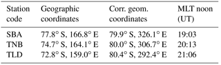
Figure 1 The position of the geomagnetic stations. Dashed lines mark geomagnetic coordinates.

We used TLD as the reference station, since our analysis demonstrated that it is poorly affected by coast effects; the station is located in the inner Antarctic region (∼ 270 km from TNB and ∼ 560 km from SBA). The three stations are approximately at the same geomagnetic latitude of ∼ 80^∘, and are located in the polar cap but approach the dayside cusp and related phenomena around local magnetic noon; SBA, TNB and TLD are approximately equispaced by 1 h in magnetic local time (MLT; see Table 1 and Fig. 1). Due to the larger distance from TLD, SBA should reveal a lower correlation with TLD than TNB.

3 Experimental results

In Sect. 3.1 we present the spectral characteristics at the three stations. In Sect. 3.2 we show the transfer functions resulting from the interstation technique, for vertical and horizontal components, also showing single-station induction arrows (SSIAs) and remote reference induction arrows (RRIAs) at TNB and SBA. Finally, in Sect. 3.3 we investigated the anomalous polarization azimuthal angle observed at TNB during a Pc5 event that occurred on 11 March 2008.

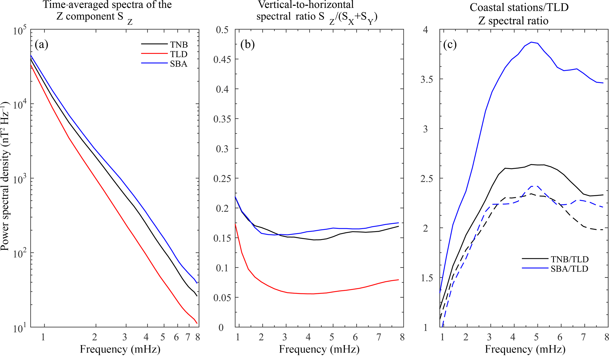
Figure 2 Average spectral density of the Z component (a) and spectral ratio $Z/(X+Y)$ (b) at each geomagnetic station; spectral ratio of the Z components at each coastal station and at TLD (c; dashed lines during disturbed magnetospheric conditions).

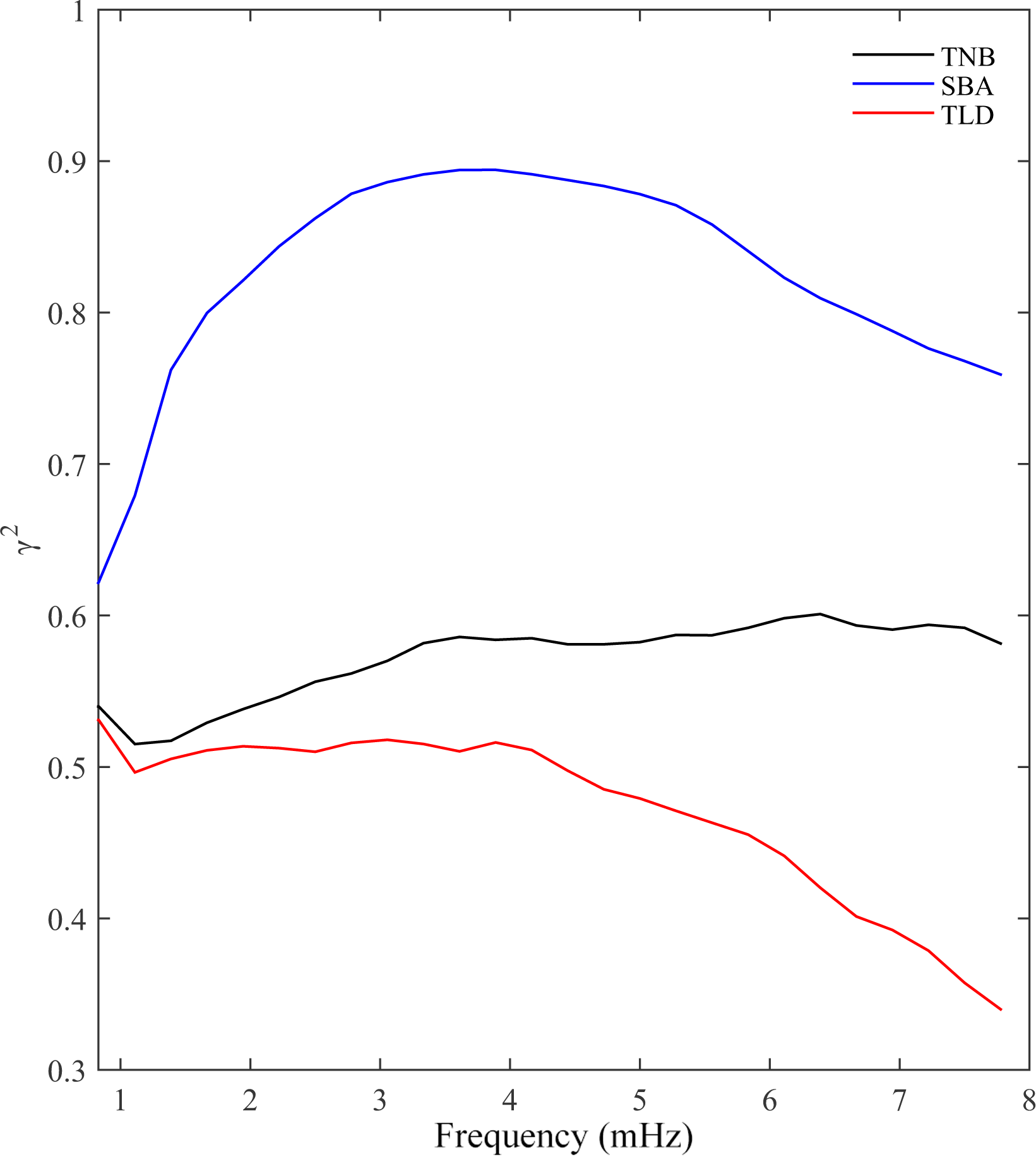
Figure 3 Average multiple coherence between vertical and horizontal components for inland (red line) and coastal (black and blue lines) ground stations.

3.1 Power spectra ratio at coastal and inland stations

We found that the spectral power on the Z component at TLD shows a different level with respect to the stations on the coast which, on the contrary, are characterized by a similar behavior.

Figure 2 shows the time-averaged power spectral density (PSD) of the Z component (S_Z) (panel a), the spectral ratio (SR) between Z and the horizontal X and Y components ($S_Z/(S_X+S_Y)$ at each station (panel b), and the ratio between S_Z at coastal stations and S_Z at TLD (panel c). We found that the average S_Z is higher at TNB and SBA than at TLD and the difference increases with increasing frequency. The SR value is much lower than 1 at all stations, as expected for the conductive ground; however, it is much higher at the coastal stations with respect to TLD and similar at TNB and SBA. Moreover, the ratio between S_Z at coastal stations and S_Z at TLD is higher than 1 at both stations, with larger values at SBA, particularly for frequencies >2 mHz. This aspect will be further discussed later, in the next section.

The clear difference between spectral behaviors at coastal stations with respect to the inland station suggests that at TNB and SBA the ULF fluctuations, at frequencies in the range 0.3–8 mHz, can be affected by the high conductivity of the seawater.

Evidence of a possible relationship between the vertical and horizontal field variations at each station can be revealed by estimating the multiple coherence γ² between such components (Bendat and Piersol, 1971). Figure 3 shows the time-averaged γ² at the three stations, by assuming horizontal components as inputs and the vertical component as output. In the examined frequency range, the coherence is higher at the coastal stations than at TLD, where the vertical and horizontal variations seem to be poorly related, especially at frequencies >4 mHz.

These results suggest that the geomagnetic field measured at TLD station is the normal field, unaffected by ground anomalies, so TLD can be adopted as a reference station.

It is worth noting that the differences between the coastal stations and the inland station tend to decrease with decreasing frequency, probably due to both the effects of a horizontally homogeneous deep lithosphere under all geomagnetic stations (i.e., also under the sea), which responds to the low frequencies, and the effects of uniform-inducing ULF waves at all ground stations, since at low frequencies the wavelengths (several Earth radii) are larger than the maximum distance between stations (∼ 600 km).

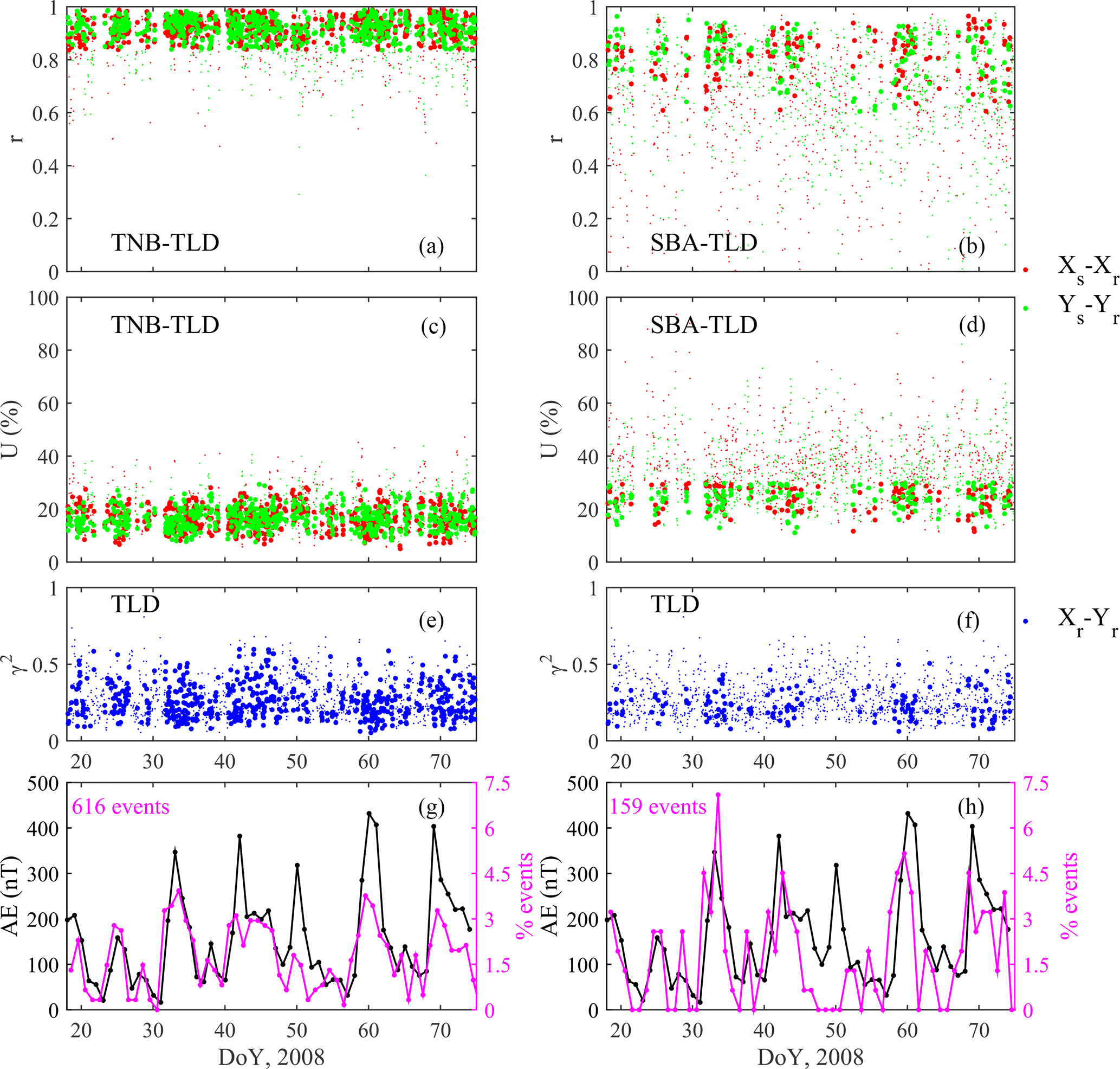
Figure 4 First and second row: r and U coefficients for the pair TNB–TLD (a, c) and SBA–TLD (b, d) for the whole data set; plane-wave events are marked by heavy dots. Third row: coherence between the horizontal X and Y components at TLD for TNB and SBA events (e, f, respectively); selected events are marked by heavy dots. Fourth row: comparison between the daily number (%) of selected events (pink line) and the daily AE index (black line), for the pair TNB–TLD (g) and SBA–TLD (h).

3.2 Vertical and horizontal transfer functions using the interstation analysis

To apply the interstation technique, we need to satisfy two requirements, as explained in Sect. 2: the source should be a common plane wave simultaneously observed at coastal and reference stations, and the coherence between horizontal components at the reference station should be sufficiently low.

Figure 4 shows the correlation coefficient r (panels a and b) and the deviation from uniformity U (panels c and d) of the horizontal components at the pair TNB–TLD (on the left) and SBA–TLD (on the right) for the whole data set. Plane-wave events are assumed if r is higher than 0.8 at TNB and 0.6 at SBA, and U is below 30 % at each station. The number of plane-wave events is ∼ 600 and ∼ 160 at TNB and SBA, respectively. The smaller number at SBA with respect to TNB (even using a lower threshold for r) is probably due to the larger distance of SBA from TLD. Moreover, panels e and f show the coherence between the horizontal X and Y components at TLD for the plane-wave events at TNB and SBA; we selected only the plane-wave events in which the coherence is lower than 0.6. The selected events occurred mostly during high geomagnetic activity, as can be seen from the comparison between the percentage of selected events and the AE index for each day (bottom panels). The percentage is computed with respect to the total number of selected events.

Figure 5 The coherence between horizontal homologous components at reference and coastal stations as a function of frequency. The horizontal bar indicates the 99 % confidence level.

In order to take into account only clear events generated during disturbed geomagnetic conditions, we restricted our analysis to events corresponding to AE higher than 50 nT. In this case, the spectral ratio between the Z components at coastal stations and TLD becomes similar (as can be seen in Fig. 2c, dashed lines). This suggests that we observe a similar effect at the two coastal stations.

For the selected events we examined the coherence between homologous components at reference and each coastal station. Figure 5 shows the median values of the coherence at the two stations. It can be seen that the horizontal signals appear significantly coherent at the TNB–TLD pair (particularly at frequencies <5 mHz; panels a and c), more than at the SBA–TLD pair (panels b and d), probably due to the larger distance of SBA from TLD.

Figure 6 Remote reference transfer functions A_r and B_r at TNB (a, b) and SBA (c, d); solid and dotted lines indicate the real and imaginary parts, respectively.

Figure 7 Single-station induction arrows at SBA, TNB and TLD (a, c) and remote reference induction arrows at SBA and TNB using TLD as a reference geomagnetic station (b), obtained from the real part of transfer functions. Geographic parallels and meridians are shown.

Figure 8 Horizontal transfer functions from interstation method at TNB (a, b, c, d) and SBA (e, f, g, h); solid and dotted lines indicate the real and imaginary parts, respectively.

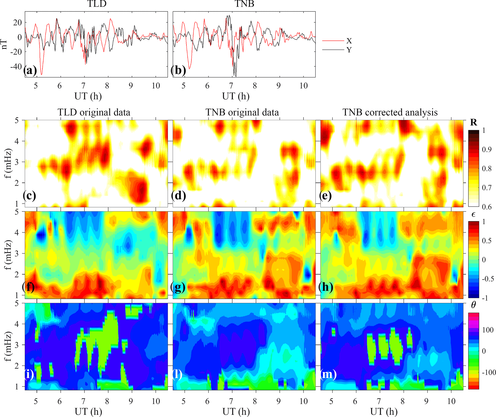
Figure 9 (a, b) Band-pass-filtered time series of the original horizontal components at TNB and TLD for the examined event; (c, d, f, g, i, l) polarization parameters from the original horizontal components at TLD and TNB; (e, h, m) polarization parameters using the interstation method correction procedure at TNB.

Real and imaginary parts of the estimated remote reference transfer functions A_r and B_r are shown in Fig. 6 as a function of frequency. The values of the imaginary parts are very low, close to zero. The real parts of A_r and B_r have a similar level at TNB (panels a and b), while at SBA (panels c and d) larger values are observed in A_r, suggesting that the induced vertical field at TNB is a combination of the inducing horizontal fields, while at SBA, the major source is represented by the fluctuations along the X northward component.

The estimated RRIAs at TNB and SBA are shown, using the stereographic projection, in panel (b) of Fig. 7 for each frequency band (indicated in the color scale), together with the average RRIA (red arrows) computed as

$$\begin{array}{}\text{(8)}& 〈\mathbf{\text{I}}〉={\displaystyle \frac{\mathrm{1}}{N_{\mathrm{f}}}}\sum _{i=\mathrm{1}}^{N_{\mathrm{f}}}{\mathbf{\text{I}}}_{\mathrm{i}},\end{array}$$

where N_f is the number of frequency bands which satisfy the condition γ²>0.5 (from Fig. 5), and I_i are the real part of the induction arrow at the ith-frequency band. In Fig. 7, for a comparison, we also show the SSIAs (panels a and c); at TLD the arrows exhibit a small amplitude and are randomly oriented. It can be seen that the two different methods provide similar results at TNB and SBA, consistent with Fujiwara and Tou (1996), with the respective arrows pointing almost perpendicularly to the nearest coastline.

Regarding the horizontal transfer functions at TNB and SBA, we show the real and imaginary parts of each transfer function (Eq. 4) in Fig. 8. It can be seen that only the values of the real part of the C+1 and F+1 transfer functions are appreciably different from zero for frequencies lower than ∼5 and ∼2 mHz at TNB (panels a, b, c and d) and SBA (panels e, f, g and h), respectively; they relate the anomalous induced field ΔX_a, ΔY_a with ΔX_r and ΔY_r observed at the reference station.

3.3 Polarization analysis using the interstation method correction procedure: a case study of the 11 March 2008 Pc5 event

In order to study the polarization characteristics due to coast effects, we estimated ΔX_n and ΔY_n, from Eq. (7), during a period characterized by high Pc5 activity. We selected the event on 11 March 2008 (Lepidi et al., 2017) and compared the polarization patterns at TLD and TNB. The azimuthal angle θ, the polarization ratio R and ellipticity ϵ were examined on the basis of Fowler et al. (1967) polarization analysis, performed using a moving window of 2 h with a step size of 1 min. For each time window the Welch's method on subwindows of 60 min was used in order to compute spectra and cross-spectra of horizontal fluctuations; each resulting spectrum was smoothed over 5 frequency bands (final frequency resolution of ∼ 0.83 mHz): the averaging and smoothing procedures increase the reliability of the polarization parameters (Bendat and Piersol, 1971; Fowler et al., 1967). Due to the higher distance of SBA from TLD and lower reliability of related transfer functions, in this section we present only the TNB–TLD comparison and discuss frequencies lower that ∼5 mHz, for which anomalous induction effects are significant, as shown in previous sections.

Figure 9 shows the dynamic polarization parameters obtained from the original data at TLD and TNB; the band-pass-filtered time series are shown in panels (a) and (b), respectively. It can be seen that polarization parameters R (panels c and d) and ϵ (panels f and g) are similar; conversely, the azimuthal angle at TNB (panel l) generally differs from TLD (panel i) by ∼ 110^∘, particularly in correspondence to polarized (R>0.8 at TLD) Pc5 fluctuations, i.e., during ∼ 06:30–08:30 UT and in the frequency range 2–4 mHz. The results of the polarization analysis, conducted using data corrected for the coast effect (Eq. 7), are shown in the right-hand-side panels of Fig. 9. It can be seen that the polarization ratio and ellipticity do not change significantly (panels e and h, respectively), while the azimuthal angle at TNB varies in agreement with TLD (panel m).

This example clearly shows that the polarization characteristics (more evident in the azimuthal angle in this case study) may be affected by ground conductivity anomalies, probably due to the closeness of TNB to the coastline, as suggested by De Lauretis et al. (2005) and also observed by Regi et al. (2017) in the higher Pc1–2 frequency range and evidenced by the interstation induction arrows at coastal stations.

4 Conclusions

In the present work we studied the coast effect at the Antarctic geomagnetic stations TNB and SBA during 18 January–14 March 2008, also using the inland temporary station TLD, more than 200 km from the coast, as a reference station. The spectral analysis, in the Pc5 frequency range, revealed a significant difference between coastal and inland stations.

In particular, the Pc5 power of the vertical component at the coastal stations is higher than at the reference station, and the spectral ratio between vertical and horizontal components is similarly high. Moreover, the multiple coherence of the horizontal components with the vertical component reveals higher values at SBA and TNB with respect to TLD. These results suggest that the sea–land interface affects measurements at coastal stations, and confirms TLD as a suitable reference station, since the amplitude of the induction arrows is generally 20 times smaller than at coastal stations, in agreement with Hitchman et al. (2000) and Vujić and Brkić (2016) observations at lower latitudes.

We proposed a method for estimating directly, in the frequency domain, the normal field variations at coastal stations, by inverting the linear relationship between horizontal field measurements at coastal and reference stations. As an example, we showed the Pc5 event on 11 March 2008, for which we observed different azimuthal angles at TNB and TLD. When corrected by means of our method, the azimuthal angle at TNB changes, becoming similar to the angle at TLD, while the polarization ratio and ellipticity do not change significantly. These results indicate that the azimuthal angle of polarized ULF waves at the coastal station of TNB is probably affected by horizontal ground conductivity anomalies, attributable to the sea saltwater, as suggested by De Lauretis et al. (2005).

Most of the geomagnetic stations installed in Antarctica are situated close to the sea, and so geomagnetic measurements could be affected by local coast effects. This work can be regarded as a useful reference in order to remove local effects: for example, without considering coast effects, a comparison between polarization parameters at coastal and inland stations could be misleading, leading to incorrect conclusions. In addition, the spectral techniques shown here could be used not only to study anomalous variations at coastal stations, where the anomaly is persistent, but also to detect possible anomalous effect due to sporadic changes in ground conductivity.