the Creative Commons Attribution 4.0 License.
the Creative Commons Attribution 4.0 License.
 | 29 Jan 2018
Depth of origin of ocean-circulation-induced magnetic signals
Christopher Irrgang
Jan Saynisch-Wagner
Maik Thomas
As the world ocean moves through the ambient geomagnetic core field, electric currents are generated in the entire ocean basin. These oceanic electric currents induce weak magnetic signals that are principally observable outside of the ocean and allow inferences about large-scale oceanic transports of water, heat, and salinity. The ocean-induced magnetic field is an integral quantity and, to first order, it is proportional to depth-integrated and conductivity-weighted ocean currents. However, the specific contribution of oceanic transports at different depths to the motional induction process remains unclear and is examined in this study. We show that large-scale motional induction due to the general ocean circulation is dominantly generated by ocean currents in the upper 2000 m of the ocean basin. In particular, our findings allow relating regional patterns of the oceanic magnetic field to corresponding oceanic transports at different depths. Ocean currents below 3000 m, in contrast, only contribute a small fraction to the ocean-induced magnetic signal strength with values up to 0.2 nT at sea surface and less than 0.1 nT at the Swarm satellite altitude. Thereby, potential satellite observations of ocean-circulation-induced magnetic signals are found to be likely insensitive to deep ocean currents. Furthermore, it is shown that annual temporal variations of the ocean-induced magnetic field in the region of the Antarctic Circumpolar Current contain information about sub-surface ocean currents below 1000 m with intra-annual periods. Specifically, ocean currents with sub-monthly periods dominate the annual temporal variability of the ocean-induced magnetic field.
Keywords. Electromagnetics (numerical methods) – geomagnetism and paleomagnetism (geomagnetic induction) – history of geophysics (transport)
- Article
(13429 KB) - Full-text XML
- BibTeX
- EndNote


The Earth's magnetic field consists of various constituents that are generated and interact with each other on different spatial and temporal scales. The oceanic constituent is induced by the movement of electrically conductive seawater through the geomagnetic core field. During this motional induction process, electric currents are generated in the ocean, which, in turn, induce weak magnetic signals in the range of a few nanotesla (nT). The ocean-induced magnetic field is primarily proportional to conductivity-weighted and depth-integrated water transports (Sanford, 1971). Thus, measurements of oceanic motional induction enable the highly promising possibility to indirectly observe global oceanic transports of water, heat, and salinity.
Following the theoretical foundation of electromagnetic (EM) induction in the ocean (see, e.g., Larsen, 1968; Cox, 1981; Chave, 1983; Chave and Luther, 1990), the focus was shifted towards the numerical modelling of this process. Among others, Stephenson and Bryan (1992), Flosadóttir et al. (1997), Tyler et al. (1997), Vivier et al. (2004), and Manoj et al. (2006) examined the numerical modelling of motional induction due to the general ocean circulation. Along with the prospect of space-borne observations of the ocean-circulation-induced magnetic field from the European Space Agency's (ESA) Swarm mission (Friis-Christensen et al., 2006), Irrgang et al. (2017) demonstrated that such observations can be used to correct an ocean general circulation model in a data assimilation twin experiment.
In previous studies, the oceanic EM current source was usually derived from the conductivity-weighted and depth-integrated ocean velocities. While this is a reasonable approach for most applications, the actual contribution to motional induction from oceanic transports at individual depths of the ocean basin is invisible. However, depth-dependent processes and properties – e.g. baroclinic ocean currents, overturning circulation, friction effects, or ocean bathymetry – have considerable impacts on oceanic electric currents at different depths in the ocean basin. So far, the depth-varying proportion of ocean currents to the signal strength and spatial distribution of EM induction due to the general ocean circulation has not yet been investigated (see also the reviews of Kuvshinov, 2008; Minami, 2017). Nevertheless, this knowledge would be a valuable contribution for the ongoing efforts to infer information about the ocean by observing its emitted magnetic field. In particular, space-borne observations of the ocean-circulation-induced magnetic field, once available, could be related to the underlying large-scale ocean dynamics in a much more precise way than previously assumed.
In this study, we investigate the depth of origin of the ocean-circulation-induced magnetic field. For this, a general ocean circulation model and a three-dimensional EM induction model are used. In particular, the goals are (1) to examine, whether the motional induction process is dominated by thin and fast (near-)surface currents or by slow and massive deep currents, and (2) to outline new applications and limitations of potential observations of motional induction in the context of ocean modelling. The model setups and their combination are described in Sect. 2.1 and 2.2. The experiment design of this study is described in Sect. 2.3. The results are presented in Sect. 3.1 and 3.2. Subsequent implications are discussed in Sect. 3.3. A summary and concluding remarks are given in Sect. 4.
2.1 Ocean general circulation model
The Ocean Model for Circulation and Tides (OMCT; Thomas et al., 2001) is used in this study to simulate the global wind- and buoyancy-driven ocean circulation. The model calculates three-dimensional fields of zonal (u), meridional (v), and vertical (w) ocean velocities, heat (T), and salinity (S), which provide the source for the oceanic EM induction. The global distribution of electric seawater conductivity (σ) is derived from OMCT heat and salinity distributions as described by Irrgang et al. (2016a). Along with the model's wide range of applications (e.g. Dobslaw and Thomas, 2007; Dobslaw et al., 2013; Saynisch et al., 2014), it also has been recently used in combination with different EM induction models (e.g. Saynisch et al., 2016; Irrgang et al., 2016b, 2017).
OMCT is a baroclinic numerical ocean model based on non-linear balance equations for momentum, the continuity equation, and conservation equations for salt and heat. Additionally, the hydrostatic and the Boussinesq approximations are included. The method of Greatbatch (1994) is used to correct artificial mass changes due to the Boussinesq approximation. In this study, we use an OMCT configuration with a horizontal grid resolution of 1∘, 20 vertical z-level layers, and a 20 min time step (Dobslaw et al., 2013). Ocean tides are not included in this setup. OMCT is forced with wind stress, precipitation, evaporation, and surface pressure from reanalysis products of the European Centre for Medium-Range Weather Forecasts (ECMWF; Dee et al., 2011).
The generation of electric currents j due to the moving and conducting seawater in presence of the ambient geomagnetic field is given by Ohm's law,
where is the ocean velocity vector and is the geomagnetic core field. The conductivity-weighted ocean velocities (σu) are the source for oceanic electric currents. To account for electric currents in the whole water column, the conductivity-weighted ocean velocities are integrated from the ocean bottom (−H) to sea surface height (SSH), which yields
at time t with longitudinal, latitudinal, and vertical coordinates . The oceanic electric currents are subsequently calculated by combining Eqs. (1) and (2), namely
and are used as sources for the EM induction model.
2.2 EM induction model
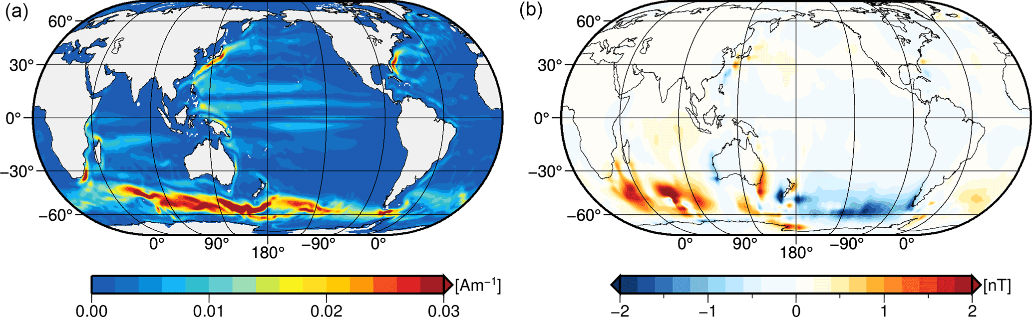
Figure 1(a) Annual mean oceanic electric current density j of the year 2014. (b) Corresponding radial part of the annual mean ocean-induced magnetic field at sea surface.
In this study, we use the three-dimensional (3-D) EM induction model X3DG of Kuvshinov (2008). The model solves Maxwell's equations in frequency domain with a volume integral equation method that utilizes a Green's function technique (see also Kuvshinov and Semenov, 2012; Kelbert et al., 2014). The Earth's electrical conductivity structure is included as a spherical layer of laterally varying surface conductance and an underlying radially symmetric mantle conductivity. The surface conductance layer accounts for the conductivity of the ocean and of underlying sediments. The ocean conductance is derived from a realistic 3-D distribution of annual mean seawater conductivity, which is calculated from OMCT heat and salinity distributions (Irrgang et al., 2016a). The conductance of sediments underneath the oceanic layer is included by combining global sediment thicknesses from Laske and Masters (1997) with respective values for sediment conductivity as described by Everett et al. (2003). The vertical structure of the mantle conductivity follows the results of Püthe et al. (2015). Based on the Earth's electrical conductivity and the oceanic electric currents j (as described in Sect. 2.1), the EM induction model is used to calculate the corresponding ocean-induced magnetic field (see Fig. 1). In particular, we focus on the radial part of the ocean-induced magnetic field, which is emitted outside of the ocean and calculated at both sea surface height and at Swarm satellite altitude (430 km above the sea surface).
2.3 Experiment design

Figure 2Vertical two-layer partition of the oceanic electric current source in scenarios A to D. Values around the separation lines are upper and lower layer thicknesses. Oceanic electric currents in the grey-shaded lower layers are excluded in the scenarios A to D. The reference includes oceanic electric currents from the entire water column.
OMCT is used to simulate the general ocean circulation of the year 2014, which is the basis for the EM induction process in this experiment. The corresponding oceanic electric currents are calculated as described in Sect. 2.1 and instantaneous values are stored with a 5-day sampling. Thus, also the output of the EM induction model has an effective temporal resolution of 5 days. The geomagnetic core field is taken from the International Geomagnetic Reference Field (IGRF-12) and assumed constant during the simulation period, which is reasonable for a simulation period of 1 year (Thébault et al., 2015). The annual mean ocean-induced magnetic field is calculated from the annual mean oceanic electric currents as described in Sect. 2.2 and serves as a reference in this experiment (Fig. 1 and yellow bar in Fig. 2).
In contrast to thin-sheet (2-D) EM induction models (see, e.g., Stephenson and Bryan, 1992; Tyler et al., 1997; Vivier et al., 2004), which reduce the ocean basin to a single thin spherical layer, X3DG can resolve vertical variations of oceanic electric currents. Therefore, the ocean basin is separated into disjunct source layers that are stacked on top of each other. Each source layer is, again, treated as a thin shell by the induction model. This feature allows us to investigate the specific contribution of large-scale sub-surface ocean flow at different depths on the ocean-induced magnetic field. Here, we set up a simple two-layer partition of the oceanic electric currents in four different scenarios (A–D; see Fig. 2). This setup allows us to relate the large-scale patterns and strength of the circulation-induced magnetic field to the generating ocean currents at different depths in the water column.
The separation between the upper and lower source layers in each scenario is chosen at increasing depths of 1050, 1450, 2100, and 3000 m, which are chosen according to OMCT depth levels. Thus, the conductivity-weighted and depth-integrated ocean velocities in the upper and lower layers of the scenarios are given by splitting Eq. (2) into two parts, i.e.
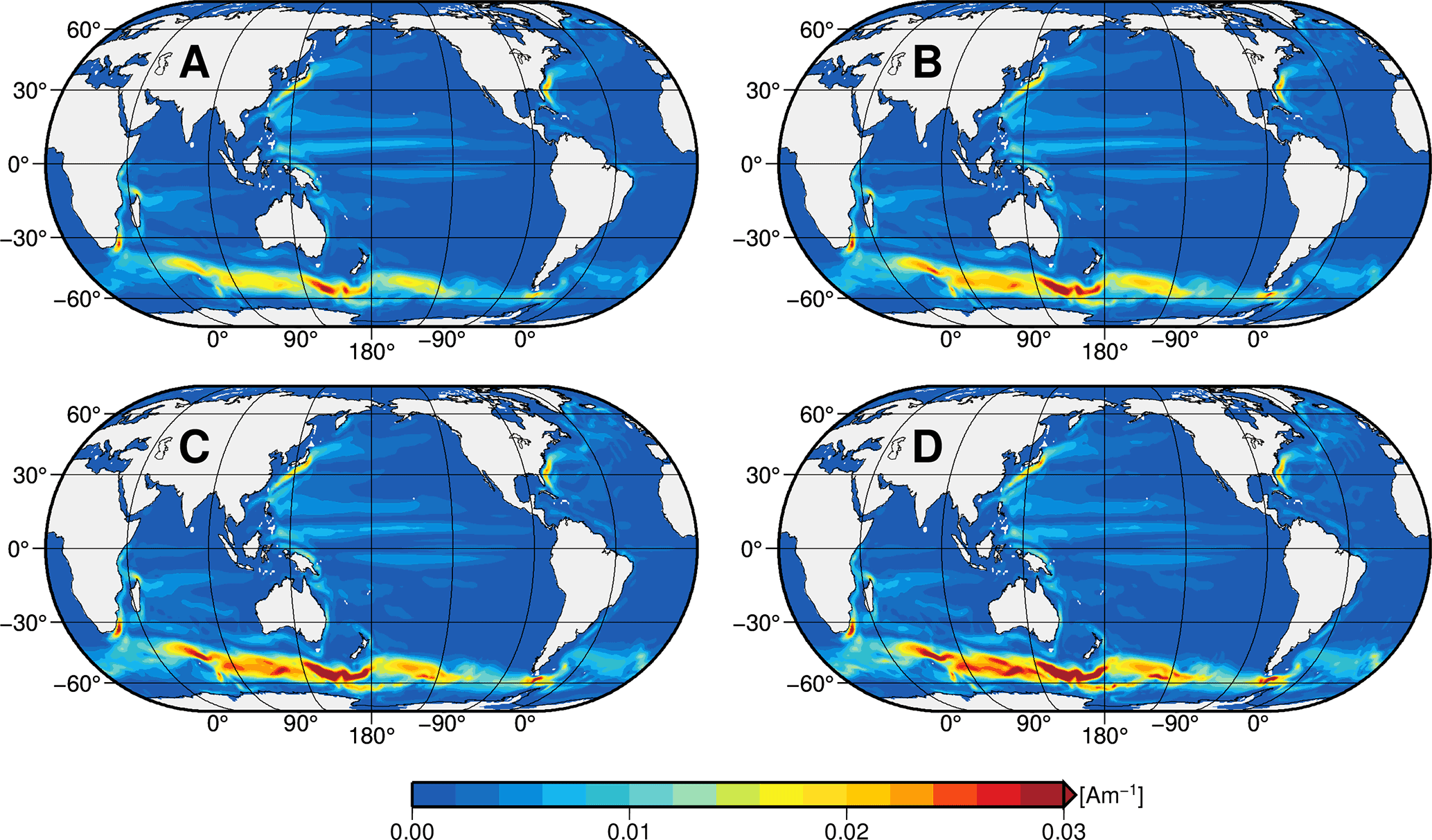
Figure 3Annual mean values of the upper layer oceanic electric current density jUp for scenarios A, B, C, and D with layer thicknesses of 1050, 1450, 2100, and 3000 m, respectively.
for . The resulting scenario-wise electric current densities in the upper layer, namely
are shown as annual mean values in Fig. 3. In each of the four scenarios it is assumed that the oceanic electric current density in the lower layer is equal to zero by setting ULo≡0. Thereby, the scenario-wise ocean-induced magnetic fields are solely generated by the ocean flow in the respective upper layer (see coloured layers in Fig. 2). The ocean conductance, in contrast, is identical to the reference simulation in all scenarios. Thus, the comparison between the scenario-wise ocean-induced magnetic fields and the reference ocean-induced magnetic field allows us to relate spatio-temporal patterns of the magnetic field to the generating ocean flow at different depths.
The consistency of this experiment setup was tested by subtracting the ocean-induced magnetic fields, which are generated by the upper and lower EM source layers, from the reference ocean-induced magnetic field. The differences between these fields, which arise due to EM coupling effects between the upper and lower source layers, are negligible compared to the magnetic signal strengths (not shown). Thereby, it is assured that the residual signals between the scenario-wise magnetic fields (considering only the upper EM source layers) and the reference magnetic field originate from the lower EM source layer.
3.1 Impact of sub-surface ocean flow on annual mean motional induction
The annual mean values of the scenario-wise ocean-induced magnetic fields at sea surface are shown in Fig. A1 of the Appendix. In all scenarios, strongest magnetic signals occur in the region of the Antarctic Circumpolar Current (ACC) with positive and negative values west and east of the southern geomagnetic equator, which is located between Australia and Antarctica. In contrast to the similar pattern, the scenario-wise increase in the upper EM source layer thickness has a considerable effect on the signal strength of the induced magnetic field. At sea surface, the mean ocean-induced magnetic field signal strength increases from scenario A (±2.5 nT) to D (±3.4 nT) as a result of the increasing electric current density (see Fig. 3). In addition, this increase is spatially non-uniform.
The annual mean residuals between the scenario-wise ocean-induced magnetic fields and the reference magnetic field (right plot in Fig. 1) are shown in Fig. 4. As the relevant residuals are located in the region of the ACC, only the Southern Hemisphere is depicted in Fig. 4. Due to the experiment setup, the residuals of the ocean-induced magnetic fields in each scenario originate from neglecting EM induction below the respective upper EM source layer. Thereby, the increase in the upper-layer thickness results in a general decrease in induced magnetic field residuals.
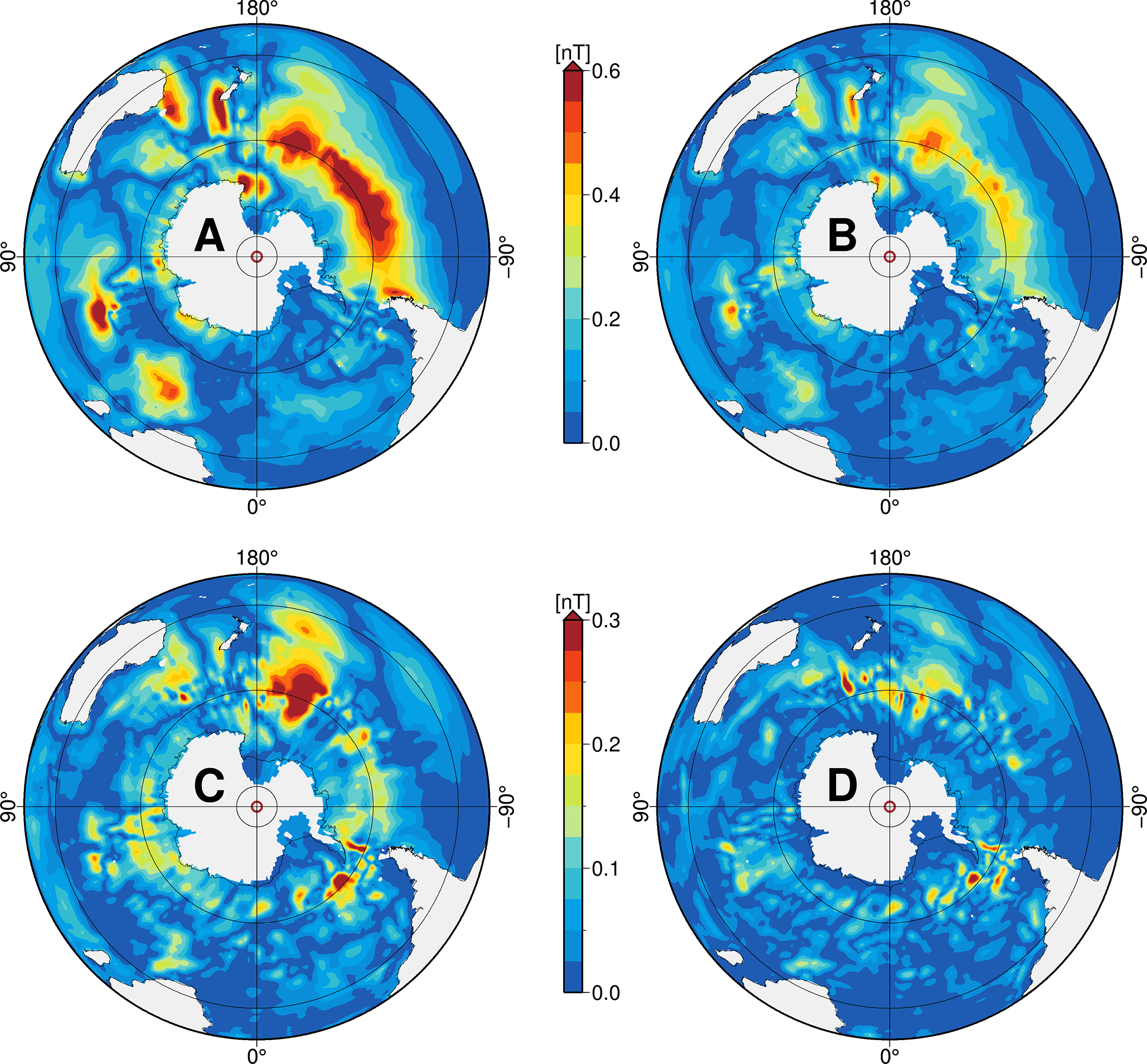
Figure 4Absolute values of annual mean ocean-induced magnetic field residuals at sea surface in the Southern Hemisphere for scenarios A, B, C, and D with layer thicknesses of 1050, 1450, 2100, and 3000 m, respectively. Note the different colour scale for scenarios C and D.
In scenario A (1050 m upper layer thickness), large-scale residuals occur in the southern Pacific Ocean around 60∘ S with values up to 0.7 nT (upper right quadrant in top left panel of Fig. 4). Largest residuals are found in small areas southwest of New Zealand (up to 0.8 nT) and in the southern Indian Ocean (up to 0.9 nT, lower left quadrant in top left panel). These residuals largely originate from the strong and deep-reaching eastward ocean currents in the ACC. In contrast to other major current systems, no lateral boundaries restrict the nearly zonal ocean flow around Antarctica. In this unique setting, zonal surface wind stress in the ACC region is balanced by ocean bottom form stress which, in turn, is maintained by strong top-to-bottom ocean flow (e.g. Munk and Palmén, 1951; Rintoul et al., 2001). Yet, very small residuals below 0.2 nT are found east of the Drake Passage (lower right quadrant of top left panel), which connects the tip of South America and the Antarctic Peninsula, although large mean transports of more than 170 Sv (1 Sv =106 m3s−1) can occur in this area (Donohue et al., 2016). In this region, however, the ACC flow is almost perpendicular to the gradient of the geomagnetic core field (not shown), resulting in weak oceanic electric currents and induced magnetic signals, regardless of the considered scenario (compare all panels in Fig. 4).
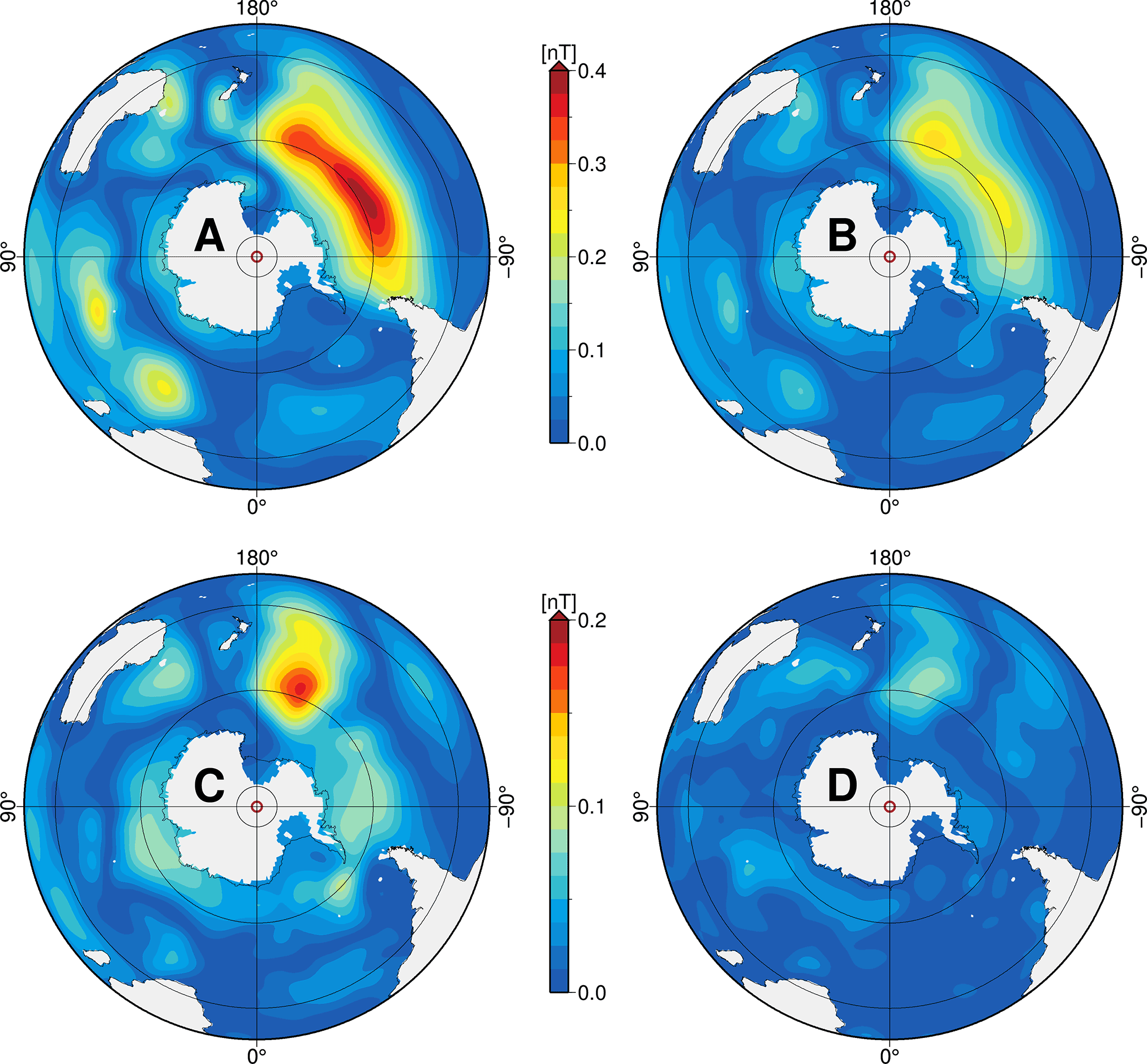
Figure 5Absolute values of annual mean ocean-induced magnetic field residuals at satellite altitude (430 km) in the southern hemisphere for scenarios A, B, C, and D with layer thicknesses of 1050, 1450, 2100, and 3000 m, respectively. Note the different colour scale for scenarios C and D.
In scenario B (1450 m upper layer thickness), the induced magnetic field residuals show a very similar spatial distribution as in scenario A. The upper layer thickness is increased by 400 m and, thus, the residuals compared to the reference simulation are generally smaller. Still, large-scale residuals amount to values between 0.4 and 0.5 nT, especially in the south Pacific Ocean (upper right quadrant of top right panel in Fig. 4).
In scenario C (2100 m upper layer thickness), the spatial distribution and magnitude of the induced magnetic field residuals change considerably. Note the smaller colour scale in scenarios C and D. In most regions, the values diminish below 0.2 nT. In addition, the distinctive residual pattern around 60∘ S in the South Pacific Ocean disintegrates in scenario C. Consequently, it can be concluded that in many regions in the Southern Hemisphere – e.g. southeast Pacific Ocean, south Indian Ocean, and south Atlantic Ocean – the strongest signals of the ocean-induced magnetic field are predominantly generated by strong ocean flow in the upper 2000 m of the ocean basin. The most prominent exception is located southeast of New Zealand, where the residuals still amount to 0.4 nT (upper right quadrant of bottom left panel in Fig. 4).
In scenario D (3000 m upper layer thickness), all large-scale residuals of the ocean-induced magnetic field vanish, leaving only local and weak residuals with values between 0.1 and 0.2 nT. These are located south and southeast of New Zealand and east of the Drake Passage (bottom right panel in Fig. 4).
The results of the four scenarios A to D show that deep and slow-moving ocean currents below 3000 m only have a marginal contribution to the strength of the ocean-induced magnetic field. Thereby, the strong wind-driven ocean currents in the upper ocean form the dominant EM source for the motional induction process, especially in the upper 2000 m of the ocean basin. Note that different results are to be expected for oceanic EM induction due to the M2 tide, which is often derived from barotropic tidal velocities (see, e.g., Schnepf et al., 2015; Grayver et al., 2016).
These findings can be directly transferred to the ocean-induced magnetic field at satellite altitude. For this, the scenario-wise ocean-induced magnetic field at 430 km above sea surface, and the corresponding magnetic field residuals compared to the reference simulation, are depicted in Figs. A2 and 5. Due to the upward continuation of the induced magnetic field to satellite altitude, small-scale patterns are blurred and weakened with increasing height (see also Vennerstrom et al., 2005; Manoj et al., 2006). The strongest remaining large-scale patterns are located in the region of the ACC with annual mean values between ±0.7 nT (A) and ±1.2 nT (D) (see Fig. A2). The resulting residuals between the scenario-wise ocean-induced magnetic fields and the reference show a similar, yet blurred, pattern distribution as it was visible at sea surface (compare Figs. 4 and 5). Corresponding to the strength of the induced magnetic signals, also the residuals' magnitude decreases with higher observation altitude. Hence, the largest residuals in scenario A reach values up to 0.4 nT in the South Pacific Ocean around 60∘ S, whereas residuals in scenario D remain below 0.1 nT (Fig. 5). The consequent implications for utilizing space-borne observations of motional induction are discussed in Sect. 3.3.

Figure 6(a) Power spectra of the annual mean ocean-induced magnetic fields at sea surface. (b) Absolute differences between the power spectra of the scenario-wise ocean-induced magnetic fields and the reference.
In addition to investigating the contribution of sub-surface ocean currents on motional induction by means of induced magnetic field residuals, we compare the spatial power spectra of the spherical harmonics based representation of the different oceanic magnetic fields (see details in Lowes, 1974) at sea surface height (Fig. 6). The restriction of the oceanic EM source to electric currents in the upper ocean results in a decrease in power in all degrees in the scenarios A to C (also for degrees higher than 15 not shown in Fig. 6). Thus, the dependence of motional induction on the EM source in the upper ocean is reflected by a shift of the power spectrum. Note, the similar power spectra offsets between scenarios A, B, C, and the reference result from very different upper layer thickness increments of 450, 650, and 3150 m, respectively (compare Figs. 2 and 6). The power spectra of scenario D and of the reference show a very close agreement. However, the power of degrees 3, 4, and 8 to 11 is visibly larger in scenario D than in the reference spectrum. This higher power is likely caused by neglecting deep ocean currents in the lower EM source layer in scenario D, which flow in the opposite direction compared to (near-)surface ocean currents. In the reference simulation, the electric current density in the ocean is considered in the form of a depth integral over the entire water column (see Eq. 2). Thus, opposing ocean currents can partially cancel each other out, which ultimately leads to the observed power reduction. One prominent example is the equator-ward flowing deep water in the Atlantic meridional overturning circulation that opposes the Gulf Stream (see, e.g., Srokosz and Bryden, 2015; Saynisch et al., 2016). Of course, scenarios A to C also neglect these deep water currents, but in these cases the effect of constraining the upper layer EM source results in much larger power spectra offsets. Here, again, it can be concluded that the inert water masses below 3000 m only have a small contribution to the signal strength of motional induction in the ocean, even though they can extent over more than 2000 m of the water column.
3.2 Impact of sub-surface ocean flow on annual variations of motional induction
The ocean-circulation-induced magnetic field contains a large static component due to the mean and quasi-steady large-scale ocean flow. This static component is hard to separate from other static magnetic field constituents – e.g. the crustal magnetic field (see also Kuvshinov, 2008). Hence, we also show the scenario-wise impact on the temporal variations of the circulation-induced magnetic field at the sea surface, which are depicted in Fig. A3.
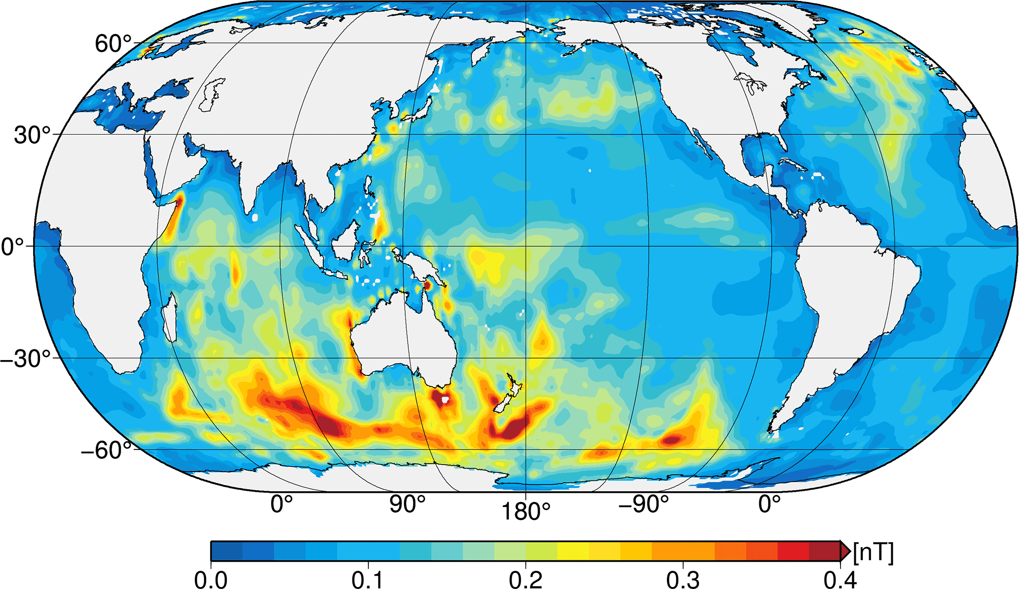
Figure 7Annual temporal variability (standard deviation) of the reference ocean-induced magnetic field.
The temporal variability of the reference oceanic magnetic field (Fig. 7) contains the known patterns and strength as they were previously calculated (see Manoj et al., 2006; Kuvshinov, 2008; Irrgang et al., 2016a). Strongest variability occurs in the region of the ACC, where also the strongest signals are located, with values up to 0.5 nT at the sea surface. The scenario-wise temporal variabilities reach larger magnitudes, especially in the ACC region southwest and southeast of Australia, with values up to 0.5 nT (A) and 0.7 nT (D) (Fig. A3). This amplification results from the exclusion of respective ocean currents in the lower EM source layer, which partially contain the same or similar temporal variability as ocean currents in the upper EM source layer. In other words, the barotropic ACC transport variability is constrained to the upper EM source layer (see also Cunningham, 2003). Thus, the strong baroclinic component of the temporal variability in the upper ocean has an enhanced effect of the motional induction process and is visible in the temporal variability of the scenario-wise motional induction. Interestingly, the scenario-wise temporal variabilities are not consistently decreasing with depth, as was shown for the scenario-wise mean magnetic field residuals in Sect. 3.1 (see Fig. 4). In particular, this is visible in the ACC region in the south Pacific Ocean between longitudes at 180 and −90∘ (compare reference and top left panel of Fig. A3). In this region, the temporal variability of the reference simulation is underrated by the corresponding values of scenario A. The temporal variations visible in the reference simulation first appear in scenario B, and are clearly distinct in scenarios C and D (Fig. A3). This is a first indication that observations of the ocean-induced magnetic field variability in this region could allow inferences on the ocean flow in the ACC below ocean depths of 1000 m, since the near-surface contribution in this region is small. Thereby, observed motional induction can not only lead to conclusions about the general ocean circulation in a depth-integrated sense, but also about transports and their spatio-temporal variability at specific depths in the ocean basin.
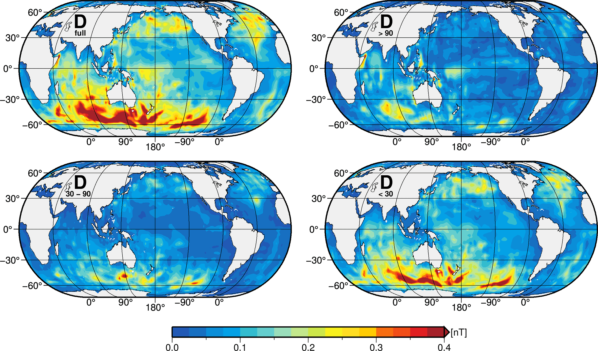
Figure 8Frequency analysis of the ocean-induced magnetic field variability (scenario D). Upper left: all periods. Upper right: seasonal periods longer than 90 days. Lower left: medium periods between 30 and 90 days. Lower right: short periods less than 30 days.
Using the example of scenario D, we performed a frequency analysis (Fourier transformation, Singleton, 1969) of the EM induction process during the 1-year simulation period. Figure 8 shows the temporal variability of the ocean-induced magnetic field in scenario D (upper left panel, same as in Fig. A3) and its corresponding decomposition into seasonal (more than 90 days, upper right panel), monthly (30 to 90 days, lower left panel), and sub-monthly (less than 30 days, lower right panel) time periods. The temporal transport variations in the ACC region are predominantly driven by fluctuations in the Southern Hemisphere wind regime (Bergmann and Dobslaw, 2012). Thus, the corresponding periods are transferred to the temporal variability of the ocean-induced magnetic signals and are visible in the respective frequency bands. The seasonal and monthly temporal variabilities show generally low values between 0.1 and 0.2 nT. Very local, monthly periods reach values of up to 0.3 nT south of Australia. The sub-monthly temporal variability reveals by far the highest values of up to 0.7 nT. The regional patterns in the ACC match closely the full temporal variability in scenario D (compare upper left and lower right panels in Fig. 8). Thus, strongest signals in the annual temporal variability of the ocean-induced magnetic field clearly coincide with signals due to the sub-monthly temporal variability of the ocean-induced magnetic field.
3.3 Implications for space-borne observations of motional induction
The space-borne observation of ocean-circulation-induced magnetic signals was defined as one of the objectives of ESA's satellite trio Swarm (Friis-Christensen et al., 2006). Assuming the nominal observation precision of 0.1 nT, Irrgang et al. (2017) demonstrated that artificial (i.e. model-based) satellite observations of the ocean-induced magnetic field can be used to correct water transports in a global ocean model with a data assimilation method. However, the signal separation of the ocean-circulation-induced magnetic signals is extremely challenging and has not been achieved to this day. This is not merely due to the nominal accuracy of satellite instruments, but largely due to the weak and irregular magnetic signals emitted by the ocean circulation. Furthermore, oceanic EM signals overlap in spatio-temporal extent with EM signals from other sources – e.g. from the ionosphere and from the Earth's crust and mantle (see, e.g., Kuvshinov, 2008). So far, these issues were only bypassed for tidally induced magnetic signals from the ocean (M2 and N2 constituents), where periods are known precisely and can be isolated from other EM sources (Sabaka et al., 2016). Nevertheless, the results presented here allow us to derive new insights on the information content of potential satellite observations of the ocean-circulation-induced magnetic field, which can help to improve future studies on motional induction due to the general ocean circulation.
The findings presented in Sect. 3.1 allow us to relate the ocean-induced magnetic field to the generating ocean currents at different depths (Figs. 4 and 5). In turn, ocean flow in specific regions and at specific depths can be corrected in future data assimilation studies, which might include actual Swarm satellite observations. In addition, it is shown in scenarios C and D that the magnetic field residuals at satellite altitude are weaker than the acknowledged threshold of 0.1 nT in many regions in the Southern Hemisphere. Consequently, even high-precision satellite observations of the ocean-induced magnetic field are likely insensitive to deep and inert ocean flow. Nevertheless, this observation technique includes valuable integrated information about oceanic transports, especially in the Antarctic Circumpolar Current, from the sea surface down to depths between 2000 and 3000 m. Moreover, if the correlations of ocean state variables (e.g. velocities, heat, and salinity) can be described accurately, these observations can also be used to improve model-based estimates about oceanic transports near the ocean bottom (Irrgang et al., 2017).
The results from Sect. 3.2 highlight that high-frequency variations of ocean currents on the sub-monthly timescale build a dominant forcing factor for the observable variability of motional induction in the ACC (particularly in the south Pacific Ocean). Thereby, space-borne observations of ocean magnetic anomalies with the respective signal strengths could be related to the generating sub-monthly ocean currents. Of course, these patterns can change when longer time spans are investigated. In particular, for decadal and longer periods, the influence of baroclinic processes in the ACC transport variability becomes increasingly important and can affect the found patterns (Olbers and Lettmann, 2007). Nevertheless, the frequency analysis over the period of one annual cycle provides an additional point of view on the information content of the ocean-induced magnetic field. In combination with the results shown in Sect. 3.1, it is evident that observations of the ocean-circulation-induced magnetic field contain more information about the ocean state than previously assumed. The prospect of utilizing these magnetic field measurements to infer properties about ocean currents at specific depths and time periods allows another step forward in observing ocean dynamics by its emitted magnetic signals.
The general ocean circulation model OMCT and the three-dimensional electromagnetic induction model X3DG are used to assess the sensitivity of oceanic motional induction towards ocean currents at different depths in the ocean basin. In a first-order approximation, the ocean-induced magnetic field is considered proportional to depth-integrated and conductivity-weighted ocean velocities. Consequently, oceanic electric currents are usually derived from these integrated quantities to build the source of electromagnetic induction in the ocean. However, the individual contribution of ocean currents at different depths towards the induction process has not yet been investigated.
In this study, we examine annual mean ocean-induced magnetic fields and their corresponding temporal variabilities, which are calculated in the frame of four different scenarios. In each of the four scenarios it is assumed that oceanic electric currents only occur between the sea surface and depth levels of 1050, 1450, 2100, and 3000 m, respectively. Oceanic electric currents below these upper layers are neglected in all scenarios. The resulting four scenario-wise ocean-induced magnetic fields are compared to a reference induced magnetic field, which is generated from electric currents over the entire water column.
The results of this study demonstrate that large-scale motional induction in the ocean is predominantly generated by wind-driven ocean currents in the upper ocean. Slow and inert ocean currents in the deeper ocean below 2000 m contribute only a small fraction to the annual mean magnetic field signal strength – even if these cover more than half of the water column. The largest residuals between the scenario-wise and the reference ocean-induced magnetic fields occur in the region of the deep-reaching Antarctic Circumpolar Current (ACC). Additionally, the spatial distribution of these residuals is very heterogeneous with largest patterns in the south Pacific Ocean. At the sea surface, the scenario-wise signal residuals reveal that ocean currents below 2000 m contribute up to 0.2 nT to the ocean-induced magnetic field signals strength in most regions. Locally, southeast of New Zealand, the residuals are larger with values of up to 0.4 nT. Ocean currents below 3000 m only add a marginal contribution to the ocean-induced magnetic field at the sea surface with regional and weak magnetic signatures between 0.1 and 0.2 nT. Similar, yet blurred and weakened, residuals between the scenario-wise and reference ocean-induced magnetic fields are identified at satellite altitude. Here, the annual mean magnetic signal contribution due to ocean currents below 3000 m remains under 0.1 nT. In addition to examining the scenario-wise annual mean ocean-induced magnetic fields strengths and residuals, their respective annual temporal variations are investigated. Our results indicate that observations of the oceanic magnetic signal variability could allow inferences on the generating sub-surface ocean currents below 1000 m. This relation seems particularly promising in the ACC region of the southeastern Pacific Ocean. Furthermore, the observed long-term temporal variability of motional induction could be related to intra-annual variabilities of ocean currents. More specifically, ocean currents with sub-monthly periods are found to dominate the annual temporal variability of the ocean-induced magnetic field.
The findings of this study have immediate implications for using potential space-borne observations of motional induction to infer properties about the general ocean circulation. The spatial relation between ocean-induced magnetic field signals and the generating ocean circulation can be used to localize the dominant EM current sources. Thereby, simulated oceanic transports in specific regions and at specific depths of the ocean basin can be examined, instead of assuming a worldwide uniform dependence of motional induction on ocean transports over the entire water column. Additionally, in the case that actual measurements of the annual temporal variability of motional induction in the ocean are separable from satellite observations, these could allow estimating the variability of oceanic transports within much shorter time periods. In combination, these features can support future studies on motional induction in the ocean, which aim to infer properties about large-scale ocean dynamics.
Researchers interested in using model data from the OMCT may contact Maik Thomas.
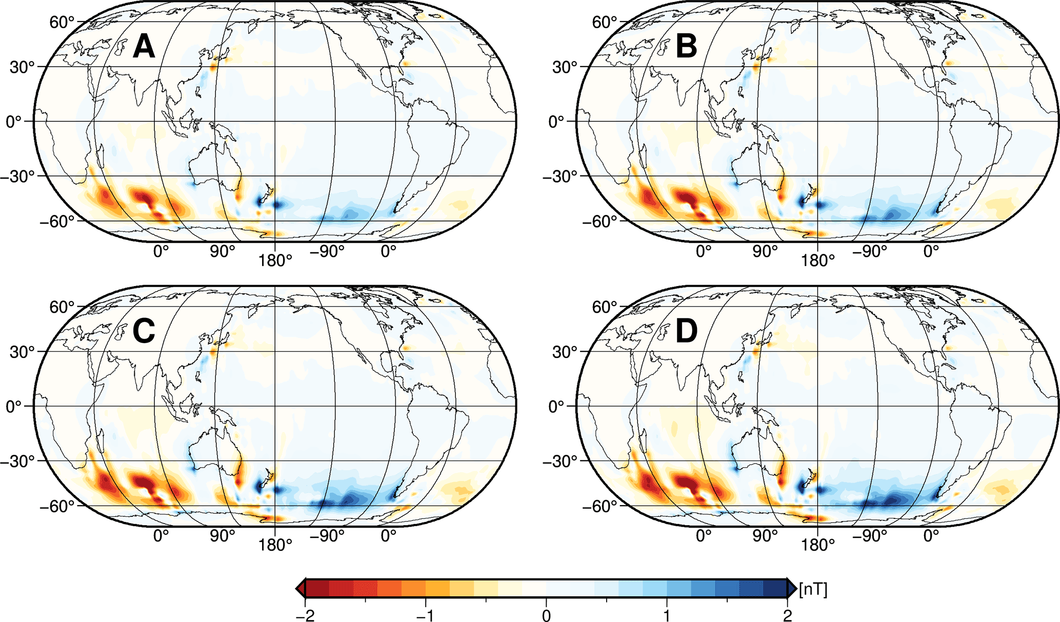
Figure A1Annual mean ocean-induced magnetic fields at sea surface for scenarios A, B, C, and D with layer thicknesses of 1050, 1450, 2100, and 3000 m, respectively.
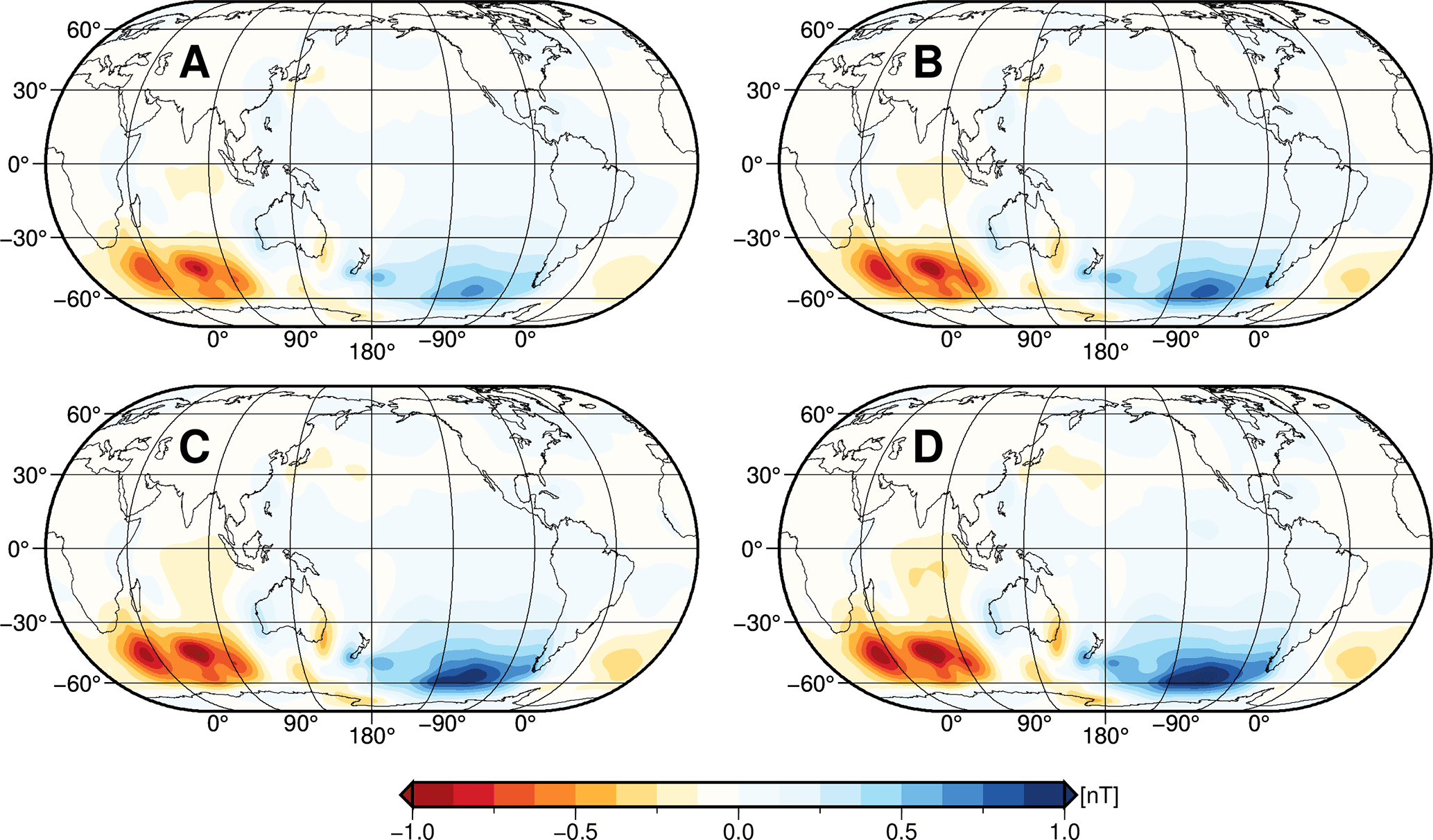
Figure A2Annual mean ocean-induced magnetic field at satellite altitude (430 km) for scenarios A, B, C, and D with layer thicknesses of 1050, 1450, 2100, and 3000 m, respectively.

Figure A3Annual temporal variability (standard deviation) of the ocean-induced magnetic field for scenarios A, B, C, and D with layer thicknesses of 1050, 1450, 2100, and 3000 m, respectively.
The authors declare that they have no conflict of interest.
This article is part of the special issue “Dynamics and interaction of processes in the Earth and its space environment: the perspective from low Earth orbiting satellites and beyond”. It is not associated with a conference.
We thank the editor, Jürgen Kusche, and the two anonymous reviewers for their
time and helpful remarks, which helped to improve this paper. This study
is funded by the German Research Foundation's priority programme 1788
“Dynamic Earth” and by the Helmholtz Association of German Research
Centres. We thank Alexey Kuvshinov for sharing his EM induction model, as
well as his expertise on the topic. We also thank the European Centre for
Medium-Range Weather Forecasts for providing the atmospheric reanalysis that
was used as forcing for the OMCT. Numerical simulations of the OMCT were
performed on the Mistral super computer from the German High Performance
Computing Centre for Climate and Earth System Research (DKRZ) in
Hamburg.
The article processing charges for this
open-access
publication were covered by a Research
Centre of the Helmholtz
Association.
The topical editor, Juergen Kusche, thanks two anonymous
referees for help in evaluating this paper.
Bergmann, I. and Dobslaw, H.: Short-term transport variability of the Antarctic Circumpolar Current from satellite gravity observations, J. Geophys. Res.-Oceans, 117, C05044, https://doi.org/10.1029/2012JC007872, 2012. a
Chave, A. D.: On the theory of electromagnetic induction in the Earth by ocean currents, J. Geophys. Res., 88, 3531–3542, https://doi.org/10.1029/JB088iB04p03531, 1983. a
Chave, A. D. and Luther, D. S.: Low-Frequency , Motionally Induced Electromagnetic Fields in the Ocean, 1. Theory, J. Geophys. Res., 95, 7185–7200, 1990. a
Cox, C. S.: On the electrical conductivity of the oceanic lithosphere, Phys. Earth Planet. In., 25, 196–201, https://doi.org/10.1016/0031-9201(81)90061-3, 1981. a
Cunningham, S. A.: Transport and variability of the Antarctic Circumpolar Current in Drake Passage, J. Geophys. Res., 108, 8084, https://doi.org/10.1029/2001JC001147, 2003. a
Dee, D. P., Uppala, S. M., Simmons, A. J., Berrisford, P., Poli, P., Kobayashi, S., Andrae, U., Balmaseda, M. a., Balsamo, G., Bauer, P., Bechtold, P., Beljaars, a. C. M., van de Berg, L., Bidlot, J., Bormann, N., Delsol, C., Dragani, R., Fuentes, M., Geer, a. J., Haimberger, L., Healy, S. B., Hersbach, H., Hólm, E. V., Isaksen, L., Kaallberg, P., Köhler, M., Matricardi, M., McNally, a. P., Monge-Sanz, B. M., Morcrette, J.-J., Park, B.-K., Peubey, C., de Rosnay, P., Tavolato, C., Thépaut, J.-N., and Vitart, F.: The ERA-Interim reanalysis: configuration and performance of the data assimilation system, Q. J. Roy. Meteor. Soc., 137, 553–597, https://doi.org/10.1002/qj.828, 2011. a
Dobslaw, H. and Thomas, M.: Simulation and observation of global ocean mass anomalies, J. Geophys. Res., 112, C05040, https://doi.org/10.1029/2006JC004035, 2007. a
Dobslaw, H., Flechtner, F., Bergmann-Wolf, I., Dahle, C., Dill, R., Esselborn, S., Sasgen, I., and Thomas, M.: Simulating high-frequency atmosphere-ocean mass variability for dealiasing of satellite gravity observations: AOD1B RL05, J. Geophys. Res., 118, 3704–3711, https://doi.org/10.1002/jgrc.20271, 2013. a, b
Donohue, K. A., Tracey, K. L., Watts, D. R., Chidichimo, M. P., and Chereskin, T. K.: Mean Antarctic Circumpolar Current transport measured in Drake Passage, Geophys. Res. Lett., 43, 11760–11767, https://doi.org/10.1002/2016GL070319, 2016. a
Everett, M. E., Constable, S., and Constable, C. G.: Effects of near-surface conductance on global satellite induction responses, Geophys. J. Int., 153, 277–286, https://doi.org/10.1046/j.1365-246X.2003.01906.x, 2003. a
Flosadóttir, A. H., Larsen, J. C., and Smith, J. T.: Motional induction in North Atlantic circulation models, J. Geophys. Res., 102, 10353–10372, https://doi.org/10.1029/96JC03603, 1997. a
Friis-Christensen, E., Lühr, H., and Hulot, G.: Swarm: A constellation to study the Earth's magnetic field, Earth Planets Space, 58, 351–358, https://doi.org/10.1186/BF03351933, 2006. a, b
Grayver, A. V., Schnepf, N. R., Kuvshinov, A. V., Sabaka, T. J., Manoj, C., and Olsen, N.: Satellite tidal magnetic signals constrain oceanic lithosphere-asthenosphere boundary., Sci. Adv., 2, e1600798, https://doi.org/10.1126/sciadv.1600798, 2016. a
Greatbatch, R. J.: A note on the representation of steric sea level in models that conserve volume rather than mass, J. Geophys. Res., 99, 12767, https://doi.org/10.1029/94JC00847, 1994. a
Irrgang, C., Saynisch, J., and Thomas, M.: Impact of variable seawater conductivity on motional induction simulated with an ocean general circulation model, Ocean Sci., 12, 129–136, https://doi.org/10.5194/os-12-129-2016, 2016a. a, b, c
Irrgang, C., Saynisch, J., and Thomas, M.: Ensemble simulations of the magnetic field induced by global ocean circulation: Estimating the uncertainty, J. Geophys. Res.-Oceans, 121, 1866–1880, https://doi.org/10.1002/2016JC011633, 2016b. a
Irrgang, C., Saynisch, J., and Thomas, M.: Utilizing oceanic electromagnetic induction to constrain an ocean general circulation model: A data assimilation twin experiment, J. Adv. Model. Earth Syst., 9, 1703–1720, https://doi.org/10.1002/2017MS000951, 2017. a, b, c, d
Kelbert, A., Kuvshinov, A., Velimsky, J., Koyama, T., Ribaudo, J., Sun, J., Martinec, Z., and Weiss, C. J.: Global 3-D electromagnetic forward modelling: a benchmark study, Geophys. J. Int., 197, 785–814, https://doi.org/10.1093/gji/ggu028, 2014. a
Kuvshinov, A.: 3-D Global Induction in the Oceans and Solid Earth: Recent Progress in Modeling Magnetic and Electric Fields from Sources of Magnetospheric, Ionospheric and Oceanic Origin, Surv. Geophys., 29, 139–186, https://doi.org/10.1007/s10712-008-9045-z, 2008. a, b, c, d, e
Kuvshinov, A. and Semenov, A.: Global 3-D imaging of mantle electrical conductivity based on inversion of observatory C-responses-I. An approach and its verification, Geophys. J. Int., 189, 1335–1352, https://doi.org/10.1111/j.1365-246X.2011.05349.x, 2012. a
Larsen, J. C.: Electric and Magnetic Fields Induced by Deep Sea Tides, Geophys. J. Roy. Astr. S., 16, 47–70, https://doi.org/10.1111/j.1365-246X.1968.tb07135.x, 1968. a
Laske, G. and Masters, G.: A global digital map of sediment thickness, Eos Trans. AGU, Fall Meet. Suppl., 78, F483, 1997. a
Lowes, F. J.: Spatial Power Spectrum of the Main Geomagnetic Field, and Extrapolation to the Core, Geophys. J. Int., 36, 717–730, https://doi.org/10.1111/j.1365-246X.1974.tb00622.x, 1974. a
Manoj, C., Kuvshinov, A., Maus, S., and Lühr, H.: Ocean circulation generated magnetic signals, Earth Planets Space, 58, 429–437, https://doi.org/10.1186/BF03351939, 2006. a, b, c
Minami, T.: Motional Induction by Tsunamis and Ocean Tides: 10 Years of Progress, Surv. Geophys., 38, 1097–1132, https://doi.org/10.1007/s10712-017-9417-3, 2017. a
Munk, W. H. and Palmén, E.: Note on the Dynamics of the Antarctic Circumpolar Current, Tellus, 3, 53–55, https://doi.org/10.3402/tellusa.v3i1.8609, 1951. a
Olbers, D. and Lettmann, K.: Barotropic and baroclinic processes in the transport variability of the Antarctic Circumpolar Current, Ocean Dynam., 57, 559–578, https://doi.org/10.1007/s10236-007-0126-1, 2007. a
Püthe, C., Kuvshinov, A., Khan, A., and Olsen, N.: A new model of Earth's radial conductivity structure derived from over 10 yr of satellite and observatory magnetic data, Geophys. J. Int., 203, 1864–1872, https://doi.org/10.1093/gji/ggv407, 2015. a
Rintoul, S., Hughes, C., and Olbers, D.: The antarctic circumpolar current system, in: International Geophysics, Elsevier, vol. 77, chap. 4.6, 271–302, https://doi.org/10.1016/S0074-6142(01)80124-8, 2001. a
Sabaka, T. J., Tyler, R. H., and Olsen, N.: Extracting Ocean-Generated Tidal Magnetic Signals from Swarm Data through Satellite Gradiometry, Geophys. Res. Lett., 43, 3237–3245, https://doi.org/10.1002/2016GL068180, 2016. a
Sanford, T. B.: Motionally induced electric and magnetic fields in the sea, J. Geophys. Res., 76, 3476–3492, https://doi.org/10.1029/JC076i015p03476, 1971. a
Saynisch, J., Bergmann-Wolf, I., and Thomas, M.: Assimilation of GRACE-derived oceanic mass distributions with a global ocean circulation model, J. Geodesy, 89, 121–139, https://doi.org/10.1007/s00190-014-0766-0, 2014. a
Saynisch, J., Petereit, J., Irrgang, C., Kuvshinov, A., and Thomas, M.: Impact of climate variability on the tidal oceanic magnetic signal-A model-based sensitivity study, J. Geophys. Res.-Oceans, 121, 5931–5941, https://doi.org/10.1002/2016JC012027, 2016. a, b
Schnepf, N. R., Kuvshinov, A., and Sabaka, T.: Can we probe the conductivity of the lithosphere and upper mantle using satellite tidal magnetic signals?, Geophys. Res. Lett., https://doi.org/10.1002/2015GL063540, 2015. a
Singleton, R.: An algorithm for computing the mixed radix fast Fourier transform, IEEE T. Acoust. Speech, 17, 93–103, https://doi.org/10.1109/TAU.1969.1162042, 1969. a
Srokosz, M. A. and Bryden, H. L.: Observing the Atlantic Meridional Overturning Circulation yields a decade of inevitable surprises, Science, 348, 1255575–1–1255575–5, https://doi.org/10.1126/science.1255575, 2015. a
Stephenson, D. and Bryan, K.: Large-scale electric and magnetic fields generated by the oceans, J. Geophys. Res., 97, 15467–15480, https://doi.org/10.1029/92JC01400, 1992. a, b
Thébault, E., Finlay, C. C., Beggan, C. D., Alken, P., Aubert, J., Barrois, O., Bertrand, F., Bondar, T., Boness, A., Brocco, L., Canet, E., Chambodut, A., Chulliat, A., Coïsson, P., Civet, F., Du, A., Fournier, A., Fratter, I., Gillet, N., Hamilton, B., Hamoudi, M., Hulot, G., Jager, T., Korte, M., Kuang, W., Lalanne, X., Langlais, B., Léger, J.-M., Lesur, V., Lowes, F. J., Macmillan, S., Mandea, M., Manoj, C., Maus, S., Olsen, N., Petrov, V., Ridley, V., Rother, M., Sabaka, T. J., Saturnino, D., Schachtschneider, R., Sirol, O., Tangborn, A., Thomson, A., Tøffner-Clausen, L., Vigneron, P., Wardinski, I., and Zvereva, T.: International Geomagnetic Reference Field: the 12th generation, Earth Planets Space, 67, 79, https://doi.org/10.1186/s40623-015-0228-9, 2015. a
Thomas, M., Sündermann, J., and Maier-Reimer, E.: Consideration of ocean tides in an OGCM and impacts on subseasonal to decadal polar motion excitation, Geophys. Res. Lett., 28, 2457–2460, https://doi.org/10.1029/2000GL012234, 2001. a
Tyler, R. H., Mysak, L. A., and Oberhuber, J. M.: Electromagnetic fields generated by a three dimensional global ocean circulation, J. Geophys. Res., 102, 5531–5551, https://doi.org/10.1029/96JC03545, 1997. a, b
Vennerstrom, S., Friis-Christensen, E., Lühr, H., Moretto, T., Olsen, N., Manoj, C., Ritter, P., Rastätter, L., Kuvshinov, A., and Maus, S.: The Impact of Combined Magnetic and Electric Field Analysis and of Ocean Circulation Effects on Swarm Mission Performance, Tech. rep., Danish National Space Center, Kgs. Lyngby, Denmark, 2005. a
Vivier, F., Meier-Reimer, E., and Tyler, R. H.: Simulations of magnetic fields generated by the Antarctic Circumpolar Current at satellite altitude: Can geomagnetic measurements be used to monitor the flow?, Geophys. Res. Lett., 31, L10306, https://doi.org/10.1029/2004GL019804, 2004. a, b