The asymmetric geospace as displayed during the geomagnetic storm on 17 August 2001

Previous studies have shown that conjugate auroral features are displaced in the two hemispheres when the interplanetary magnetic field (IMF) has a transverse (Y) component. It has also been shown that a B_Y component is induced in the closed magnetosphere due to the asymmetric loading of magnetic flux in the lobes following asymmetric dayside reconnection when the IMF has a Y component. The magnetic field lines with azimuthally displaced footpoints map into a “banana”-shaped convection cell in one hemisphere and an “orange”-shaped cell in the other. Due to the Parker spiral our system is most often exposed to a B_Y-dominated IMF. The dipole tilt angle, varying between $\pm \mathrm{34}{}^{\circ }$, leads to warping of the plasma sheet and oppositely directed B_Y components in dawn and dusk in the closed magnetosphere. As a result of the Parker spiral and dipole tilt, geospace is asymmetric most of the time. The magnetic storm on 17 August 2001 offers a unique opportunity to study the dynamics of the asymmetric geospace. IMF B_Y was 20–30 nT and tilt angle was 23^∘. Auroral imaging revealed conjugate features displaced by 3–4 h magnetic local time. The latitudinal width of the dawnside aurora was quite different (up to 6^∘) in the two hemispheres. The auroral observations together with convection patterns derived entirely from measurements indicate dayside, lobe and tail reconnection in the north, but most likely only dayside and tail reconnection in the Southern Hemisphere. Increased tail reconnection during the substorm expansion phase reduces the asymmetry.

1 Introduction

Over the last 2 decades it has been well established that the transverse component, B_Y, of the interplanetary magnetic field (IMF) leads to longitudinal displacement of the aurora in the conjugate hemispheres (Liou and Newell, 2010; Liou et al., 2001b; Wang et al., 2007; Østgaard et al., 2004, 2005, 2011b). As similar auroral features in the two hemispheres can be considered as an illuminated footprint of conjugate magnetic field lines, these findings provide evidence of an “added” B_Y component in the closed magnetosphere with the same polarity as the IMF B_Y. This adds to the well known convection pattern asymmetry, with “orange” and “banana” cells due to IMF B_Y (Heppner and Maynard, 1987), which are approximately mirrored in the two hemispheres. However, the question of how a B_Y component is established in the closed magnetosphere has been controversial. It has often been referred to as a simple “penetration” of IMF B_Y (Kozlovsky et al., 2003; Petrukovich, 2011; Rong et al., 2015), while others have suggested that B_Y is transported into the closed magnetosphere through tail reconnection (Motoba et al., 2010; Stenbaek-Nielsen and Otto, 1997; Østgaard et al., 2004). In this study we will show that increased tail reconnection has rather the opposite effect: it reduces asymmetry. In a recent paper Tenfjord et al. (2015) developed a more comprehensive understanding of how a B_Y component is established in the closed magnetosphere. Adapting the ideas first suggested by Cowley (1981), but further developed to be consistent with observations by Khurana et al. (1996), Tenfjord et al. (2015) argued that it is the asymmetric loading of magnetic flux in the lobes following dayside reconnection that induces a B_Y component in the closed magnetosphere. It is the magnetic pressure force from the lobes that affects the closed magnetosphere, and the term “penetration” of fields is misleading. Tenfjord et al. (2015) used magnetohydrodynamics (MHD) modeling to predict that the B_Y component would be induced after just a few minutes. Tenfjord et al. (2015) also laid out a dynamical scenario of how the induced B_Y component would lead to an asymmetric launch of Alfvénic waves and currents into the hemisphere where the field line is connected to the “banana” cell. The ionospheric convection speed on the equatorward part of the “banana” cell was also predicted to be faster in order to restore symmetry closer to Earth. This was later confirmed by Reistad et al. (2016). In two follow-up papers Tenfjord et al. (2017, 2018), based on observational data from geosynchronous orbit (see also Wing et al., 1995), showed that B_Y was indeed induced on the closed field lines after only 5 to 10 min, similar to the response time between IMF orientation change and ionospheric convection change reported by Ridley et al. (1998) and Snekvik et al. (2017). These results (Tenfjord et al., 2017, 2018) support the modeling results from Tenfjord et al. (2015) and contradict the claims that reconnection is the mechanism by which a B_Y component is transported into the closed magnetosphere. The latter would require about 1–2 h response time (Browett et al., 2017; Motoba et al., 2010; Rong et al., 2015) corresponding to the convection time from dayside to nightside across the polar cap. In the present study we will show that the role of increased tail reconnection is quite different. The importance of these studies are underpinned by the following: as the IMF orientation is distributed as a Parker spiral, it can be shown that the strictly northward- or southward-dominated orientation, often studied, is a rather rare situation, while a B_Y-dominated IMF ($\left|B_Y\right|>\left|B_Z\right|$) is the common orientation (>70 % of the time). This means that most of the time we have asymmetric loading of magnetic flux, asymmetric footpoints of magnetic field lines, asymmetric aurora, currents and convection pattern. To put it briefly: geospace is most often asymmetric. To understand why and when, and how large the asymmetries are, is crucial for all studies involving mapping as well as any prediction efforts. During IMF B_Y-dominated conditions, the dayside, lobe and tail reconnections are expected to occur simultaneously (Nishida et al., 1998; Reiff and Burch, 1985; Sandholt et al., 1998), but the occurrence of lobe reconnection may also depend on the tilt angle (Crooker and Rich, 1993). The dipole tilt also leads to warping of the plasma sheet in the magnetotail (Tsyganenko, 1998) and induces oppositely directed B_Y components in the closed magnetosphere at dusk and dawn. As the dipole tilt angle is varying between $\pm \mathrm{34}{}^{\circ }$ this is also a factor creating an asymmetric geospace.

The magnetic storm on 17 August 2001 offers a unique opportunity to study how all these effects are dynamically interrelated when we have a large IMF B_Y component (>20 nT), large tilt angle (23^∘) and two substorms with increased tail reconnection in their expansion phase. This magnetic storm was also studied by Longley et al. (2017b) who used conjugate auroral imaging to determine the dawn–dusk offset of the polar cap between the hemispheres and compared those with four different MHD model predictions. They found that none of the models reproduced the observed polar cap width. They also suggested that lobe reconnection was present in the Northern Hemisphere. In a follow up paper Longley et al. (2017a) also addressed the polar cap width, but focused more on the auroral data. They repeated the claim about seeing signatures of lobe reconnection in a Defense Meteorological Satellite Program (DMSP) pass in the Northern Hemisphere.

In the present paper we will use the same imaging data to identify discrete conjugate auroral features as well as sudden simultaneous brightening in order to study the asymmetric geospace during this magnetic storm. When using the term “discrete” we refer to distinct features produced by accelerated electrons that are sufficiently bright to be identified. They may be discrete arcs, but the spatial resolution of the cameras does not allow us to determine that unambiguously. This identification and the analysis we perform are based on the following assumptions:

• a.

  As they are known to be associated with field-aligned currents, discrete auroral features produced by acceleration and subsequent electron precipitation are a manifestation of coupling between the magnetosphere and ionosphere (Ohtani et al., 2009). When identifying discrete auroral features in the conjugate hemispheres, we will look for similar shapes – not necessarily identical, but sufficiently bright to be identified. We emphasize that we do not intend to compare absolute auroral intensities, which could be affected by both different conductivity and different acceleration along field lines.

• b.

  When auroral features with similar shapes and/or similar dynamical behavior can be identified simultaneously in both hemispheres, it is a strong indication that these features have a common magnetospheric source region. As will be shown, we identify relatively bright poleward features indicative of tail reconnection, which by definition are magnetically connected. Although it is an open question as to how the electrons are accelerated to produce poleward boundary intensifications (Ohtani and Yoshikawa, 2016; Øieroset et al., 2002), there is observational evidence that bright auroral features at the nightside poleward boundary are found at the footpoint of reconnected field lines in the tail (Borg et al., 2007; Østgaard et al., 2009). We also identify features that brighten up simultaneously in both hemispheres (a dynamical change, similar to substorm onset), which is also a strong indicator of having a common magnetospheric source and being magnetically connected.

With 2 h of simultaneous conjugate auroral imaging we observed conjugate auroral features displaced by 3–4 h MLT, similar to the 3 h MLT reported by Reistad et al. (2016). The latitudinal width of the dawnside aurora was much larger in the Northern than the Southern Hemisphere. Convection patterns derived from measurements only, combined with the auroral features indicate dayside, lobe and tail reconnection in the Northern Hemisphere, but only dayside and tail reconnection in the Southern Hemisphere. As two substorms occurred during this 2 h period, we find that increased tail reconnection does not transport B_Y components into the closed magnetosphere, but rather reduces the asymmetry by partly removing the magnetic pressure in the lobes. A similar reduction of asymmetry during the substorm expansion phase was reported by Østgaard et al. (2011a). Reduction of the B_Y-dependent dawn–dusk asymmetry in convection pattern after substorm onset has also been reported by Grocott et al. (2010).

After presenting our analysis of these asymmetric auroral features, we will discuss the implications of considering these features as not being conjugate, that they may result from either ionospheric processes, conductivity differences or have different sources in the magnetosphere.

2 Data

During the magnetic storm on 17 August 2001 the IMAGE and Polar Mission spacecraft provided 5 h of imaging data from the same (northern) hemisphere and later more than 2 h of simultaneous images from the conjugate hemispheres. The IMAGE Far UltraViolet instrument package provided images in three different wavelength bands (Mende et al., 2000): IMAGE-WIC, 140–180 nm, which includes the Lyman–Birge–Hopfield (LBH) N₂ band and a few nitrogen lines; IMAGE-SI12, Doppler-shifted Lyman α (121.8 nm); and IMAGE-SI13, oxygen emission (135.6 nm). The Polar VIS Earth camera (Frank et al., 1995) measured emissions in the 124–149 nm band, which is usually dominated by the atomic oxygen (OI) line at 130.4 nm but with contributions from oxygen line at 135.6 nm, the LBH N₂ band and a nitrogen line (Frank and Sigwarth, 2003), dependent on the electron energies (Frey et al., 2003a). To identify similar auroral features we have used IMAGE SI13 and Polar VIS, and in Sect. 3 we discuss the importance of comparing images from cameras that are as identical as possible. Exposure times are 5, 10 and 32.5 s and cadences are 123, 123 and 54 s for IMAGE SI13, IMAGE WIC and Polar VIS Earth camera, respectively. For all the imaging data presented in this paper APEX coordinates are used.

The solar wind and IMF measurements are provided by ACE through the OMNI data (King and Papitashvili, 2005). They are time-shifted to the subsolar bow shock location.

To establish a convection pattern we use data from SuperDARN (Greenwald et al., 1995), SuperMAG (Gjerloev, 2012) and DMSP (Rich and Hairston, 1994). How the convection patterns are calculated will be explained in Sect. 3. CHAMP (Reigber et al., 2002) data are used to derive field-aligned currents (Lühr et al., 1996). For SuperMAG and DMSP we have used APEX coordinates, while for SuperDARN AACGM coordinates are used. The APEX and AACGM coordinate systems are almost identical (Laundal and Richmond, 2016) at high latitudes and the difference is negligible for the results presented in this paper.

There are large amounts of data that have been considered for the analysis presented in this paper. For transparency, we have uploaded a video (Supplement) showing the data coverage for the time interval from 15:50 to 18:59 UT. This comprises three channels of IMAGE data (SI12, SI13 and WIC), the Polar VIS images, SuperDARN line-of-sight coverage (green dots) and vectors from overlapping radars (green vectors), SuperMAG magnetic field perturbations rotated in the direction of an equivalent overhead current (brown vectors), DMSP and NOAA electron energy flux (pink bars), DMSP ion flow (green lines) and field-aligned currents derived from CHAMP data (red: upward current; blue: downward current). In this paper we will present a selection of the most prominent features in the imaging data as well as particle data and modeling results to support our interpretation.

3 Methodology

Simultaneous images from the conjugate hemispheres are used to identify asymmetric auroral features. The IMAGE far ultraviolet (FUV) images were pre-processed using the FUVIEW3 software (http://sprg.ssl.berkeley.ed/image/, last access: 5 July 2012) with the “corrected counts” option, ensuring that intensity across the detector (flat-field correction) and from different times of the mission (temperature correction) can be compared. For the SI13 camera we used an updated flat field as the default flat field did not perform well on the dayside during this event. The VIS Earth image data were downloaded from NASA's Space Physics Data Facility (ftp://cdaweb.gsfc.nasa.gov/pub/data/polar/vis/vis_earth-camera-full/, last access: 5 July 2012) and processed using the XVIS 2.40 software (http://vis.physics.uiowa.edu/vis/software/, last access: 5 July 2012), which includes a flat-field correction and the most updated values for pointing information.

The dayglow-induced emissions and background noise have been subtracted from each image separately. This is done by constructing a model of the dayglow emissions from pixels not influenced by aurora based on their solar zenith angle and satellite zenith angle in the mapped image. The modeled pixel intensity is then subtracted from all pixels, leaving only auroral emissions in the image. The Poisson variation of the dayglow will still remain as noise in the image (Reistad et al., 2014).

Ideally, we would use images from identical calibrated cameras for this, but unfortunately such auroral cameras in space do not exist. The best we can do is to use cameras that at least detect emissions from the same constituents of the atmosphere. As VIS Earth and SI13 cameras are both predominantly detecting emissions from atomic oxygen, we assume that intensity changes due to varying relative densities of nitrogen versus oxygen should be small. However, they are detecting different emission lines, namely 130.4 nm (VIS) and 135.6 nm (SI13), have different contributions from the LBH band and different scattering cross sections, so we need to perform an intercalibration as best we can. For this we use the 5 h of data gathered when the two cameras were imaging the same aurora from the Northern Hemisphere and scale the intensities to display similar features. An example is shown in Fig. 1. Although the VIS image has different pixel resolution than SI13 (256×256 versus 128×128), the two images (Fig. 1a and b) display similar auroral features with approximately the same intensities. The scaling between SI13 and VIS is not only based on this pair of images, but all the images when the two cameras were detecting the same aurora in the Northern Hemisphere (10:00–15:00 UT). The purpose is to establish a scaling that will be used for comparing SI13 and VIS when they observed the aurora simultaneously in the Northern and Southern Hemisphere, respectively.

We also show the IMAGE WIC image, with two different color scalings, just to illustrate how differently the same auroral oval appears in a different wavelength band. If the two images from IMAGE-WIC and Polar VIS (Fig. 1c and b), where the aurora in the dawn is scaled to match, had been from the conjugate hemispheres we would probably conclude that the dusk side aurora are fairly asymmetric in intensity. However, it is more likely that the dusk side aurora should be scaled to match (Fig. 1b and d) and that it is indeed the dawnside aurora that appears with much higher intensities in the WIC image than in the VIS image. Such a difference could then be explained by more energetic electrons drifting towards dawn where they are scattered into the loss cone by waves and precipitate, which will appear more intense in the LBH band than in the 130.4 nm emissions (Frey et al., 2003a), as Fig. 1d clearly shows when compared to Fig. 1b. As WIC (LBH) and VIS (130.4 nm) respond differently to energetic precipitation, we will only use data from SI13 and VIS (with the scaling established in Fig. 1) to identify conjugate auroral features. There are also other technical issues that can lead to misinterpretation of auroral features and those are different viewing angles and dayglow subtraction. Auroral intensities obtained from very oblique viewing angles would be different than from nadir depending on the auroral structures, so care should be taken when looking at features that are imaged from slant angles. The dayglow removal can also introduce features or remove features. In our dayglow removal we make sure that what is left of counts equatorward of the dayside oval has a mean value of zero when averaged over a sufficiently large area. Conductivity differences could also lead to misinterpretation as they are known to give different auroral intensities (Liou et al., 2001a; Newell et al., 1996). However, we emphasize that we do not intend to compare absolute intensities, only discrete auroral features sufficiently bright to be identified.

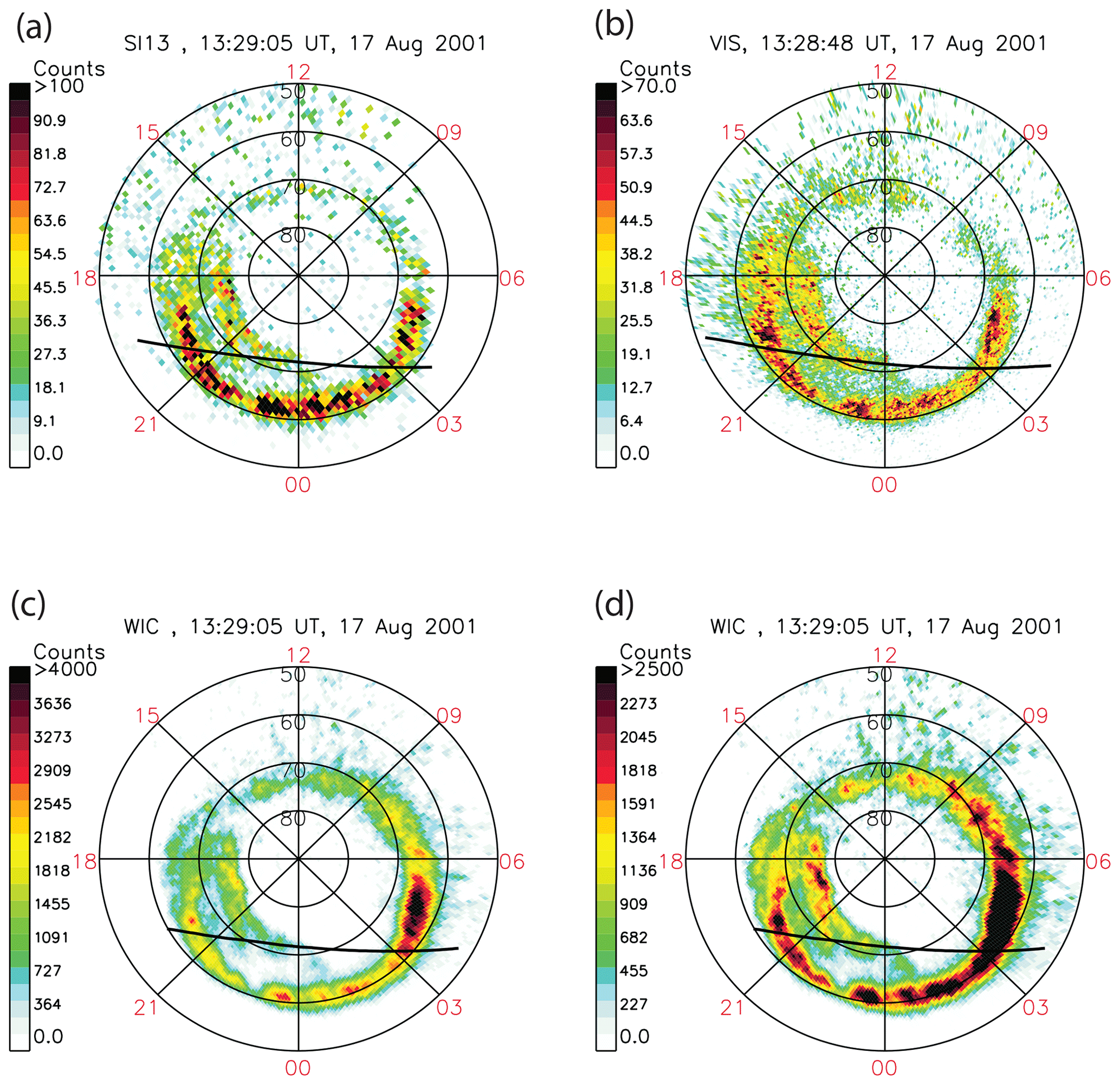
Figure 1 Images of different emission bands at 13:29 UT, 17 August 2001, separated by ∼15 s (center time). All images are from the Northern Hemisphere. Black lines indicate the terminator at 90^∘ solar zenith angle. (a) IMAGE SI13; (b) Polar VIS; (c) IMAGE WIC, where the dawn aurora is scaled to match VIS; (d) IMAGE WIC, where the dusk aurora is scaled to match VIS.

To estimate the global plasma flow pattern (in a corotating frame), we adopt a novel purely data-based multi-instrument approach, without using any empirical model to fill in regions with data gaps. If the plasma is incompressible, i.e., if $\mathrm{\nabla }\cdot v=\mathrm{0}$, v can be expressed in terms of spherical elementary convection cells, similar to the much used spherical elementary current cell technique developed by Amm (1997). This was demonstrated in a local region, using SuperDARN measurements, by Amm et al. (2010). Here we use a global (poleward of 50^∘) grid of elementary convection cells, and estimate their amplitudes through a set of linear equations (Amm et al., 2010). As input we use three different datasets: (1) SuperDARN line-of-sight measurements of the plasma flow, providing one equation per measurement; (2) DMSP SSIES measurements of the vector flow, adding two equations per measurement (we use only measurements obtained within ±2 min of the time of the convection map); and (3) measurements from SuperMAG, of the ground magnetic field, assuming that they correspond to currents opposite of the flow (Hall currents), and that 1 nT corresponds to 2 m s⁻¹. Laundal et al. (2015, 2016) showed that the assumption that the average equivalent current is the Hall current, and therefore can be used to find convection direction, is reasonable in sunlight (but only then). However, the conversion from 1 nT to 2 m s⁻¹ is questionable, so we weight the equations associated with these measurements by 0.3. That means that they only become important in regions where no actual flow measurements are available. In addition to the measurements, we pad the circle at 50^∘ with measurements of zero flow relative to a corotating frame, as a weakly imposed boundary condition.

The underdetermined set of equations is solved by singular value decomposition, zeroing singular values that are smaller than 5 % of the largest value. We present the result in terms of the flow stream function ψ, which relates to the velocity by

$$\begin{array}{}\text{(1)}& v=\widehat{\mathit{r}}\times \mathrm{\nabla }\mathit{\psi },\end{array}$$

where $\widehat{\mathit{r}}$ is a unit vector in the radial direction. Note that ψ is not the same as the electric potential, yet they are similar.

4 The magnetic storm on 17 August 2001

We will now present the data obtained during the magnetic storm 17 August 2001.

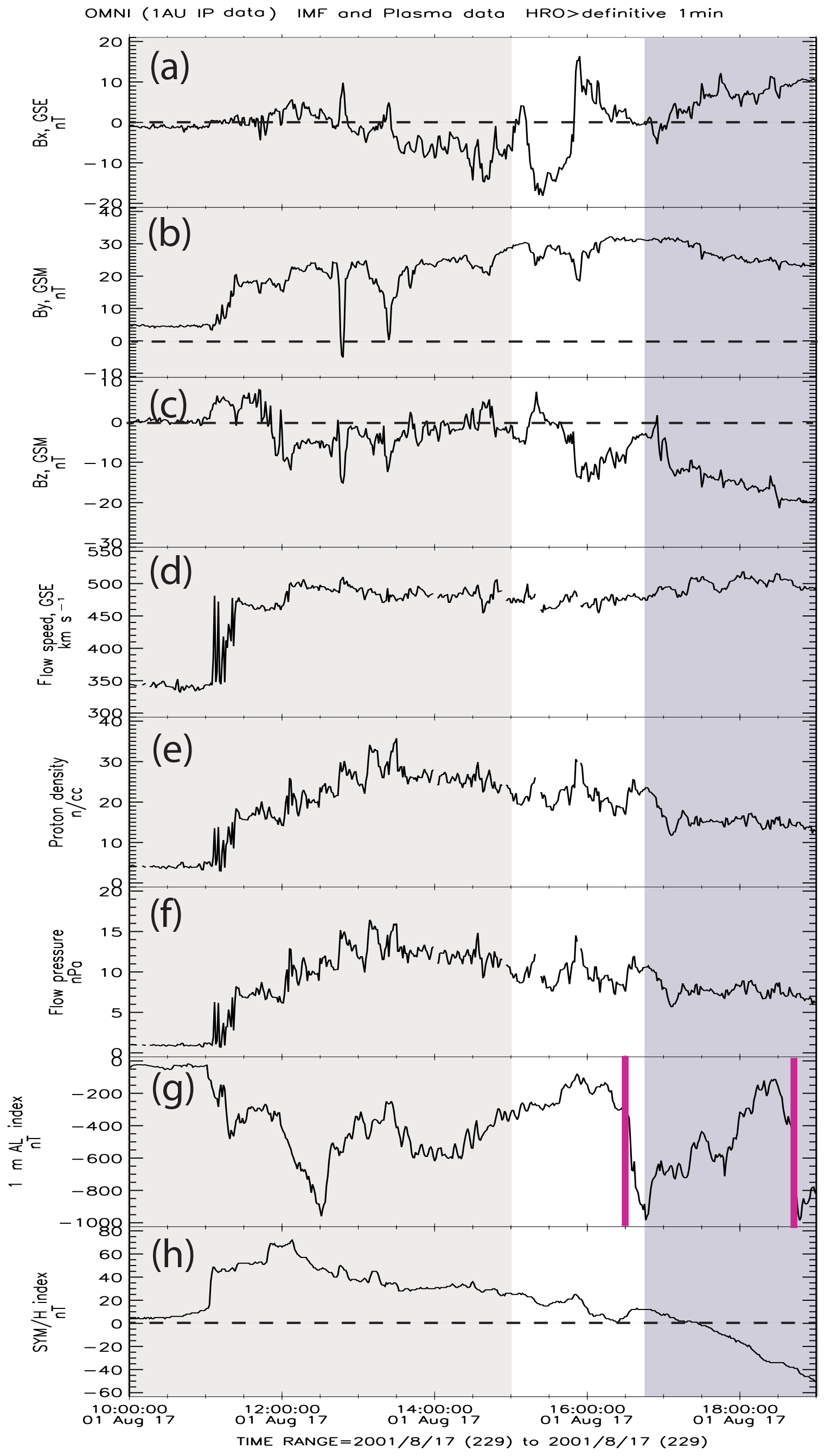
Figure 2 Solar wind (GSE coordinates), IMF (GSM coordinates) and geomagnetic indices during the passage of the CME on 17 August 2001. (a) IMF B_X, (b) IMF B_Y, (c) IMF B_Z, (d) solar wind bulk speed, (e) proton density, (f) flow pressure, (g) AL index where the two vertical red lines are the times of two substorm onsets, and (h) SYM-H index. The time period marked with light grey (10:00 to 15:00 UT) is when Polar and IMAGE were both viewing the same (northern) hemisphere, while the darker grey period from 16:45 UT to 19:00 UT is when the two satellites provided simultaneous images from the conjugate hemispheres.

4.1 A coronal mass ejection and solar wind conditions

On 15 August 2001 at 23:54:05 UT GOES 8 measured a large increase in proton flux >100 MeV (not shown), indicating a coronal mass ejection (CME). As is apparent from the time-shifted ACE data to the bow shock, a large pressure pulse was observed about 35 h later on 17 August 2001 at $\sim \mathrm{11}:\mathrm{00}$ UT (Fig. 2f) and immediately showed up in the SYM/H index (Fig. 2h) as a huge increase in the magnetopause currents as a result of a dramatic compression of the magnetosphere. The arrival of this interplanetary shock and its effect on the magnetosphere at the initial phase of the storm has been reported by others (Echer et al., 2008; Huttunen et al., 2005).

The solar wind speed (Fig. 2d) increased from 350 to 500 km s⁻¹ and stayed approximately constant for the next 8 h. The magnetic data revealed a large B_Y component (Fig. 2b) that stayed almost constant (20–30 nT) and a varying B_Z component (Fig. 2c). For the time interval with available conjugate imaging data, which we focus on in this study (16:45 to 19:00 UT), the IMF B_Y was between 30 and 24 nT and B_Z changed from 0 to −20 nT (clock angle from 90 to 135^∘). This means that during this time interval (and also for hours before that) geospace was exposed to a strongly B_Y-dominated IMF.

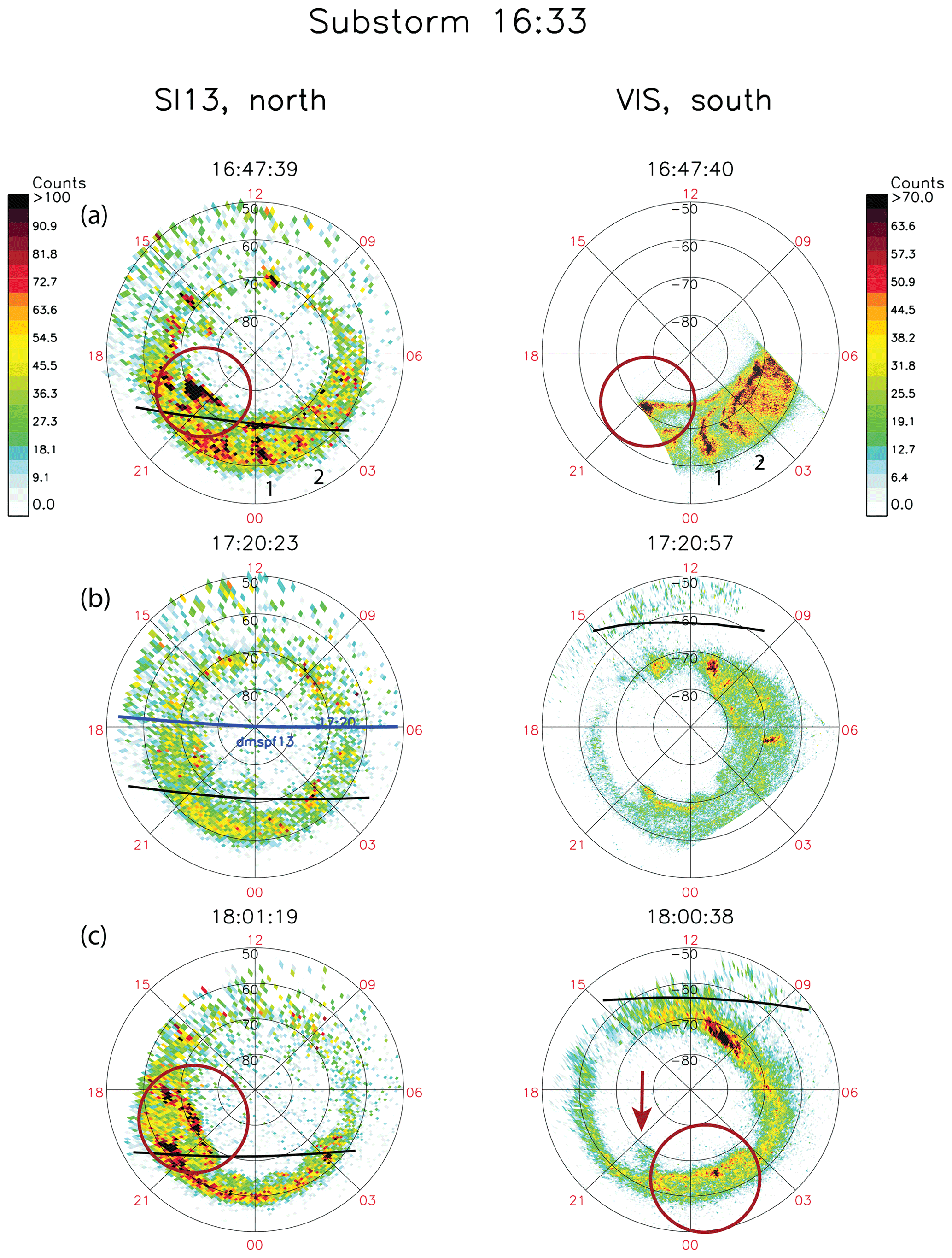
Figure 3 17 August 2001: (a–c) pairs of simultaneous (as close as possible) auroral images from Northern (left) and Southern (right) Hemispheres. All panels show SI13 and VIS. Black lines indicate the terminator at 90^∘ solar zenith angle. Features we claim are conjugate are marked with red circles and numbers in panel A. Blue line in panel (b) is the trajectory of the DMSP 13 pass in the Northern Hemisphere. Time of the first substorm is also shown.

The solar wind conditions immediately caused intense magnetic disturbances, as can be seen from both the AL index and the SYM-H index (Fig. 2g and h). The fluctuations seen around 11:00 UT in Fig. 2d, e and f are not real, but an artifact of the OMNI data time shift to bow shock. During the 2 h with simultaneous conjugate imaging there were two substorms, at 16:33 and 18:43 UT, giving us an opportunity to study how increased tail reconnection during substorm expansion phase affects the asymmetries.

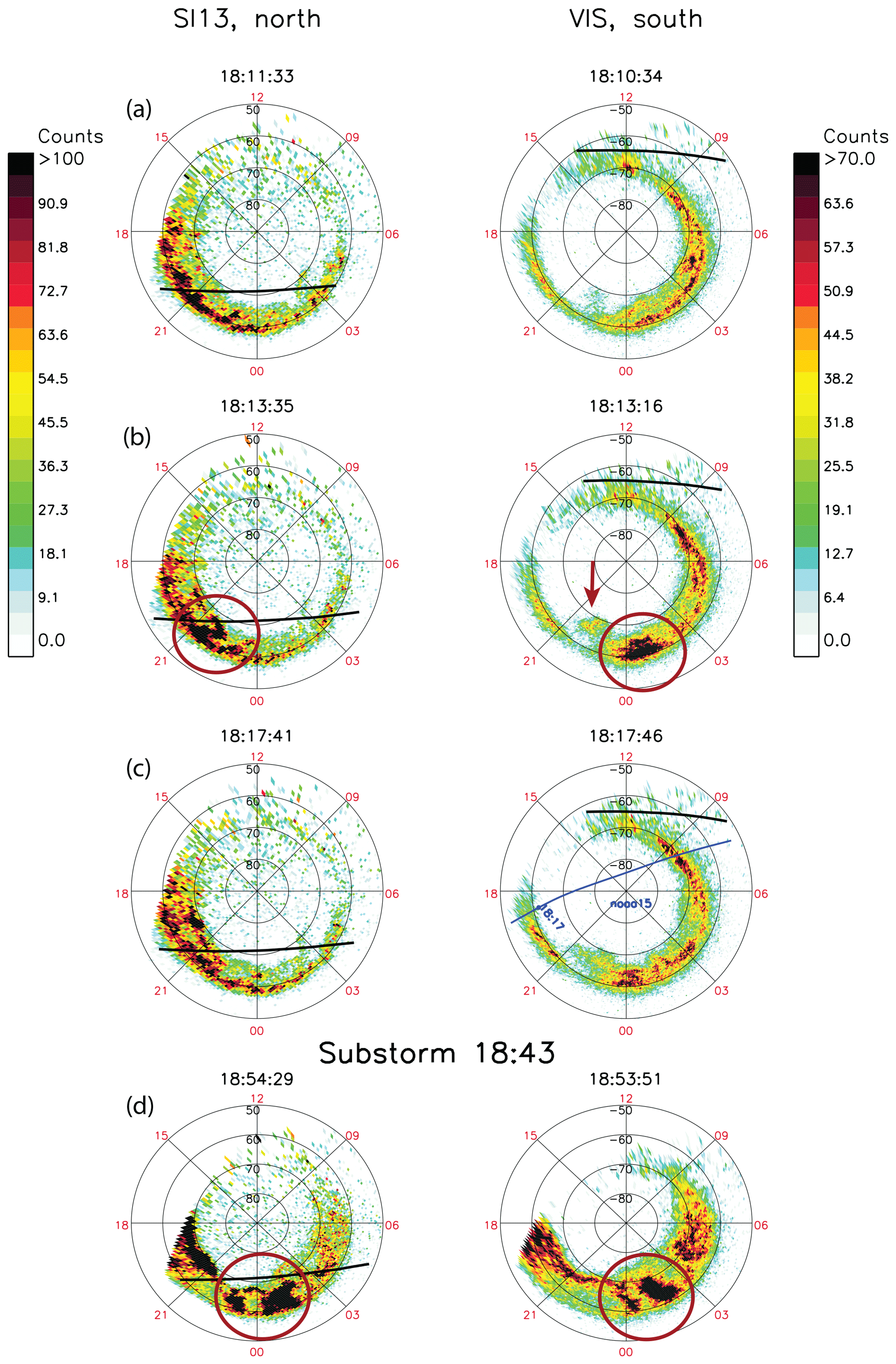
Figure 4 17 August 2001: (a–d) pairs of simultaneous (as close as possible) auroral images from Northern (left) and Southern (right) Hemispheres. All panels show SI13 and VIS. Black lines indicate the terminator at 90^∘ solar zenith angle. Features we claim are conjugate are marked with red circles. Blue line in panel (c) is the trajectory of the NOAA 15 pass in the Southern Hemisphere. Time of the second substorm is also shown.

4.2 Observations

Pairs of simultaneous images (SI13 and VIS, with the scaling established in Sect. 3) from the two hemispheres are shown in Figs. 3 and 4. Features identified as conjugate are marked with red circles. Supporting particle data are shown in Figs. 5 and 6.

In Fig. 3a we identify a hook-shaped discrete auroral feature at the poleward edge in both hemispheres at the end of the substorm expansion phase (Fig. 2g), and we interpret these as signatures of tail reconnection and consequently magnetically connected. They could be displaced by ∼1 h MLT, but as the VIS FOV prevents us from seeing the duskward side of the aurora, it could be less. We also identify two north–south features, marked 1 and 2 (Fig. 2a), seen in both hemispheres. We also believe these are conjugate and displaced by 0.5–1 h MLT.

The next pair of images (Fig. 3b) shows that the latitudinal width of the dawnside aurora is significantly larger in the Southern Hemisphere, where it extends to 80^∘ magnetic latitude at 6 h MLT. Since the auroral intensity in the SI13 is rather low, we show a DMSP 13 pass (Fig. 5) through the dawnside aurora at 6.1 h MLT in the north. The trajectory is shown by the blue line in Fig. 3b. From both the electron and proton spectrograms it is clear that the aurora does not extend beyond 74.1^∘ magnetic latitude, which is a difference of 6^∘ compared to the south. The difference in latitudinal width of the dawn aurora, although less pronounced, can also be seen in Figs. 3c, 4a, b and c.

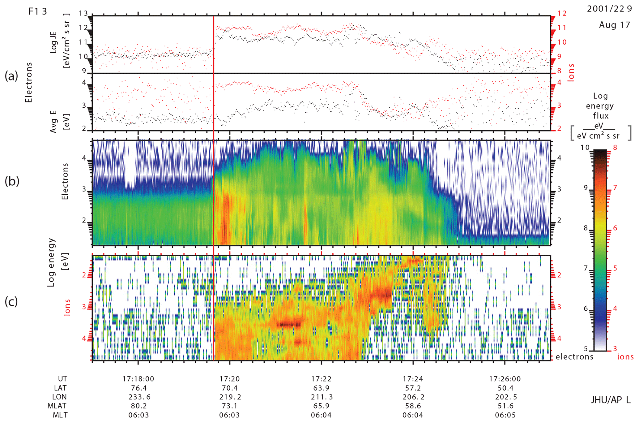
Figure 5 17 Augus 2001: DMSP 13 pass through the dawn-side aurora at 17:20 UT in the Northern Hemisphere; see trajectory in Fig. 3b. (a) Energy flux and average energies of electrons (black) and protons (red). (b) Differential energy flux of electrons. (c) Differential energy flux of protons. Red vertical line marks the poleward edge of precipitation at 74.1^∘ magnetic latitude.

Now we return to Fig. 3c, where we identify discrete auroral features at the poleward edge of the aurora (at the open–closed boundary – OCB) and we interpret these as signatures of tail reconnection. They are displaced ∼4 h MLT and their poleward edges are about 4^∘ different in magnetic latitude. We have also pointed to a weak auroral feature in the Southern Hemisphere at ∼22 h MLT (red arrow) which could be interpreted as being conjugate to the eastward edge of the poleward feature in the Northern Hemisphere. One could then argue that it is a sensitivity issue that Polar VIS does not see the entire poleward arc from 18 to 22 MLT. However, there are several arguments for this not being the case, the first being the dynamical change that occurred from 18:11 (Fig. 4a) to 18:13 UT (Fig. 4b) when there is a sudden brightening at the eastward edge of the poleward feature in the north. In the Southern Hemisphere it is not the weak auroral feature marked with the red arrow in Fig. 4b (VIS) that brightened up, but the region we identified in Fig. 3c to be conjugate. When two relatively large regions brighten up simultaneously in the two hemisphere, it is a strong indication of having a common source region in the magnetosphere. To further support our interpretation we show a NOAA 15 pass 4 min later at 18:17 UT (Fig. 6) through the dusk-side aurora in the south. The trajectory is shown by the blue line in Fig. 4c. These electron data clearly indicate that there is no auroral precipitation poleward of $-\mathrm{62.2}{}^{\circ }$ magnetic latitude, while the northern aurora extends to about 70^∘ magnetic latitude at 18.6 MLT, as seen in Fig. 4c. It is not a camera sensitivity issue. There is no poleward auroral feature at 18–21 MLT in the Southern Hemisphere. In Sect. 4.7 we show that the convection pattern in the Northern Hemisphere, derived from measurements only and independent of the imaging data, locates the region of flux transport across the OCB (indicative of tail reconnection) exactly where the poleward auroral feature is bright. We will also show that the OCB is not moving equatorward during this interval, further supporting that there is indeed flux transport across the OCB in this region.

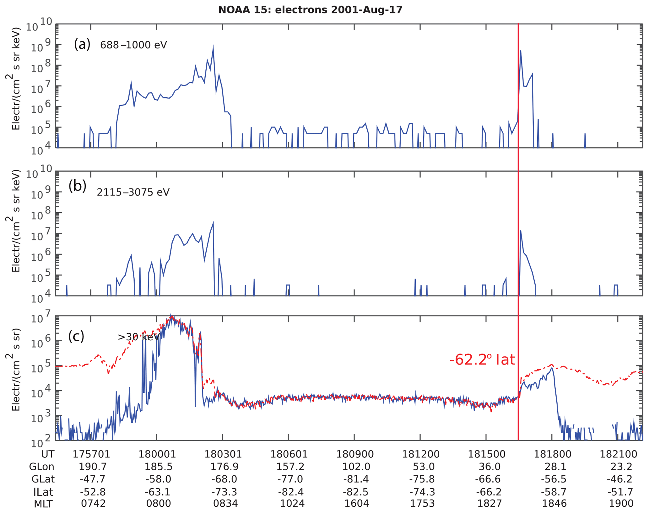
Figure 6 Particle measurements from NOAA 15 pass in the Southern Hemisphere on 17 August 2001; see trajectory in Fig. 4c. It passed through the dusk-side aurora at 18:17 UT. (a) Electron flux: 688–1000 eV. (b) Electron flux: 2115–3075 eV. (c) Electron flux: ≥30 keV, where the blue line shows electrons within the loss cone and the red line shows the locally mirroring electrons. The red vertical line shows the poleward edge of precipitation at $-\mathrm{62.2}{}^{\circ }$ magnetic latitude.

Table 1 Summary of asymmetric features identified in Figs. 3 and 4.

Our last pair of images (Fig. 4d), 10 min after the second substorm, shows relatively large north–south discrete auroral features that are not identical but have similar shapes. These features are in darkness in both hemispheres, so conductivity differences should not be an issue. Based on how similar they are, and that there are no other features that could confuse the link we make between these features, we interpret these also to have a common magnetospheric source region, and consequently they are magnetically connected. The displacement is about 1–1.5 h MLT.

Figure 7 Field line tracing from one hemisphere to the other using the Tsyganenko 2002 model. (a) Blue symbols indicate the starting tracing points in the Northern Hemisphere. Filled and open symbols are used for the poleward and the equatorward edge of the aurora, respectively. In panels (b) and (c) blue (red) symbols mark the footprint in the Northern (Southern) Hemisphere for tracing from north to south using different input values (see text for explanation). The blue symbols are at the same locations in all panels.

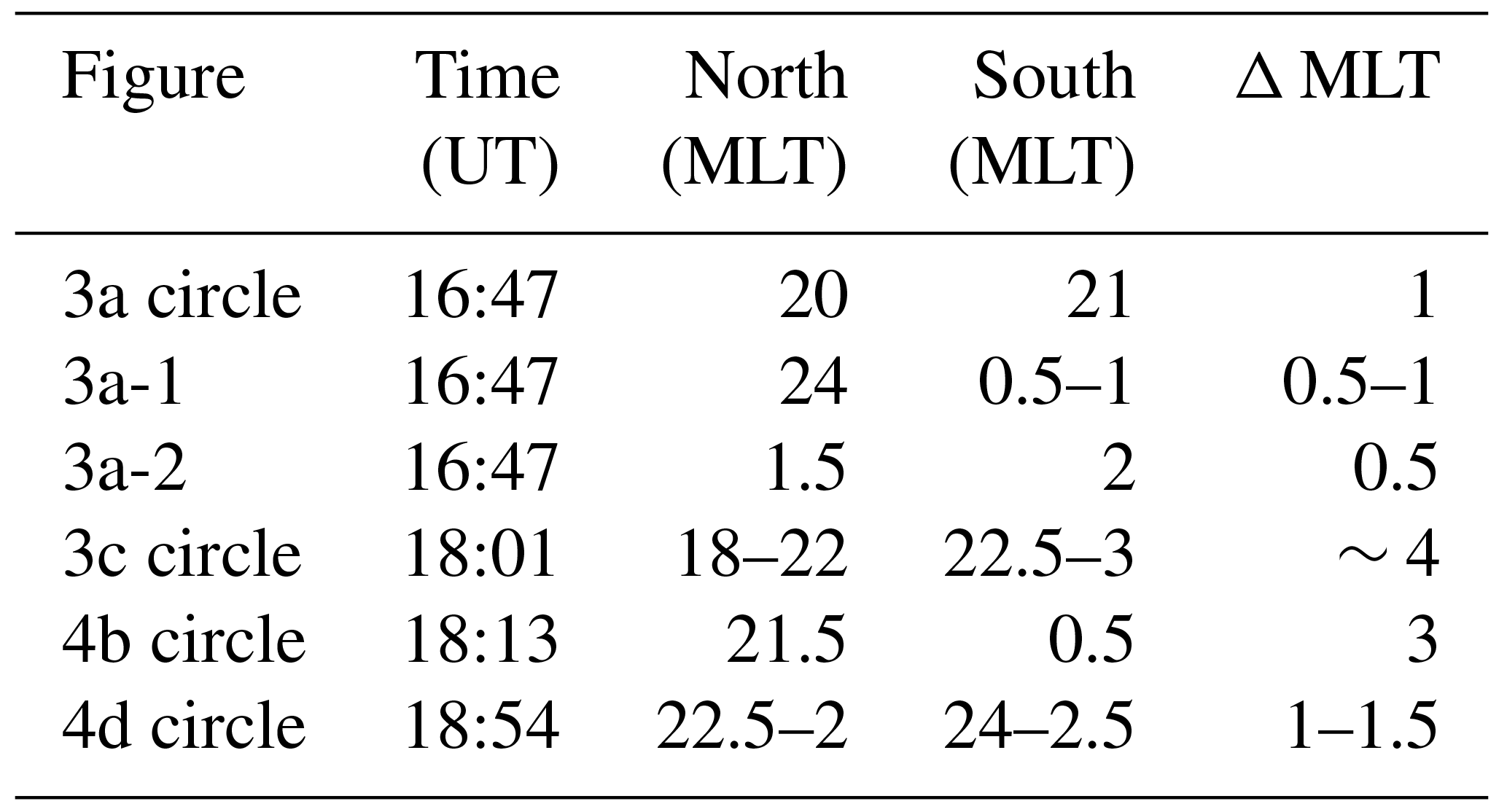
In Table 1 we have summarized the asymmetries identified in Figs. 3 and 4. These will be shown by diamonds in Fig. 10.

4.3 Comparison with model

As was seen in Fig. 3c the conjugate auroras in the two hemispheres are displaced by about 4 h MLT. From careful inspection of auroral features before and after we are fairly confident that this interpretation is correct. In order to compare our observations with an empirical model, we have used the Tsyganenko 2002 (T02) model to investigate the magnetic mapping between the hemispheres (Tsyganenko, 2002a, b). In addition to the tilt angle of 23^∘ the input parameters (as seen from Fig. 2) should have been as follows: dynamic pressure, 8 nPa; solar wind speed, 500 km s⁻¹; Dst, −17 nT; IMF B_Y, 26 nT; and IMF B_Z, −14 nT. As these IMF conditions are rather extreme, especially the dynamic pressure, B_Y and B_Z, and in a range very poorly represented in the database used to generate the T02 model, the output would be an extreme extrapolation of the model. We have therefore reduced the input values to the following: dynamic pressure, 2 nPa; IMF B_Y, 10 nT; and IMF B_Z, −5 nT (clock angle is unchanged). The others were kept as measured (Fig. 7b). In addition we show the results for input values of dynamic pressure of 2 nPa, but with 50 % larger IMF B_Y (15 nT) and IMF B_Z (−8 nT; Fig. 7c) and still the same clock angle. The latter input values are used to show how the extrapolation of the model leads to even larger asymmetries and serves to illustrate the combined effect of large IMF B_Y and large tilt angle. The starting points in the Northern Hemisphere are chosen as far north as possible (69^∘ magnetic latitude) in order to return closed field lines within the region where the model is valid. We have chosen the point on the westward side of the poleward arc; see filled blue symbols in Fig. 7a. The starting points at the equatorward edge are marked with open blue symbols. The red symbols in Fig. 7b and c are the mapping locations in the Southern Hemisphere. The tracing shows a large asymmetry on the poleward edge of the aurora (about 1.5 h MLT in Fig. 7b and 2.5 h MLT in Fig. 7c) and close to no asymmetry at the equatorward edge. This increase in asymmetries for increasing IMF B_Y, but at the same clock angle, is expected from our understanding of how asymmetries are produced by asymmetric loading of magnetic flux in the lobes, and how asymmetries are reduced as the flux tubes move toward the Earth (Tenfjord et al., 2015). We want to emphasize that we do not expect the T02 model to reproduce our findings exactly, but it gives qualitative support for observing large asymmetries at the poleward edge of the auroral oval at dusk.

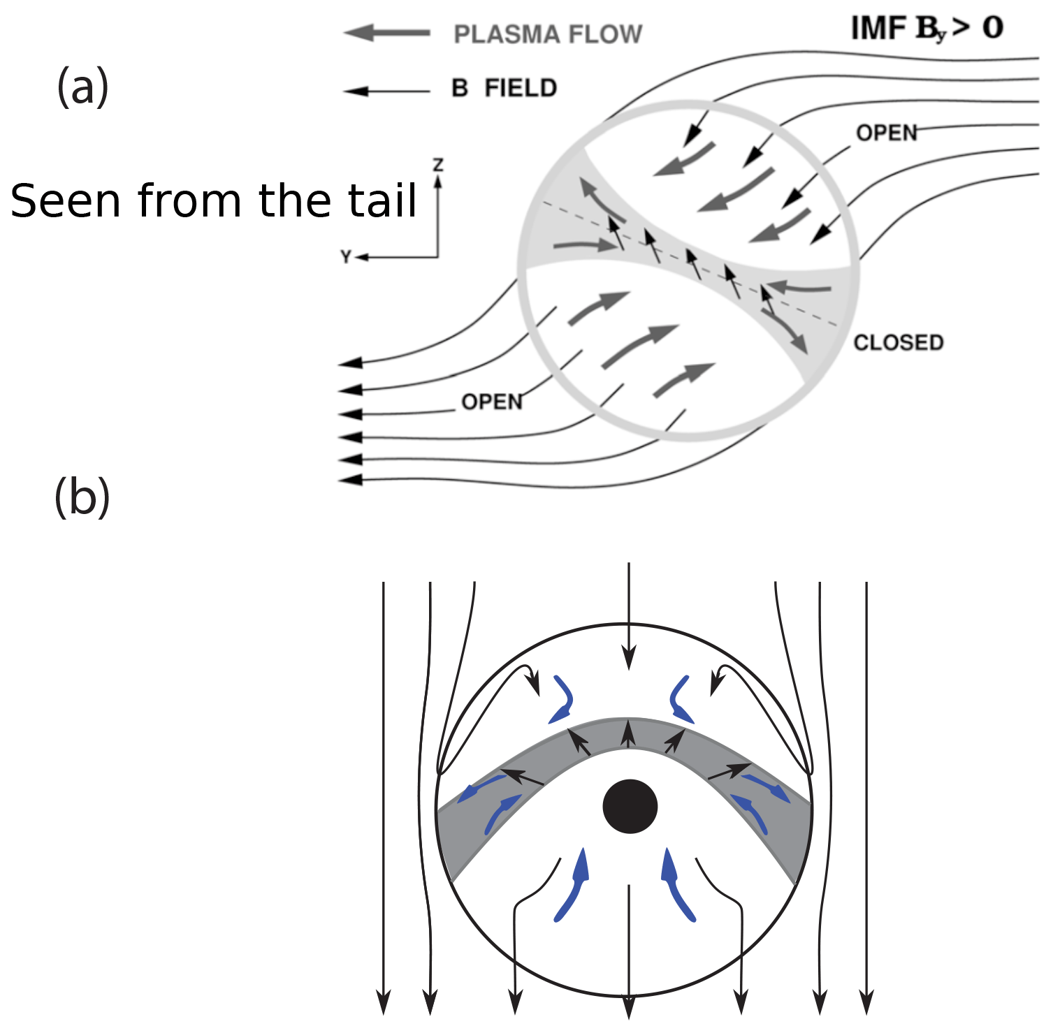
Figure 8 Plasma flow and magnetic fields in the mid-tail (YZ plane) as seen from the tail. The white regions are the lobes and the shaded grey regions are the plasma sheet in the closed magnetosphere. (a) The effect of IMF B_Y>0, similar to Fig. 3a in Liou and Newell (2010), which was adapted from Khurana et al. (1996). (b) The effect of large tilt angle and warping of the tail (Tsyganenko, 1998), similar to Fig. 3b in Liou and Newell (2010). The plasma flow (or the motion of magnetic flux tubes) are shown as thick grey and blue arrows in (a) and (b), respectively. Magnetic fields are shown as thin black arrows.

4.4 Why such large asymmetries?

As suggested by Hau and Erickson (1995) and Khurana et al. (1996) a B_Y component will be induced in the plasma sheet (closed magnetosphere) as a result of asymmetric loading of magnetic flux to the lobes and subsequent plasma flow (or motion of magnetic flux tubes), as shown in Fig. 8a. This effect is apparent in the Tsyganenko model (Østgaard et al., 2005) and MHD models (Tenfjord et al., 2015). For further details about how B_Y is induced in the closed magnetosphere we refer to Tenfjord et al. (2015), where this is explained in great detail, both theoretically and by showing MHD model results. As shown in Fig. 8b there will be an additional effect of a large tilt angle. For positive tilt angle the central plasma sheet will move upward but less so towards the flanks. This configuration has been described as warping of the plasma sheet (Gosling et al., 1986). Similar to the asymmetric loading of magnetic flux in the lobes leading to plasma flow and induced B_Y, the warping of the tail also causes asymmetric flow of magnetic flux towards the plasma sheet and induces B_Y components in the closed magnetosphere of opposite polarity in dawn and dusk (Liou and Newell, 2010; Tsyganenko, 1998).

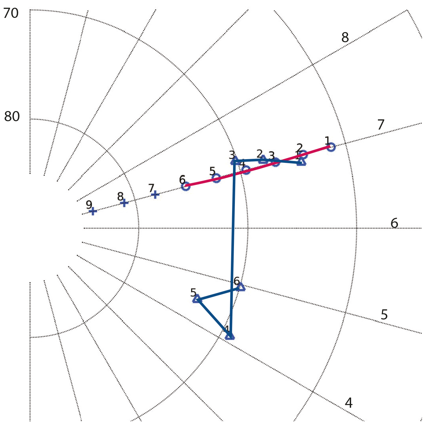
Figure 9 Tracing field lines from south (red), 62 to 75^∘ at 7 MLT, to north (blue) using the LFM model. The field lines from 70 to 75^∘ latitude in the south map to an azimuthally extended region in the north.

We interpret the large displacement of the footpoints for conjugate field lines that we observe (3–4 h MLT) in the dusk sector to be the combined effect of large IMF B_Y and large tilt angle per second of warping. In the dawn sector the warping effect will reduce the effect of IMF, induced B_Y and this is consistent with what we see in Fig. 3a for feature 1 and 2.

4.5 Why latitudinal wider aurora in the southern dawn?

As we pointed out in Sect. 4.2 the auroral oval is about 6^∘ wider in the southern dawn compared to northern dawn (Fig. 3b). We interpret this also to be an effect of the asymmetric loading of flux (due to IMF B_Y) and maybe an additional effect of enhanced lobe pressure in the north from warping for large tilt (Fig. 8b). The effect is only on the poleward side of the aurora, while the equatorward boundary of the aurora is at similar latitudes in the two hemispheres. If we assume that the dawn aurora is on conjugate field lines the magnetic flux in the auroral oval has to be conserved. This means that the poleward segment of the aurora in the south has to map to an azimuthally extended region in the north. In order to justify such an interpretation we ran the Lyon–Fedder–Mobarry (LFM) MHD model (Lyon et al., 2005; Merkin and Lyon, 2010) with boundary conditions similar to the 17 August event. From Fig. 9 we see that field lines from 70 to 75^∘ latitude (at same longitude) map to an azimuthally extended region in the north. At least qualitatively, the LFM model supports this interpretation.

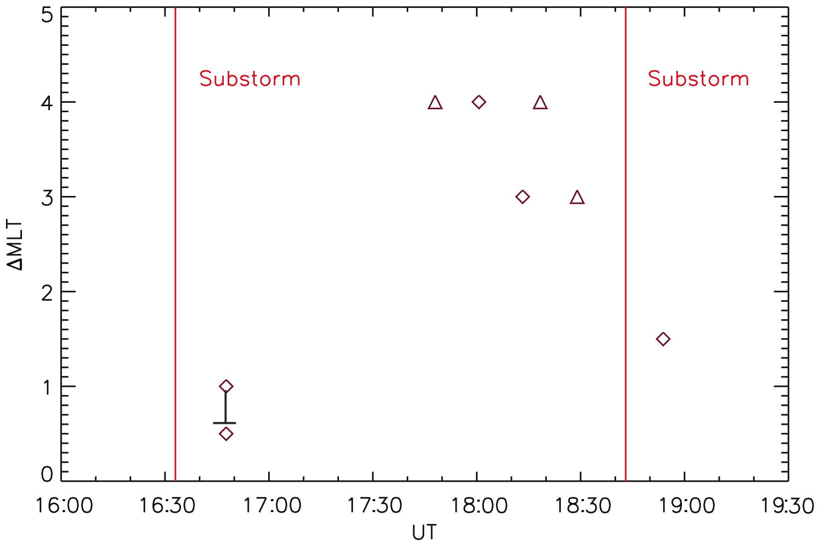
Figure 10 Time evolution of asymmetric conjugate auroral features. Diamonds are auroral asymmetries identified from Figs. 3 and 4 and listed in Table 1, while triangles are identified from images not shown, but which can be found in auxiliary material. The red vertical lines are the times of the substorms.

4.6 Time evolution of asymmetries and the role of substorms

In Fig. 10 we display the evolution of asymmetric locations of conjugate auroral features in the two hemispheres. For the first point (at 16:48 UT) we show both the feature within the red circle in Fig. 3a (Δ MLT∼1, with an approximate uncertainty as explained in Section 4.2) as well as the equatorward tip of features 1 and 2 (Δ MLT=0.5). We see that the asymmetries are smaller after each substorm and build up to 3–4 h MLT between the substorms. We interpret this as follows. It is well established by observations that the lobe pressure increases before the substorm and decreases in less than 1 h after substorm onset (Caan et al., 1975). The accumulation of open flux before the substorm causes the magnetosphere to inflate and the tail magnetopause to flare outward. This increases the cross-sectional area that the magnetosphere presents to the solar wind and leads to a buildup of pressure in the tail. When this loading is asymmetric, due to the large IMF B_Y, the induced B_Y increases before the substorm. As has been shown statistically by Juusola et al. (2011) the rate of fast bursty bulk flows increases significantly during the substorm expansion phase (see their Fig. 4). As bursty bulk flows are signatures of tail reconnection, it means that open magnetic flux is efficiently closed in the tail and the flaring angle decreases. This results in a smaller cross-sectional area of the magnetosphere leading to a lower pressure in the tail. The asymmetric lobe pressure that induced the asymmetries in the first place is effectively reduced when tail reconnection increases. Contrary to what has been suggested by others (Motoba et al., 2010; Stenbaek-Nielsen and Otto, 1997; Østgaard et al., 2004), increased tail reconnection does not add any B_Y component into the closed magnetosphere, but by reducing the asymmetric lobe pressure rather acts to reduce the B_Y. Reduction of IMF B_Y-related asymmetries during the substorm expansion phase has been observed both in conjugate auroral images (Østgaard et al., 2011a) and in convection patterns (Grocott et al., 2010).

4.7 Convection pattern

Finally, as outlined in Sect. 3, we will use all available data to find the most likely convection patterns as well as the location of the open–closed boundaries in the two hemispheres for the period when we observe large asymmetry. The convection patterns are derived independently of the imaging data. Although 18:01 UT is the time when the asymmetries are most clearly identified, we have chosen the time interval around 17:47 UT for this purpose, because we have data from two SuperDARN radars with overlapping FOV to help us draw the convection pattern in the Southern Hemisphere. The bright poleward auroras indicative of tail reconnection are still clearly seen in both hemispheres. In the Northern Hemisphere we also have good data coverage at this time and can use both SuperDARN line of sight, a DMSP SSIES and SuperMAG data as input to the spherical elementary convection cell technique described in Sect. 3. We also want to point out that we have good data coverage in the Northern Hemisphere both before and after 17:47 UT and the derived convection pattern does not change, when using data input before and after that time.

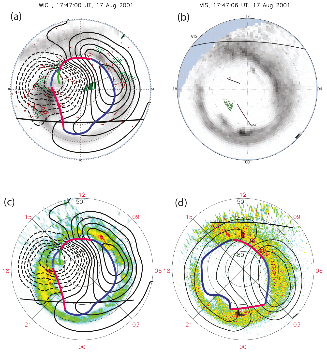
Figure 11 Convection patterns in the two hemispheres at 17:47 UT, 17 August 2001. (a) SuperDARN line of sight (green dots), SuperMAG (brown arrows) and DMSP SSIES (green arrows) are used to estimate the global convection pattern in the Northern Hemisphere. Blue and red lines indicate the open–closed boundary, where the red lines are dayside and nightside reconnection regions. The green line indicates lobe reconnection. (b) Southern Hemisphere where a few vectors from SuperDARN are available (green arrows). (c) Similar convection pattern to that from panel (a) overlaid on the auroral intensities. (d) Convection pattern and open–closed boundary in the southern pattern drawn by hand, guided by the few available SuperDARN vectors (b) and auroral features of dayside and nightside reconnection.

4.7.1 Convection pattern in the Northern Hemisphere

In Fig. 11a we show the convection patterns, derived from measurements only, in the Northern Hemisphere and these reveal a relatively small “orange” cell in the dusk and a large “banana” cell in the dawn. We use the poleward boundary of the aurora as a proxy for the open–closed boundary (Laundal et al., 2010), which is marked with blue and red lines. The red lines indicate where plasma, according to the derived convection pattern, flows with highest intensity across the OCB. We can identify dayside reconnection between 11 and 15 MLT that opens magnetic flux and tail reconnection between 18 and 22 MLT that closes magnetic flux. The convection pattern also indicates that there might be weak flows across the OCB dawnward of 22 MLT. To check whether the flows between 11–15 and 18–22 MLT seen in Fig. 11a are really flows across the OCB and not only a motion of the OCB itself, we show, in Fig. 12, the time evolution of the OCB in the two hemispheres derived quantitatively from IMAGE WIC (450 counts) in the north and Polar VIS (5 counts) in the south. From Fig. 12a it can be seen that the OCB in the Northern Hemisphere does not move with the flow in the 11–15 and 18–22 MLT sectors from 17:45 to 18:01 UT, but is rather stable, which means that there is indeed flux transport across the parts of the OCB marked as red lines. For the region of tail reconnection (18–22 MLT in Fig. 11a), this is exactly where we observe the bright poleward feature in the north, giving independent support for our interpretation that the poleward auroral feature is indeed a signature of tail reconnection (Sect. 4.2).

In Fig. 11a we have marked lobe reconnection by a green line from 15 to 17.5 MLT. The observational support for lobe reconnection is the auroral spot (Milan et al., 2000) seen at 17.5 MLT in Fig. 11a and c between 75 to 80^∘ magnetic latitude, clearly detached from the oval. This feature $>\mathrm{75}{}^{\circ }$ magnetic latitude is present in almost all the images since the arrival of the CME at 11:00 UT. It is seen during the 5 h of imaging data from the same hemisphere and from 16:18 UT when we have images from conjugate hemispheres (Fig. 3a). The spot becomes faint at 17:15 UT but reappears between 17:40 and 17:50 UT (Fig. 11c). Fig. 13 shows IMAGE WIC images (Northern Hemisphere) from 16:19 to 16:49 UT, where this spot is seen clearly detached from the auroral oval in all 10 images (see also the video, uploaded in the Supplement). Frey et al. (2003b, 2004) statistically explored the characteristics of this high-latitude dayside aurora (HiLDA) and concluded that the major driving process was high-latitude (lobe) reconnection and that it occurred preferentially in the summer hemisphere.

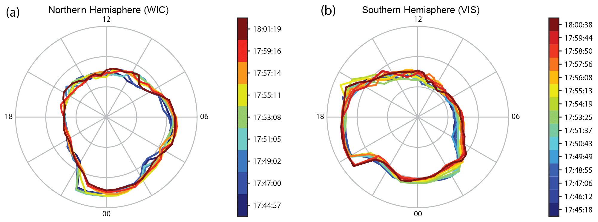
Figure 12 Open–closed boundaries derived from IMAGE WIC images in the north and Polar VIS in the south from 17:45 to 18:01 UT on 17 August 2001.

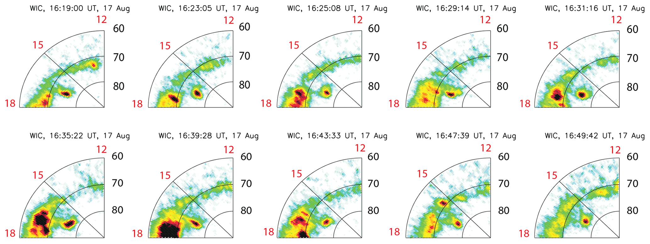
Figure 13 IMAGE WIC images. The auroral spot $>\mathrm{75}{}^{\circ }$ magnetic latitude, clearly detached from the auroral oval and indicative of lobe reconnection, is seen from 16:19 to 16:49 UT, 17 August 2001.

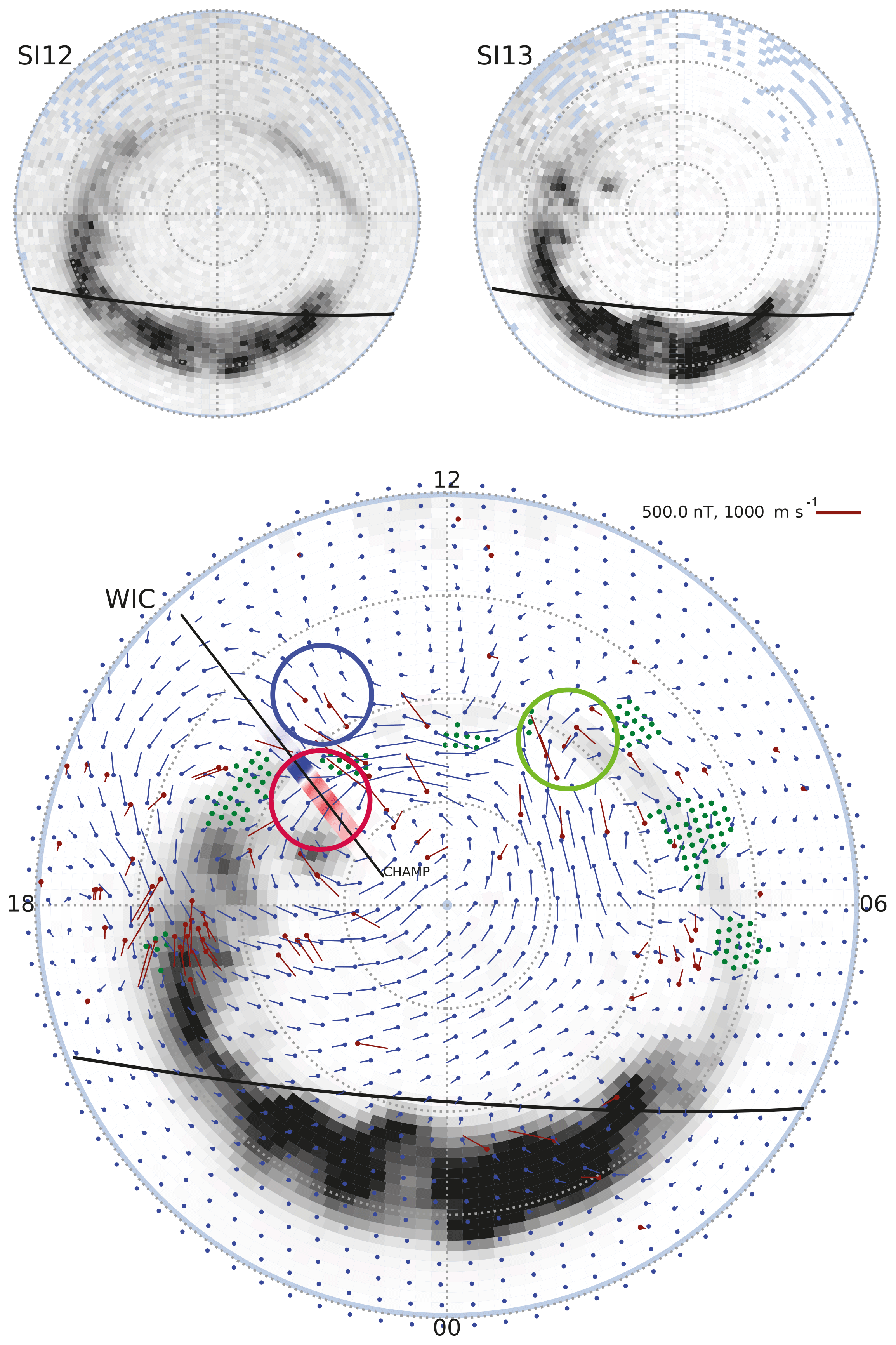
Figure 14 Auroral images from the Northern Hemisphere at 16:31 UT, 17 August 2001. (a) SI12, (b) SI13 and (c) WIC with derived currents from CHAMP pass. Red (blue) is upward (downward) currents. The green dots indicate locations of SuperDARN backscatter. SuperMAG equivalent currents are shown with brown vectors. The scale of the convection and magnetic field perturbations are shown in the top right corner of the WIC image. The location of the sunlight terminator is indicated by a black line. Derived convection patterns are shown by blue vectors. The three circles mark the flows discussed in the text.

To further support that the auroral spot is associated with lobe reconnection we show the images as well as the derived convection pattern from the Northern Hemisphere at 16:31 UT (Fig. 14). The spot is seen in SI13 and WIC but not in SI12, which means that it is produced by electron precipitation. This is further supported by the derived upward current from CHAMP data. The derived convection shown by blue arrows in Fig. 14 indicates sunward flow at very high latitudes (75^∘, marked with a red circle), just where we see the spot and the upward field-aligned current from CHAMP. The LFM model also predicts a strong upward current on open field lines between 70 and 80^∘ at 17–18 MLT (not shown).

Flow across the OCB (Fig. 14, marked with a blue circle) indicating dayside reconnection is seen around 15 MLT and $<\mathrm{70}{}^{\circ }$ with downward current (CHAMP) and proton precipitation (SI12 image). Flow across the OCB is also seen at 11 MLT and $<\mathrm{70}{}^{\circ }$ (green circle), consistent with the dayside reconnection region that we have indicated by the red line in Fig. 11a. Since the flow between 11 and 13 MLT is mostly along the OCB, the flows seen within the green and blue circle indicate split reconnection X lines, similar to what was reported by Chisham et al. (2002) during similar IMF conditions. The equatorward convection just outside the auroral oval near noon is probably an artifact of the inversion, since the solution there is relatively unconstrained by observations compared to surrounding regions (SuperDARN backscatter locations are indicated by green dots). To have lobe reconnection under such B_Y-dominated IMF conditions has been reported by others (Nishida et al., 1998; Sandholt et al., 1998) and especially in the Northern Hemisphere for such a large tilt angle (Crooker and Rich, 1993). The combination of dayside reconnection and lobe reconnection was suggested by Reiff and Burch (1985) for weakly southward IMF with dominated B_Y, which is exactly the IMF conditions we have. Compared to their Fig. 1, our red line corresponds to their region L to M, and our green line (lobe reconnection) to their region between M and H. The statistical studies by Frey et al. (2003b, 2004) also support our interpretation. In Fig. 11c we show the same convection pattern and open–closed boundary onto the WIC color image from 17:47:00 UT.

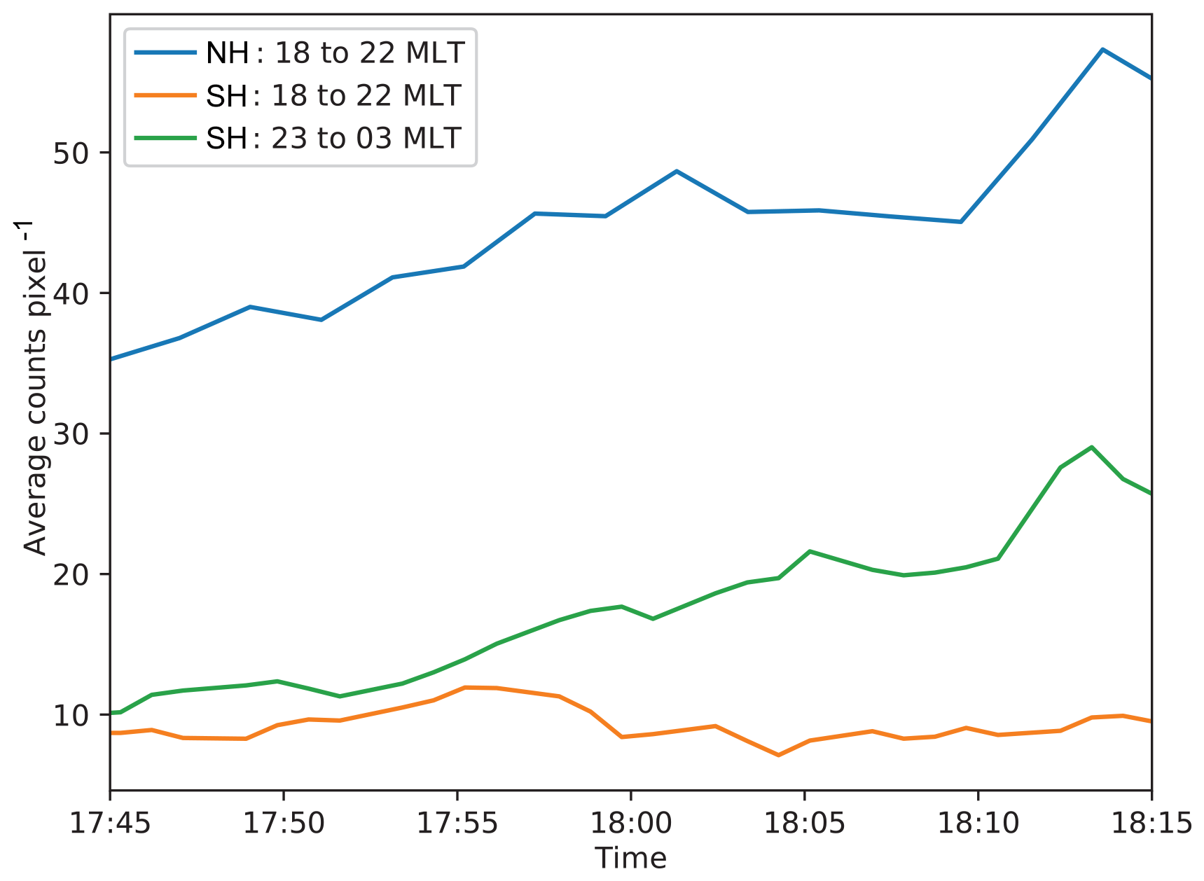
Figure 15 Average counts per pixel between 55 and 75^∘ magnetic latitude in selected MLT sectors from 17:45 to 18:15 UT on 17 August 2001. Blue line: Northern Hemisphere 18–22 MLT; orange line: Southern Hemisphere 18–22 MLT; and green line: Southern Hemisphere 23–3 MLT.

4.7.2 Convection pattern in the Southern Hemisphere.

Now we return to Fig. 11b and c to suggest a possible convection pattern in the Southern Hemisphere. In this hemisphere there are too few data points to apply the spherical elementary convection cells technique. However, we can use the auroral features (Fig. 11d) combined with the convection vectors (green arrows in Fig. 11b) measured by two SuperDARN radars with overlapping FOV to determine the OCB and suggest a possible convection pattern. Firstly, we notice the auroral signature of dayside reconnection between 9 and 12 MLT. This is even more clear in the VIS image from 18:01 UT (Fig. 3c). Secondly, as we argued in Sect. 4.2, the discrete poleward feature in the Southern Hemisphere between 22 and 2 MLT is the auroral signature of tail reconnection in this hemisphere. As for the Northern Hemisphere, we mark the OCB at the poleward side of the auroral oval (see also Fig. 12b) with a red line indicating reconnection regions and a blue line for the rest of the OCB. With these constraints and SuperDARN vectors to guide us we have drawn one possible solution for the convection pattern overlaid on the VIS image from 17:47 UT (Fig. 11d). We should mention that there exists a SuperDARN convection map (see their web page), which supports the locations of dayside and tail reconnection. However, there are no data in the dawnside and the convection reversal in this map is not consistent with the poleward edge of the auroral in this hemisphere. In the Southern Hemisphere we do not see any auroral features that could indicate lobe reconnection. We believe that this is due to the very large tilt angle (23^∘), which makes the northern lobe more exposed to the IMF than the southern lobe, and can explain why we see lobe reconnection in one hemisphere and not in the other. This is in agreement with Crooker and Rich (1993), who suggested that lobe reconnection is a summer phenomenon that can occur in one hemisphere only, and Frey et al. (2003b, 2004), who also found the HiLDA to be a summer phenomenon.

4.8 Alternative interpretation

Let us now consider that the features we identify as being asymmetric are not conjugate, but result from either ionospheric processes or have different sources in the magnetosphere. We have identified three types of features:

1. intensification of the aurora close to the open–closed boundary, often called poleward boundary intensification (PBI), Fig. 3a and c;

2. large-scale sudden brightening (Fig. 4b);

3. large-scale bright auroral structures with similar shapes (Fig. 4d).

PBIs are often associated with tail reconnection. However, in a recent paper Ohtani and Yoshikawa (2016) propose a mechanism where the PBIs result from convection flow shears in the ionosphere. The idea is that when “fast polar cap flows”, which is the dynamical driver in this scenario, encounter the poleward boundary of the aurora the conductivity gradients associated with this aurora force the flux tubes to move along rather than across the boundary. This results in a flow shear which creates a pair of upward–downward currents and consequently auroral intensification at the upward leg. However, as these “fast polar cap flows” are open flux tubes dragged across the polar cap by the solar wind, a fast flow approaching the OCB also means an increase in inflow in the tail reconnection region. Such a flow can only be sustained if field lines reconnect in the magnetosphere. We do not question that the fast flows lead to flow shears in the ionosphere and that this may explain the changes in auroral intensities, but we will argue that the ultimate driver for these “fast polar cap flows” is reconnection at the tailward end of these flux tubes. These “fast polar cap flows” and associated auroral intensifications are ionospheric signatures of enhanced reconnection and consequently conjugate.

Let us now assume that the poleward auroras in Fig. 3c have two different magnetospheric sources and the magnetosphere is less asymmetric or even symmetric. We will focus on the 18–22 MLT region. In this region we would then need a mechanism that launches particles (preferentially electrons) close to the OCB only into the Northern Hemisphere. Fig. 6 clearly shows that there is a complete absence of particle precipitation in the Southern Hemisphere at 18.6 MLT at high latitudes. We are not aware of any theory that can explain a relatively high flux of particles into one hemisphere and total lack of particles into the other hemisphere from the same large source region (about 4 MLT hours) in the magnetosphere.

To further examine whether the 18–22 MLT sector in the two hemispheres might be conjugate we show (Fig. 15) the average counts per pixel between 55 and 75^∘ magnetic latitude in this sector. No scaling between cameras is applied as we only want to explore the intensity changes in each sector. The Northern Hemisphere is shown by the blue line and Southern Hemisphere by the orange line. The linear Pearson correlation coefficient is only 0.002. We also show the average counts per pixel in the 23–3 MLT sector in the Southern Hemisphere (green line). The correlation coefficient between the blue and green line (that is the two sectors we claim to be conjugate) is 0.95. These sectors show a steady increase and a spike at 18:13 UT, which is the sudden brightening (seen in Fig. 4b).

An often-cited mechanism for differences in auroral intensities is the suppression of discrete aurora by sunlight (Newell et al., 1996). The poleward aurora seen in Fig. 3c in the 18–22 MLT sector in the north is indeed in sunlight, but much brighter than the (missing) aurora in the southern darkness between 18 and 22 MLT. This is opposite of what Newell et al. (1996) predict.

We also want to point to the convection pattern (Figs. 11 and 14) that independently of imaging data shows strong convection across the OCB (reconnection) exactly where we see the poleward aurora in the north. If we assume that the northern 18–22 MLT region maps to the 18–22 MLT region in the south (symmetric magnetosphere) we would expect to see at least some “weak” signatures of this tail reconnection in the south. We therefore find it quite unlikely that the tail reconnection region maps to 18–22 MLT in the Southern Hemisphere, but find strong support for this to be the case in the Northern Hemisphere. We conclude that both particle data (Fig. 6) and convection pattern (Figs. 11 and 14) contradict the hypothesis of a symmetric magnetosphere. What could then be questioned is whether the tail reconnection maps to the 23–3 MLT region in the south. Unfortunately, we do not have convection data showing flow across the OCB in this region, but it is hard to envision any other auroral features that could indicate tail reconnection in the south.

The sudden brightening seen in Fig. 4b is about 3 h MLT displaced in the two hemispheres. The aurora in both hemispheres brightens up in less than 2 min and is accompanied by a 100 nT decrease in the AL index. Although the brightening does not expand into typical substorm bulges, they both have extensions of 6–8^∘ latitude and more than 1 MLT in azimuth. Mapped into the plasma sheet (not shown) they cover huge regions (ΔY: 4–5 R_E and ΔX: ∼10 R_E). If these are two separate regions, we have one large magnetospheric source region that only launches electrons into the Northern Hemisphere (and nothing to the Southern Hemisphere) and another large magnetospheric region that, at the same time, only launches electrons into the Southern Hemisphere (and nothing into the Northern Hemisphere). Again, we are not aware of any theory that could explain such asymmetric behavior of the magnetosphere. Alternatively, there is a large region in the magnetosphere that maps to a 5 h MLT sector in the ionosphere (21–2 MLT) and that the western part launches electrons into the Northern Hemisphere and the eastern part only launches electrons into the Southern Hemisphere. The same scenario could then be used for all substorm onset studies, and we are not aware of any studies that have found support for such an interpretation. Although not very likely, we cannot rule out this possibility.

Finally, if we assume the auroral features in Fig. 4d to have different magnetospheric source regions, we end up with the same dilemma as for the sudden brightening. One source region only launches electrons into one hemisphere and another only into the other hemisphere.

5 Conclusions

The magnetic storm on 17 August 2001 has given us a unique opportunity to study the dynamical behavior of the asymmetric geospace. The magnetic storm occurred at 11:00 UT on 17 August 2001. Solar wind had high pressure, IMF was dominated by a large B_Y of 20-30 nT, and clock angle varied between ∼90 and $\sim \mathrm{135}{}^{\circ }$. From 16:00 to 18:00 UT the tilt angle was as large as $\sim \mathrm{23}{}^{\circ }$. Based on conjugate imaging and all other available data during this event, we find that the combination of a large IMF B_Y component and large tilt angle sets up a highly asymmetric system. Furthermore, having studied two substorms during this period, we are able to address how increased tail reconnection during the substorm expansion phase affects the system.

Considering all the available data, we have presented a plausible interpretation and our main findings can be summarized as follows:

1. The auroral images show extremely asymmetric conjugate footpoints, implying a very asymmetric magnetosphere. The asymmetries are supported qualitatively by the Tsyganenko 2002 model.

2. Dusk asymmetries up to 3–4 h MLT (at the poleward edge) can be explained by the combination of two effects: large IMF B_Y (20–30 nT) and large tilt angle (23^∘). The latter leads to warping of the plasma sheet. Combined, they induce a large B_Y in the closed magnetosphere at dusk.

3. Dawn asymmetries are smaller because large tilt and warping reduces the effect of IMF B_Y. The net induced B_Y on closed field lines is smaller at dawn than dusk.

4. The wide oval in the southern dawn and the narrow oval in the northern dawn are also consistent with asymmetric loading of magnetic flux that increases the lobe pressure. MHD modeling results qualitatively support that the poleward region of the wide oval maps to an azimuthal extended region in the north, consistent with conservation of magnetic flux.

5. Convection patterns and a persistent high-latitude auroral spot (HiLDA) indicate that signatures of dayside and tail reconnection were seen in both hemispheres, while lobe reconnection only occurred in the Northern Hemisphere that is tilted towards the solar wind: the summer hemisphere.

We have also discussed other interpretations, for example that the asymmetries are due to conductivity differences, ionospheric processes or have different sources in the magnetosphere. We find that they are either not supported by data, or they require some unknown processes of launching electrons into only one hemisphere.

Although this is a rather extreme event, it serves as a good illustration of how important it is to consider geospace as an asymmetric system. Ignoring this could lead to large errors and misinterpretations in magnetosphere–ionosphere coupling studies. However, it should be noticed that, even for smaller values of IMF B_Y, large asymmetries have been observed. In a case study by Reistad et al. (2016) conjugate aurora was displaced by 3 h MLT. This was also explained by the combination of moderate IMF B_Y (5 nT) and a large positive tilt angle (17^∘). This further emphasizes that a highly asymmetric geospace is a common state of the system.