the Creative Commons Attribution 4.0 License.
the Creative Commons Attribution 4.0 License.
 | 15 Nov 2018
Can an interplanetary magnetic field reach the surface of Venus?
Yasuhito Narita
Uwe Motschmann
We address the question of whether there is a possibility of an interplanetary magnetic field reaching Venus' surface by magnetic diffusion across the ionosphere. We present a model calculation, estimate the magnetic diffusion time at Venus, and find out that the typical diffusion timescale is in a range between 12 and 54 h, depending on the solar activity and the ionospheric magnetic field condition. The magnetic field can thus permeate Venus' surface and even its interior when the solar wind is stationary (i.e., no magnetic field reversal) on the timescale of half a day to several days.
- Article
(218 KB) - Full-text XML
- BibTeX
- EndNote


Venus, being the nearest neighbor to Earth, differs from Earth in that the intrinsic magnetic field is absent. Nevertheless, a magnetospheric cavity is formed around Venus with a standing shock wave (bow shock) and a magnetotail as the solar wind becomes deflected by Venus' ionosphere and the interplanetary field drapes around the planet. In situ measurements by the Pioneer Venus Orbiter studied Venus' magnetic environment in detail, such as a tail structure (Saunders and Russell, 1986) or bow shock (Russell et al., 1988).
A low-altitude profile of Venus' magnetic field was first obtained during the Pioneer Venus Orbiter entry in the nightside ionosphere (Russell et al., 1993). The magnetic field becomes stronger above an altitude of about 160 km. Overall, the magnetic field is in the range between 10 and 50 nT. A Venus Express magnetometer (Zhang et al., 2006) further observed Venus' magnetic field at altitudes of as low as 130 km over Venus' north pole during the aerobraking campaign. The average field is about 45 nT from an altitude of 300 km down to 180 km (Zhang et al., 2015) with a peak of about 90 nT at 200 km. Further down, the field magnitude decreases from 12 nT at an altitude of 150 km to 7 nT at an altitude of 130 km (Zhang et al., 2016).
We address the question of whether the magnetic field of interplanetary origin can ever reach Venus' surface. Hybrid code simulations, for example in Martinecz et al. (2009), suggest a penetration of the atmosphere by the interplanetary magnetic field in less than an hour. A typical timescale for the magnetic field penetration is estimated from the hybrid plasma simulation by taking the total simulation time (not the computation time) as an upper limit. The total simulation time represents the time by which the magnetosphere (or induced magnetosphere) reaches a quasi-stationary state and the interplanetary magnetic field penetrates the ionosphere. The penetration time (using the total simulation time as proxy) is about 1000 s at Venus (Martinecz, 2008) and about 1400 to 1800 s at Mars (Bößwetter, 2009; Bößwetter et al., 2004). As the grid resolution is not very high, the numerical resistivity significantly exceeds physical resistivity. Thus the simulated penetration time may not be taken as very accurate, and improvements of the model are appropriate. Numerical diffusion cannot be avoided in the numerical simulation studies, and the diffusion time estimate may not be realistic in the simulation studies. Moreover, the hybrid plasma simulation code treats electrons as a massless fluid and the electron-neutral collisions are not included. Therefore, our theoretical calculation is complementary to the numerical studies on the diffusion problem. A more recent hybrid simulation study indicates that magnetic diffusion may be taking place in the ionosphere during an ICME (interplanetary coronal mass ejection) event at Venus (Dimmock et al., 2018).
To answer the question on the magnetic field at Venus' surface, we estimate the magnetic diffusion time in Venus' atmosphere. Two competing scenarios are possible. In scenario 1, the magnetic field can reach the planetary surface and even penetrate the planetary body, which is achieved when Venus' atmosphere is sufficiently diffusive and the interplanetary magnetic field surrounding Venus is stationary for a longer period of time. In scenario 2, on the other hand, the magnetic diffusion process at low altitudes becomes reset when the external field (in the induced magnetic field) reverses its orientation. Here, we mean by the “reset” a change in the sunward or antisunward direction of the interplanetary magnetic field. Since the diffusive transport process is local and linear in the magnetic field, the diffusive transport problem is not affected by the amount of magnetic energy supplied to the ionosphere.
The problem of the surface magnetic field at Venus is formulated as a competition between the diffusion time (such that the field reaches the surface on a detectable level) and the reset time (such that the field diffusion process is reset by the change in the interplanetary magnetic field). The interplanetary magnetic field has a four-sector structure in the solar ecliptic plane in the solar minimum phase. Therefore, the longest time length for a stable interplanetary magnetic field (without the field reversion due to the sector boundary crossing) is about 6 to 7 days. We take the four-sector structure of the interplanetary magnetic field (IMF) to infer the longest time interval (as the upper time limit) of the stable IMF. There is no large-scale pattern known to Venus' induced magnetosphere, unlike the Earth substorm case. Solar minimum is more relevant to our theoretical model because the four-sector structure holds well and the coronal mass ejection (CME) occurrence rate (which shortens the time length for the stable IMF) is minimum.
Here we find that the magnetic diffusion time in Venus' atmosphere is of the order of 44 000 to 194 000 s, that is, in the range between 12 and 54 h. It is thus likely that the interplanetary magnetic field reaches Venus' surface and further into Venus' interior for a long time period of stationary solar wind. Our conclusion will be tested against the upcoming magnetic field measurements of the low-altitude region (down to 1000 km) during the BepiColombo flyby at Venus.
It is worth mentioning that the convective transport of the magnetic field is also an important transport mechanism, and the magnetic Reynolds number gives an estimate of the ratio of the convective transport to the diffusion. However, our study works on a more simplified situation to give an estimate by reducing the convective–diffusive problem to a diffusive problem. The reason for this is that the convective transport does not enter the problem of the vertical diffusion (in the sense of radial direction from the planet) and the plasma flow is in the horizontal direction (tangential to the planet surface). The convective transport makes the penetration time longer, and not shorter. Therefore, our study gives an estimate of the lower limit (i.e., the shortest time) of the magnetic field penetration through the ionosphere.
2.1 Order of magnitude
We first estimate the diffusion time in an order-of-magnitude fashion. Magnetic diffusion time τd is defined as
where L is the characteristic length scale, H m−1 is the permeability of free space, and σ is the electric conductivity. The Pedersen conductivity is relevant to the diffusion problem here.
In general, conductivity in a magnetized plasma is a tensor, whose components are (1) Pedersen conductivity, (2) Hall conductivity, and (3) field-aligned or parallel conductivity. Above all, the Pedersen conductivity is relevant to the problem of diffusion time estimate. The reason for this is that magnetic diffusion takes time because energy is dissipated along the way (magnetic energy is converted to heat). It is the Pedersen current by which the energy dissipation is achieved. The Hall current, in contrast, has no energetic effect. From a geometrical point of view, the Pedersen conductivity (or the current, to be more precise) can transmit the magnetic field (say, in the x direction in the horizontal plane or in the current-carrying layer of the ionosphere) by the electric current flowing perpendicular to the magnetic field (in the y direction in the horizontal plane) and generate the magnetic field in the same direction to the original magnetic field (in the x direction) by Ampère's law on the opposite side of the current layer (on the ground or low-altitude side of the current layer). The Hall current cannot transfer the magnetic field across the current layer because the current direction is pointing vertically. The parallel current cannot transfer the field in a homogeneous fashion, either. The parallel current (in the x direction) can generate the magnetic field across the current layer but the field rotates into the minus y direction below the current layer. It is also worth while to note that the Pedersen conductivity also converts the magnetic energy into heat.
We take the length scale (or thickness in altitude) L=100 km for the conducting atmospheric layer and the Pedersen conductivity of about σ=1 S m−1 (justified in Sect. 2.2). We obtain the diffusion time of the order of 10 000 s (more exactly, 12 566 s when using the nominal values above). The magnetic field can thus penetrate Venus' ionosphere within about 200 min (or about 3.5 h). As we see below, the conductivity can be even higher by 1 order of magnitude, and the diffusion timescales up to 100 000 s.
2.2 More quantitative estimate
In reality, the conductivity depends on the altitude, the ionospheric condition, and the solar activity. We estimate the diffusion time more quantitatively by numerically integrating the differential diffusion time Lμ0σ over the altitudes in the following way:
where z is the altitude from the surface, zmin and zmax are the lower and upper limits of the height integration, is the thickness of the diffusion layer, and 〈σ〉 is the average conductivity. The factor of 2 in the integration comes from the fact that the integration yields L2μ0σ, if the conductivity is constant over the altitude change.
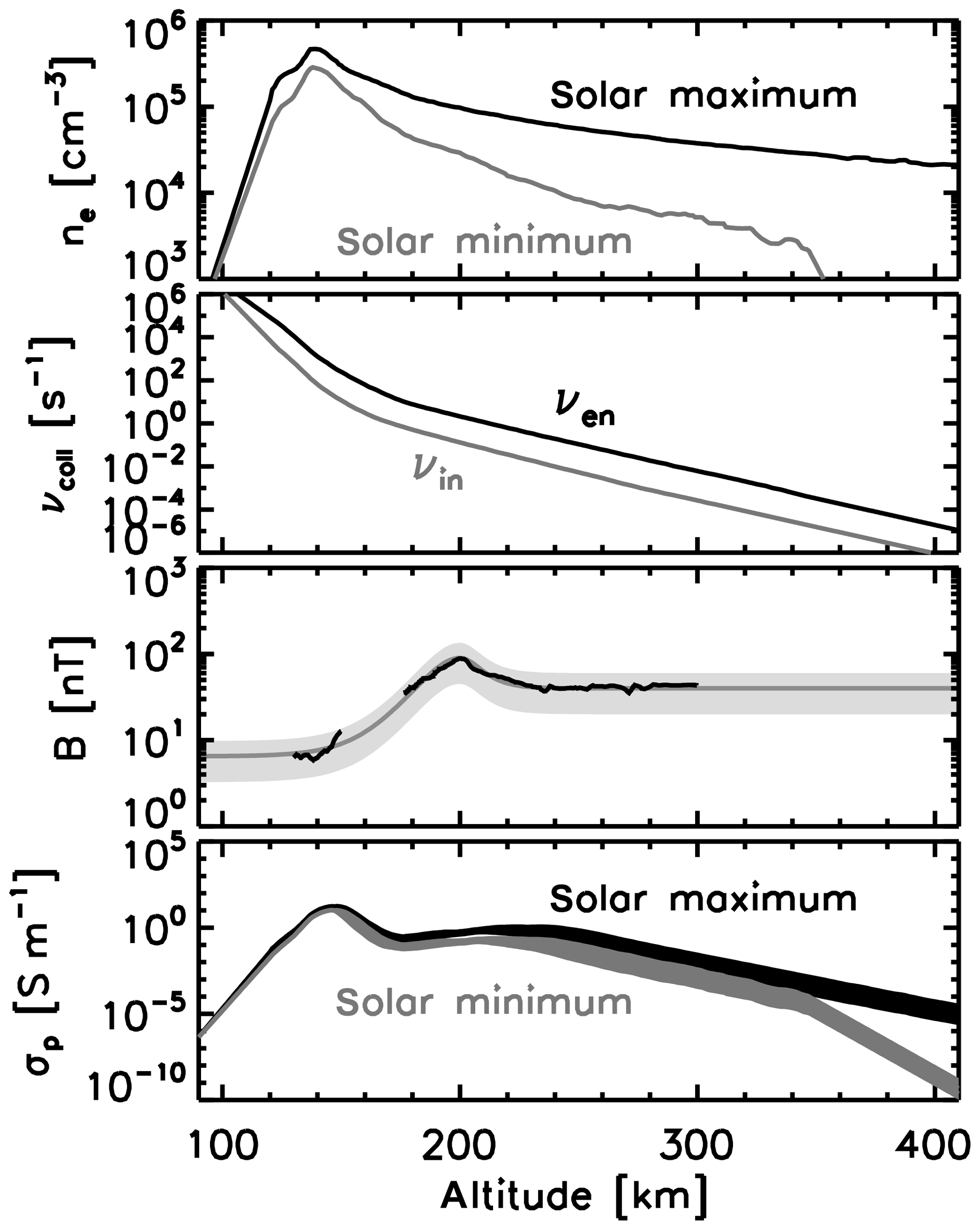
Figure 1Electron number density ne from Pioneer Venus Orbiter radio occultation measurement after Kilore and Luhmann (1991), model collision frequency between electrons and neutral particles νen and that between ions and neutral particles νin after Dubinin et al. (2014), magnetic field B after Venus Express measurements in black (after Villarreal et al., 2015 and Zhang et al., 2016) and model magnetic field with a fluctuation range (in gray), and Pedersen conductivity σp as a function of altitude from Venus' surface.
The task is to evaluate the electric conductivity as a function of the altitude. Since we work on the Pedersen conductivity for the magnetic diffusion problem, the electron density, the collision frequency, and the magnetic field profiles are needed to calculate the conductivity before performing the height integration. The procedure of the diffusion time estimate is summarized as follows.
-
Electron density profile. Altitude-dependent electron number density data are obtained by the Pioneer Venus Orbiter radio occultation measurements. We take values from Fig. 2 in Kilore and Luhmann (1991) at higher solar zenith angles (above 55∘), under the condition of solar maximum and that of solar minimum. The profile of the electron density is displayed in the first panel of Fig. 1.
-
Collision frequency profile. The profile of the collision frequency is taken from the recent calculation by Dubinin et al. (2014) (Fig. 16 in the article), which is based on theoretical velocity-moment estimates (Schunk and Nagy, 2000) using the temperature and neutral density profiles from Fox and Sung (2001). We consider the electron-neutral collisions and the ion-neutral collisions in the present work. The collision frequency is displayed as a function of the altitude in the second panel of Fig. 1.
-
Magnetic field profile. Magnetic field data from Venus Express are used as a reference from 300 to 180 km (Villarreal et al., 2015) and further down to 130 km (Zhang et al., 2016). The former data set is from a single event, but is illustrative in the model construction in that the transition is smooth with a magnetic pileup and an asymptotic behavior at higher altitudes (solid curve in black above an altitude of 170 km in the third panel of Fig. 1). The latter data set is from 33 periapsis passages, and we take the median values (solid curve in black below 150 km in the same panel). We use the secant function to construct a magnetic field model. The secant function is used separately below the magnetic pileup peak (set to z0=200 km altitude) and above the peak in the form of . We use the secant function as an empirical model because the secant function is known to describe solitary structures such as the KdV soliton (Korteweg–de Vries) or the density profile of the Harris current sheet. We obtain from the fitting procedure the following coefficients: (1) B0=40.0 nT (offset value), B1=50.0 nT (height of the secant bell shape), and d=7.0 km (width of the bell shape) for z0≥200 km, and (2) B0=6.5 nT, B1=83.5 nT, and d=12.0 km for z0≤200 km. The uncertainty of the magnetic field model is inferred from the statistical fluctuations shown in Zhang et al. (2016) and is approximated to a factor of 0.5 for the lower limit and a factor of 1.5 for the upper limit. Graphics of the magnetic field model are displayed in the third panel of Fig. 1.
-
Pedersen conductivity. We take the Pedersen conductivity (Dubinin et al., 2014; Vasyliūnas, 2012):
where ne is the electron number density, e the elementary charge, mi and me the mass of ions (assuming protons) and electrons, respectively, fgi and fge the gyrofrequency of ions and electrons (in units of s−1, not the angular frequency in units of rad s−1), νin the collision frequency between ions and neutrals, and νen the collision frequency between electrons and neutrals.
The ion term in the Pedersen conductivity (Eq. 4) should not be neglected because the ratio of the collision frequency to the respective (electron or ion) gyrofrequency is not negligible for the electrons and the ions. For example, Dubinin et al. (2014) show that the ion-neutral collision frequency exceeds the ion gyrofrequency at altitudes below 220 km. In contrast, the electron-neutral collision frequency exceeds the electron gyrofrequency at altitudes below 140 km. We evaluate the conductivity by keeping the ion term in Eq. (4) in the calculation. The dominant ion species are not protons but heavier species such as oxygen atoms O+ or molecules (Fox and Sung, 2001). We choose for the following mean ion masses: 11.6 proton mass or 23.3 proton mass, values taken from Dubinin et al. (2014). The Pedersen conductivity is displayed as a function of the altitude in the fourth panel of Fig. 1 for the solar maximum and minimum, respectively, including both the magnetic field models (high-field, mean-field and low-field) and the ion mass models. The peak conductivity is in the range at about 10 S m−1.
-
Integration. Height integration is performed to evaluate the diffusion time τd using Eq. (2) and the five-point Newton–Cotes integration formula. We resample values of the electron density, the collision frequency, and the model magnetic field for the numerical integration at a spatial resolution of 1 km and extrapolate the values in a linear fashion on the logarithmic scale at altitudes down to 100 km and up to 400 km. Most of the conductance (height-integrated conductivity) is confined around the maximum at 150 km. The contribution of this current-carrying layer from 140 to 170 km in altitude is around 78 %–85 % during the solar maximum (the variation comes from the choice of the magnetic field mode and the ion profile) and 88 %–91 % during the solar minimum.
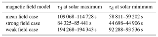
Table 1Results from the diffusion time estimate. The symbol τd stands for the diffusion time. The range in the table represents the choice for the mean ion mass (11.6 proton mass or 23.3 proton mass, values taken from Dubinin et al., 2014).
2.3 Results of diffusion time estimate
Diffusion time varies in the range from about 44 000 s (about 12 h) to about 194 000 s (54 h). See Table 1. Solar activity and the local magnetic field in the ionosphere influence the diffusion time. A minimum of 12 h (half a day) for the diffusion time is needed for the magnetic field to penetrate Venus' ionosphere and atmosphere. If the electron density is higher or the local magnetic field weaker, the diffusion time can scale up to 54 h (more than 2 days). Therefore, Venus' surface may exhibit a nonzero magnetic field when the solar wind is stationary (in the sense that the interplanetary magnetic field does not show a reversal) on the timescale of half a day to several days. For reference, we repeat the calculation of the diffusion time using only the electron term in the conductivity. The diffusion time from the electron term is in the range from about 40 000 s (11 h) to about 146 000 s (40 h). The ion contribution makes a difference in the diffusion time by about 10 %–20 %. Note that the peak Pedersen conductivity is about 14 S m−1 from the electron term and about 0.035 S m−1 (Table 2 right column), i.e., the ion contribution is only about 0.1 % at the peak of the Pedersen conductivity height profile.
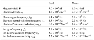
Table 2Comparison of Pedersen conductivity estimate at the peak altitudes of the conductivity; z=130 km on Earth and z=150 km on Venus. Electron density value on Earth is taken from Kelly (1989) at z=130 km. Electron density value on Venus is from Kilore and Luhmann (1991) during the solar maximum at an altitude of z=150 km (at the peak of Pedersen conductivity). Electron gyrofrequency is calculated from the nominal magnetic field magnitude. Collision frequency values on Earth are from Kertz (1989) and those on Venus are from Dubinin et al. (2014). A mean mass ratio of 11.6 is used between the ions and the protons.
3.1 Comparison with the hybrid simulations
It is interesting to observe the difference between the simulation and analytic estimates of the diffusion time by about 2 orders of magnitude. The major reason behind this difference most likely lies in the neglect of the electron-neutral collisions and the numerical diffusion in the hybrid simulations.
-
Electron contribution. The ion term in the conductance estimate contributes to a longer diffusion time by 10 %–20 %. In other words, the electron contribution to the conductance (and diffusion time) is somewhat 80 %–90 %, i.e., by neglecting this contribution the diffusion time is 5 to 10 times shorter than its actual value. Therefore, considering the electron contribution would increase the simulation proxy of 1000 to 5000–10000 s, i.e., 1.5–3 h. This reduces the difference between the simulation and analytic result by 1 order of magnitude.
-
Numerical diffusion. Problem of numerical oscillation, rounding or cutoff error, and numerical instabilities in the computation are suppressed either by adding an artificial diffusion or imposing a spatial smoothing (Bagdonat, 2002; Winske and Omidi, 1993). Here we estimate the diffusion coefficient or the conductivity for the smoothing procedure. First, we rewrite the magnetic diffusion equation
into the time-advancing formula as
where η denotes the diffusion coefficient of the magnetic field, B is the magnetic field, Δt is the time step in the simulation, and ℓ is the length scale of the gradient. Second, in the smoothing method, the magnetic field is smoothed by the following procedure (Bagdonat, 2002; Müller et al., 2011; Winske and Omidi, 1993):
where αsm is a free parameter called the smoothing factor (its value of αs is typically 0.01 to 0.1) and 〈B〉 is the locally smoothed magnetic field. Now, by comparing the right-hand side of Eq. (6) with the smoothing term αsmB in Eq. (8), we obtain a relation between the smoothing factor αsm and the diffusion coefficient η as follows:
Using the relation to the conductivity , Eq. (9) is expressed as
We evaluate Eq. (10) using the following values: the smoothing parameter αsm=0.01 (i.e., 1 % spatial smoothing) from Müller et al. (2011), ℓ=100 km (grid size in the simulation) from Bößwetter et al. (2004) and Martinecz et al. (2009), Δt=1 s (typical ion gyroperiod in the solar wind), and H m−1 (permeability of free space). We also obtain the numerical conductivity (or the smoothing conductivity) S m−1. Hence, the numerical conductivity equivalent to the spatial smoothing procedure for the purpose of numerical damping in the hybrid simulation is of the order of 10−2 S m−1. The physical conductivity from our study is 1–10 S m−1 at the peak.
The magnetic diffusion time is L2μ0σ and the diffusion length scale L is the same as the grid scale l. Hence, the diffusion time is proportional to the conductivity in our problem, and the difference in the diffusion time by 2 orders of magnitude between the hybrid simulations (about 1000 s) and our semi-analytic estimate (about 100 000 s) can reasonably be explained by the spatial smoothing procedure in the simulation.
3.2 Comparison with Earth's ionosphere
It is also interesting to observe that the Pedersen conductivity on Venus is much higher than on Earth by about 4 orders of magnitude. This difference can be explained as follows. We write formulas separately for the electron Pedersen conductivity σp,e S m−1 as
and the ion Pedersen conductivity σp,i S m−1 as
where a mass ratio of or is used (mi is the ion mass, mp is the proton mass, and me is the electron mass).
The Pedersen conductivity on Venus is primarily contributed by the electron-neutral collisions. By ignoring the gyrofrequency, Venus' Pedersen conductivity is approximately as follows.
The Pedersen conductivity on Earth is, in contrast to the Venus case, contributed by the ion-neutral collisions.
The reason for this is that the gyrofrequency exceeds the electron-neutral collision frequency at an altitude of 60–70 km and above due to a stronger magnetic field (than that of Venus). Now we compare Eq. (15) with Eq. (16).
Using the facts that (1) the electron density is almost the same (ne∼105 cm−3) between Venus (peak altitude z=150 km) and Earth (peak altitude z=130 km), (2) the typical mass ratio from the ions to the electrons is about 20 000 (about 11 proton mass), and (3) the collision frequency is roughly of the same order between Venus and Earth, Hz and Hz on Earth, respectively, we obtain the ratio of the peak Pedersen conductivity from Venus to Earth as follows:
The difference in the peak Pedersen conductivity by nearly four orders of magnitude can essentially represent the difference in the Pedersen current carrier in the different magnetic field environments: the Pedersen current is carried by the electrons on Venus and by the ions on Earth. More detailed calculations of the peak Pedersen conductivity on Earth and Venus are shown in Table 2.
We conclude the diffusion time estimate with the following notes. First, a stationary solar wind condition on a timescale of half a day to several days is likely occurring in Venus' environment. The interplanetary magnetic field can theoretically reach (under the condition of stationary solar wind) Venus' surface and justifies the nonzero field measurements by Venus Express. Second, further improvement is possible by including the ion-neutral collisions and the solar activity influence on the collision frequency. Third, the upcoming missions such as Parker Solar Probe (Fox et al., 2016), BepiColombo (Benkhoff et al., 2010), and Solar Orbiter (Müller et al., 2013) will perform magnetic field and plasma measurements in the near-Venus environment for a variety of distances and approaching directions to Venus. For example, two Venus flyby manoeuvres are planned for BepiColombo: Flyby 1 in October 2020 down to 11 317 km, and Flyby 2 in August 2021 down to 1000 km. Even though BepiColombo's flybys at Venus are too far to directly measure the near-surface magnetic field, the flyby data will help us to determine or constrain the stability of IMF and the condition for the magnetic field penetration through the ionosphere for several hours to a day. The direct test for the magnetic field penetration would ideally be performed during a stable IMF period, for another Venus mission in future.
Input data used in this work are graphically available in the articles by Kilore and Luhmann (1991) for the electron number density, Dubinin et al. (2014) for the collision frequency, and Villarreal et al. (2015) and Zhang et al. (2016) for the magnetic field.
YN carried out the calculation, writing, and revision work. UM came up with the original idea and handled the discussion and finalization.
The authors declare that they have no conflict of interest.
The authors thank those at the Europlanet workshop
Planetary Atmospheric Erosion
in Murighiol, Romania, 11–15 June 2018,
hosted by Institute for Space Sciences in Bucharest-Măgurele, for stimulating and fruitful
discussion.
Yasuhito Narita thanks Daniel Heyner for the information about
the BepiColombo Venus flyby plan.
Edited by: Elias Roussos
Reviewed by: Octav
Marghitu
Bagdonat, T. B.: Hybrid simulations of weak comets, PhD thesis, Tech. Univ. Braunschweig, Braunschweig, 2002. a, b
Benkhoff, J., van Casteren, J., Hayakawa, H., Fujimoto, M., Laakso, H., Novara, M., Ferri, P., Middleton, H. R., and Ziethe, R.: BepiColombo – Comprehensive exploration of Mercury: Mission overview and science goals, Planet. Space Sci., 58, 2–20, https://doi.org/10.1016/j.pss.2009.09.020, 2010. a
Bößwetter, A.: Wechselwirkung des Mars mit dem Sonnenwind: Hybrid-Simulationen mit besonderem Bezug zur Wasserbilanz, PhD thesis, Tech. Univ. Braunschweig, Braunschweig, Germany, https://publikationsserver.tu-braunschweig.de/receive/dbbs_mods_00028707 (last access: 15 November 2018), 2009. a
Bößwetter, A., Bagdonat, T., Motschmann, U., and Sauer, K.: Plasma boundaries at Mars: a 3-D simulation study, Ann. Geophys., 22, 4363–4379, https://doi.org/10.5194/angeo-22-4363-2004, 2004. a, b
Dimmock, A. P., Alho, M., Kalio, E., Pope, S. A., Zhang, T. L., Kilpua, E., Pulkkinen, T. I., Futaana, Y., and Coates, A. J.: The response of the Venusian plasma environment to the passage of an iCME: Hybrid simulation results and Venus Express observations, J. Geophys. Res.-Space, 123, 3580–3601, https://doi.org/10.1029/2017JA024852, 2018. a
Dubinin, E., Fraenz, M., Zhang, T. L., Woch, J., and Wei, Y.: Magnetic fields in the Venus ionosphere: Dependence on the IMF direction: Venus express observations, J. Geophys. Res.-Space, 119, 7587–7600, https://doi.org/10.1002/2014JA020195, 2014. a, b, c, d, e, f, g
Fox, J. L. and Sung, K. Y.: Solar activity variations of the Venus thermosphere/ionosphere, J. Geophys. Res., 106, 21305–21335, https://doi.org/10.1029/2001JA000069, 2001. a, b
Fox, N. J., Velli, M. C., Bale, S. D., Decker, R., Driesman, A., Howard, R. A., Kasper, J. C., Kinnison, J., Kusterer, M., Lario, D., Lockwood, M. K., McComas, D. J., Raouafi, N. E., and Szabo, A.: The Solar Probe Plus Mission: Humanity's first visit to our star, Space Sci. Rev., 204, 7–48, https://doi.org/10.1007/s11214-015-0211-6, 2016. a
Kelly, M. C.: The Earth’s Ionosphere, Academic Press, Inc., San Diego, 1989. a
Kertz, W.: Einführung in die Geophysik II, BI Hochschultaschenbücher, 1989. a
Kliore, A. J. and Luhmann, J. G.: Solar cycle effects on the structure of the electron density profiles in the dayside ionosphere of Venus, J. Geophys. Res., 96, 21281–21289, 1991. a, b, c
Martinecz, C.: The Venus plasma environment: a comparison of Venus Express ASPERA-4 measurements with 3D hybrid simulations, PhD thesis, Tech. Univ. Braunschweig, Braunschweig, Germany, https://publikationsserver.tu-braunschweig.de/receive/dbbs_mods_00024412 (last access: 15 November 2018), 2008. a
Martinecz, C., Boesswetter, A., Fränz, M., Roussos, E., Woch, J., Krupp, N., Dubinin, E., Motschmann, U., Wiehle, S., Simon, S., Barabash, S., Lundin, R., Zhang, T. L., Lammer, H., Lichtenegger, H., and Kulikov, Y.: Plasma environment of Venus: Comparison of Venus Express ASPERA-4 measurements with 3-D hybrid simulations, J. Geophys. Res., 114, E00B30, https://doi.org/10.1029/2008JE003174, 2009, Correction in 114, E00B98, https://doi.org/10.1029/2009JE003377, 2009. a, b
Müller, D., Marsden, R. G., St. Cyr, O. C., and Gilbert, H. R.: Solar Orbiter: Exploring the Sun-Heliosphere Connection, Solar Phys., 285, 25–70, https://doi.org/10.1007/s11207-012-0085-7, 2013. a
Müller, J., Simon, S., Motschmann, U., Schüle, J., Glassmeier, K.-H., and Pringle, G. J.: A.I.K.E.F.: Adaptive hybrid model for space plasma simulations, Comp. Phys. Comm., 182, 946–966, https://10.1016/j.cpc.2010.12.033, 2011. a, b
Russell, C. T., Chou, E., Luhmann, J. G., Gazis, P., Brace, L. H., and Hoegy, W. R.: Solar and interplanetary control of the location of the Venus bow shock, J. Geophys. Res., 93, 5461–5469, https://doi.org/10.1029/JA093iA06p05461, 1988. a
Russell, C. T., Strangeway, R. J., Luhmann, J. G., and Brace, L. H.: The magnetic state of the lower ionosphere during Pioneer Venus entry phase, Geophys. Res. Lett., 20, 2723–2726, https://doi.org/10.1029/93GL02625, 1993. a
Saunders, M. A. and Russell, C. T.: Average dimension and magnetic structure of the distant Venus magnetotail, J. Geophys. Res., 91, 5589–5604, https://doi.org/10.1029/JA091iA05p05589, 1986. a
Schunk, R., and Nagy, A.: Ionospheres: Physics, Plasma Physics and Chemistry, Cambridge Atmos. Space Sci. Ser., 88, 96–99, Cambridge Univ. Press, Cambridge, U. K., and New York, 2000. a
Vasyliūnas, V. M.: The physical basis of ionospheric electrodynamics, Ann. Geophys., 30, 357–369, https://doi.org/10.5194/angeo-30-357-2012, 2012. a
Villarreal, M. N., Russell, C. T., Wei, H. Y., Ma, Y. J., Luhmann, J. G., Strangeway, R. J., and Zhang, T. L.: Characterizing the low-altitude magnetic belt at Venus: Complementary observations from the Pioneer Venus Orbiter and Venus Express, J. Geophys. Res., 120, 2232–2240, https://doi.org/10.1002/2014JA020853, 2015. a, b
Winske, D. and Omidi, N.: Hybrid codes: Methods and applications, Terra Publication, Tokyo, 1993. a, b
Zhang, T. L., Baumjohann, W., Delva, M., Auster, H.-U., Balogh, A., Russell, C. T., Barabash, S., Balikhin, M., Berghofer, G., Biernat, H. K., Lammer, H., Lichtenegger, H., Magnes, W., Nakamura, R., Penz, T., Schwingenschuh, K., Vörös, Z., Zambelli, W., Fornacon, K.-H., Glassmeier, K.-H., Richter, I., Carr, C., Kudela, K., Shi, J. K., Zhao, H., Motschmann, U., and Lebreton, J.-P.: Magnetic field investigation of the Venus plasma environment: Expected new results from Venus Express, Planet. Space Sci., 54, 1336–1343, https://doi.org/10.1016/j.pss.2006.04.018, 2006. a
Zhang, T. L., Baumjohann, W., Russell, C. T., Villarreal, M. N., Luhmann, J. G., and Teh, W. L.: A statistical study of the low-altitude ionospheric magnetic fields over the north pole of Venus, J. Geophys. Res.-Space, 120, 6218–6299, https://doi.org/10.1002/2015JA021153, 2015. a
Zhang, T. L., Baumjohann, W., Russell, C. T., Luhmann, J. G., and Xiao, S. D.: Weak, quiet magnetic fields seen in the Venus atmosphere, Nature Sci. Rep., 6, 23537, https://doi.org/10.1038/srep23537, 2016. a, b, c, d