Electromagnetic field observations by the DEMETER satellite in connection with the 2009 L'Aquila earthquake

To define a background in the electromagnetic emissions above seismic regions, it is necessary to define the statistical distribution of the wave energy in the absence of seismic activity and any other anomalous input (e.g. solar forcing). This paper presents a completely new method to determine both the environmental and instrumental backgrounds applied to the entire DEMETER satellite electric and magnetic field data over L'Aquila. Our technique is based on a new data analysis tool called ALIF (adaptive local iterative filtering, Cicone et al., 2016; Cicone and Zhou, 2017; Piersanti et al., 2017b). To evaluate the instrumental background, we performed a multiscale statistical analysis in which the instantaneous relative energy (ϵ_rel), kurtosis, and Shannon entropy were calculated. To estimate the environmental background, a map, divided into ${\mathrm{1}}^{\circ }\times {\mathrm{1}}^{\circ }$ latitude–longitude cells, of the averaged relative energy ($\stackrel{\mathrm{‾}}{{\mathit{ϵ}}_{\mathrm{rel}}}$), has been constructed, taking into account the geomagnetic activity conditions, the presence of seismic activity, and the local time sector of the satellite orbit. Any distinct signal different (over a certain threshold) from both the instrumental and environmental backgrounds will be considered as a case event to be investigated. Interestingly, on 4 April 2009, when DEMETER flew exactly over L'Aquila at UT = 20:29, an anomalous signal was observed at 333 Hz on both the electric and magnetic field data, whose characteristics seem to be related to pre-seismic activity.

1 Introduction

The nature of the Earth's interior, in terms of the dynamics of the crust, mantle, and core, can be investigated through extended ground-based and space observations (Bell, 1982; Hayakawa and Molchanov, 2002; Pulinets and Boyarchuk, 2004; De Santis et al., 2015). In the same way, it is possible to inquest the natural or anthropogenic origin of the electromagnetic emissions (EMEs) using measurements in the near-Earth space (Parrot and Zaslavski, 1996; Buzzi, 2006). In addition, several works (Parrot, 1995; Parrot and Zaslavski, 1996; Buzzi, 2007) remarked that EMEs of both anthropogenic (such as HF broadcasting stations and VLF transmitters) and natural (i.e. Earth's surface) origin can influence the dynamics and the composition of the ionosphere–magnetosphere region (Parrot and Molchanov, 1995; Parrot and Zaslavski, 1996). Taking into account that extreme reliability is needed to call for preseismic phenomena, a characteristic background for the regions on Earth where we want to detect the effects of earthquake-related EMEs should be available. In the interim, comprehensive study of both magnetospheric and ionospheric disturbances driven by ground preseismic EME waves has to be carried out. In this context, aseismic fault creep and EME waves are expected to be the principal mechanical and electromagnetic earthquake precursors, respectively (Buzzi, 2007, and references therein). Parrot and Molchanov (1995) and Parrot and Zaslavski (1996) achieved the first promising result analysing rare EME wave observations over the ionosphere–magnetosphere region. In their studies, they first distinguished between internal and external components of the geomagnetic field and, then, gave an efficient measure of the electric field, the plasma temperature, and the density of the ionosphere. Despite several theoretical models having been developed, the physical mechanisms leading to the observation of these effects both at ground and in space are as yet largely unexplained. That is, the following remains to be understood: the genesis of EME waves over the focal area (especially soon before a seismic event, if any); its propagation through lithospheric layers characterized by fixed vertical conductivity; its access into both the neutral atmosphere and ionosphere; and its arrival in the magnetosphere and its relative interaction. It is worth noting that, when a EME wave propagates through both the ionosphere and magnetosphere, the medium has to be considered dispersive too (Chen, 1977). Recently, Perrone et al. (2018) analysed ionosonde data and crustal earthquakes with magnitude M≥6.0 observed in Greece during 2003–2015 to check whether the relationships obtained between precursory ionospheric anomalies and earthquakes in Japan and central Italy are also valid for Greek earthquakes. They identified the ionospheric anomalies as observed variations of the sporadic E-layer parameters (h^′Es, foEs) and foF2 at the ionospheric station of Athens and found similar corresponding empirical relationships between the seismoionospheric disturbances and the earthquake magnitude and the epicentral distance. Moreover, the large lead times found for the ionospheric anomalies' occurrence seem to confirm a rather long earthquake preparation period.

The search for ionospheric disturbances associated with earthquakes relies on thorough statistical studies to disentangle seismic effects from the variations induced by the physical processes that control the ionosphere dynamic and natural emissions. Several studies have been performed, in the framework of the DEMETER (Detection of Electro-Magnetic Emissions Transmitted from Earthquake Regions) mission, and one of them has shown a decrease in the extremely low-frequency (ELF) wave intensity in the frequency range between 1 and 2 kHz a few hours before the shock (Parrot et al., 2006; Píša et al., 2012 and 2013; Zhang et al., 2012; Walker et al., 2013). Nĕmec et al. (2008) built a statistical map of electromagnetic wave intensity obtained from DEMETER satellite ICE and IMSC data available at that time (2004–2007). Then, they estimated the probability of occurrence during a seismic event of signals with higher intensity with respect to the background level defined by the map. Their study was the first attempt to generate a background map in the electromagnetic emission above seismic regions for the determination of the statistical distribution of the wave energy in the absence of seismic activity.

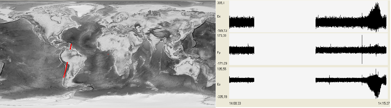
Figure 1 Typical ELF data of a half-orbit (orbit no. 302630 on 2010/02/26 day-side). It is shown that data are not available along the whole orbit, but only when the satellite was in “burst mode”.

The present paper uses a completely new method to determine both the environmental and instrumental backgrounds in the electromagnetic emission above seismic regions by using the DEMETER satellite electric and magnetic field observations. This algorithm is based on a new data analysis technique called ALIF (adaptive local iterative filtering, Cicone et al., 2016, 2017; Piersanti et al., 2017b) and through a multiscale statistical analysis of the electromagnetic observations. The results obtained with this technique allowed the construction of an electromagnetic energy background map over the L'Aquila seismic region from 2004 to 2011. In addition, on 4 April 2009, 2 days before the 6.3 M_w earthquake (USGS Earthquake catalogue), when DEMETER flew exactly over L'Aquila at UT = 20:29, an anomalous signal with respect to the background was observed.

2 Data and methods

2.1 DEMETER data

In our study, we used the data from French satellite DEMETER, launched in 2004 on a Sun-synchronous orbit at about 700 km in altitude. The orbits of the satellite had an inclination of 98^∘ and a local time of 10:30 on the day-side and 22:30 on the night-side. The instruments were operational at geomagnetic latitudes between −65 and +65^∘, thus providing a good coverage of the Earth's seismic zones (Parrot et al., 2005). The data from the ICE electric field experiment (Berthelier et al., 2005) and the IMSC magnetic field experiment (Parrot et al., 2005) were used in order to detect any electromagnetic waves. Among the four available DEMETER channels we selected the ELF band, the only one which provides the wave form of the three components of the fields. The ELF specification is a data range in the frequency from 15 Hz to 1 kHz, with a sample rate of 2.5 kHz. Due to the high data transfer resources required, the ELF acquisition is operational only in “burst mode”, so data are available only in a fraction of the entire orbit (see Fig. 1). The DEMETER mission lasted from 2004 to March 2011, so we have a large dataset of almost 7 years of the satellite observations, altogether representing 71 730 half-orbits (35 865 on the day-side and 35 865 on the night-side). Within the entire available dataset, we selected the orbits with ELF data that covered a squared area of ${\mathrm{1}}^{\circ }\times {\mathrm{1}}^{\circ }$ (latitude and longitude) centred over L'Aquila's geographic coordinates.

2.2 ALIF

The algorithm for the evaluation of both environmental and instrumental backgrounds in the electromagnetic emission above seismic regions is based on a recent data analysis technique called ALIF, developed by Cicone et al. (2016) and Piersanti et al. (2017b). ALIF is able, through a time-frequency analysis, to identify and quantify the variations across different scales for non-stationary signals due to the complexity and non-linearity of the system that generated them. The reason for using this technique is that, unlike typical data analysis methods, such as fast Fourier transform and wavelet, ALIF does not suffer from either limited resolution (Cohen, 2001) and interferences in the time-frequency domain (Flandrin, 1998). Thus, ALIF does not require any further processing of the representation. The key idea behind this method, very similar to the empirical mode decomposition (EMD, Huang et al., 1998), is a “divide et impera” approach. In fact, ALIF first decomposes a signal into several functions oscillating around zero and characterized by frequencies variable with time (intrinsic mode functions – IMFs). Then, for each IMF, it performs a time analysis. The great difference with EMD is that ALIF has a strong mathematical structure which guarantees the convergence and stability of the algorithm, which in turn guarantees the physical significance of the decomposition (Piersanti et al., 2017b).

2.3 Multiscale statistical analysis and standardized mean (SM) test

In order to evaluate the instrumental and environmental background of a signal s(t) (such as the magnetic and electric field observations), we study its multiscale properties. To accomplish this task, we first use ALIF to decompose s(t) into functions IMF_ℓ(t), characterized by a peculiar scale of variability ℓ (Wernik, 1997), so that

$$s\left(t\right)=\sum _{\mathrm{\ell }=\mathrm{1}}^m{\mathrm{IMF}}_{\mathrm{\ell }}\left(t\right)+r\left(t\right),$$

where r(t) is the residue of the decomposition. The connection between each IMF and the scale of variability ℓ of s(t) has been analyzed by using the Flandrin (1998) technique: a dataset characterized by an evident scale separation can be decomposed into two contributions:

$$s\left(t\right)=s_{\mathrm{0}}\left(t\right)+\mathit{\delta }s\left(t\right),$$

where s₀(t) is named the baseline and δs(t) represents the variations around the baseline. To identify δs(t), we applied the method proposed by Alberti et al. (2016), by defining δs(t) as the reconstruction of a subset s₁ of k<m modes,

$$\begin{array}{}\text{(1)}& \mathit{\delta }s\left(t\right)={\sum }_{\mathrm{\ell }=\mathrm{1}}^k{\mathrm{IMF}}_{\mathrm{\ell }}\left(t\right),\end{array}$$

characterized by a standardized mean (i.e. the mean divided by the standard deviation) SM ≈ 0 and by IMF fluctuating at higher frequency.

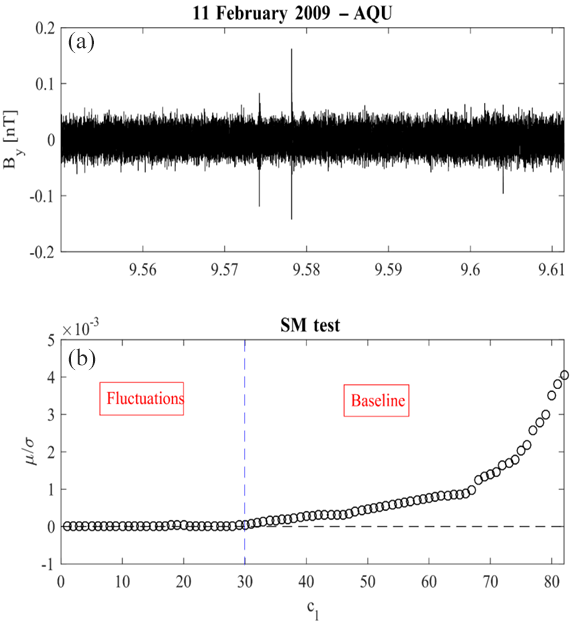
Figure 2 An example of the application of the SM test (b) to the magnetic field observations (a) over l'Aquila on 11 February 2009 from 09:33 to 09:39 UT.

Figure 2 shows an example of the application of the SM test to the DEMETER magnetic field observations (upper panel) over L'Aquila ($\mathit{\lambda }={\mathrm{42.334}}^{\circ }$, $\mathit{\phi }={\mathrm{13.334}}^{\circ }$; LT = UT+1) on 11 February 2009 from 09:33 to 09:37 UT. The lower panel shows the SM test results. It can be easily seen that IMFs from 1 to 30 represent the fluctuating part of the signal (δB_y), while IMFs from 31 to 82 are the baseline ($B_{y_{\mathrm{0}}}$). To distinguish between instrumental origin fluctuations and real signals, a multiscale statistical analysis is needed. For the different scales ℓs, we considered the statistics of the values IMF_ℓ(t). This technique, called multiscale statistical analysis, calculates and studies the second (the variance σ(ℓ)), third (the skewness Sk(ℓ)), and fourth (the kurtosis excess $K_{\mathrm{ex}}\left(\mathrm{\ell }\right)=K\left(\mathrm{\ell }\right)-\mathrm{3}$) moments of the probability distribution p(IMF_ℓ(t)) of IMF_ℓ(t), the relative energy ϵ_rel, and the Shannon information entropy I(ℓ), respectively defined as

$$\begin{array}{}\text{(2)}& {\displaystyle }& {\displaystyle }{\mathit{ϵ}}_{\mathrm{rel}}\left(\mathrm{\ell }\right)={\displaystyle \frac{{\int }_{\mathrm{\ell }}\mathrm{|}{\mathrm{IMF}}_{\mathrm{\ell }}\left(t\right){\mathrm{|}}^{\mathrm{2}}\mathrm{d}t}{{\int }_{\mathrm{\ell }}\mathrm{|}s\left(t\right){\mathrm{|}}^{\mathrm{2}}\mathrm{d}t}},\text{(3)}& {\displaystyle }& {\displaystyle }\mathrm{I}\left(\mathrm{\ell }\right)=-{\sum }_{\left\{{\mathrm{IMF}}_{\mathrm{\ell }}\right\}}p\left({\mathrm{IMF}}_{\mathrm{\ell }}\left(\mathrm{t}\right)\right)\cdot {\log }_{\mathrm{2}}\mathrm{p}\left({\mathrm{IMF}}_{\mathrm{\ell }}\left(\mathrm{t}\right)\right).\end{array}$$

These parameters measure the variability of the statistics of the signal in the function of the scale considered (Strumik and Macek, 2008). That is, K_ex(ℓ) indicates how the different ℓs are rich in rare fluctuations (Frisch, 1995); ϵ_rel measures how “energetically strong” the ℓ component is in Eq. (1). I(ℓ) measures the “degree of randomness” of each IMF_ℓ(t) component of the signal. In our case the scale ℓ corresponds to the peculiar frequency of each IMF of both magnetic and electric field observations.

2.4 Instrumental background

We define IMF_ℓ(t) as having an instrumental origin if two conditions are satisfied at the same time.

1. The SM test evaluates the IMF_ℓ(t) as a fluctuation;

2. K_ex (IMF_ℓ(t)) is almost null and correspondingly I(IMF_ℓ(t)) presents a relative maximum.

Indeed, an IMF_ℓ(t) that satisfies these two conditions can be represented as a Gaussian fluctuation characterized by a high “degree of randomness”. Thus, it can be identified as instrumental noise. Figure 3 shows an example of a multiscale statistical analysis of the B_y component of the DEMETER satellite for the same period of Fig. 2. Figure 3a shows the ϵ_rel behaviour as a function of the scale ℓ (i.e. the frequency). Two energy peaks, at 20 Hz (blue dashed line) and 333 Hz (green dashed line), are clearly visible. Scales lower than 3 Hz have almost null energy (red dashed line), have K_ex(ℓ)∼0, and show the highest values of I(ℓ). The IMFs corresponding to these scales could be attributed to instrumental noise. In any event, a more accurate analysis of each IMF in the interval ℓ<3 Hz will be done in the next sections. On the other hand, the IMFs related to 20 Hz are not of instrumental origin because, despite the almost null value of K_ex, the Shannon entropy proves to be concave-upward. In fact, ≅ℓ20 Hz is one of the peaks of Shumann resonance in the ELF portion of the Earth's electromagnetic field spectrum generated and excited by lightning discharges in the cavity formed by the Earth's surface and the ionosphere (Barr et al., 2000, and references therein). A similar situation is obtained for ℓ=333 Hz. In fact, the relative K_ex(ℓ)=3 (Fig. 3b) and I(ℓ) (Fig. 3c) prove to be concave-upward. Thus, the signal associated with 333 Hz does not originate from instrumental noise.

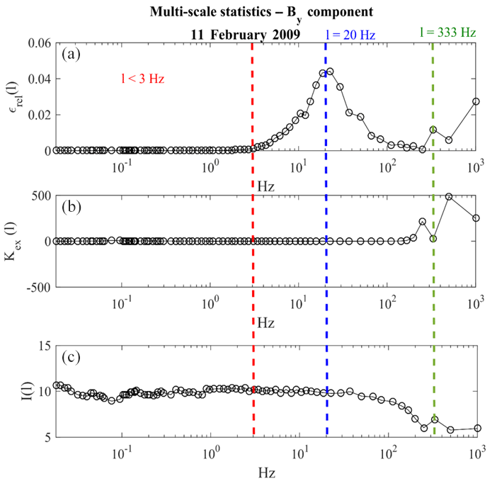
Figure 3 Example of a multiscale statistical analysis of the B_y component for the same data of Fig. 2: (a) ϵ_rel vs. frequency; panel (b) K_ex vs. frequency; panel (c) I vs. frequency. Two energy peaks, at 20 Hz and at 333 Hz are clearly visible.

By the use of those criteria, we can identify all the n<m IMFs(ℓ) originating from instrumental noise. As a consequence, the instrumental background can be defined as

$$R_b=\sum _{\mathrm{\ell }=\mathrm{1}}^n\mathrm{IMF}\left(\mathrm{\ell }\right),$$

where R_b is the signal of instrumental origin.

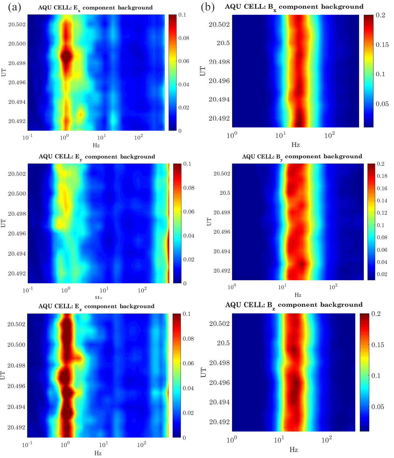
Figure 4 Environmental background for the L'Aquila cell as evaluated by ALIF in terms of $\stackrel{\mathrm{‾}}{{\mathit{ϵ}}_{\mathrm{rel}}}\left(\mathrm{\ell }\right)$ vs. time and frequency for the reference quiet period (M<3, Kp <2, L= night-side). (a) shows the $\stackrel{\mathrm{‾}}{{\mathit{ϵ}}_{\mathrm{rel}}}\left(\mathrm{\ell }\right)$ for the three components of the electric field; (b) shows the $\stackrel{\mathrm{‾}}{{\mathit{ϵ}}_{\mathrm{rel}}}\left(\mathrm{\ell }\right)$ for the three components of the magnetic field.

2.5 Environmental background

The environmental background has been evaluated through the following steps.

1. We divided the entire electric and magnetic DEMETER dataset into two subsets depending on the local time sector of the satellite orbit (i.e. day-side or night-side). Each subset has again been divided into two more subsets characterized by different seismic conditions. The first one (M_L) is defined for low seismic activity (M≤3, M being the earthquake magnitude) and the second (M_H) for high seismic activity (M>3). This procedure is crucial to take into account the nature of the earthquake and the different ionospheric response.

2. As in Perrone et al. (2018), all M_L and M_H subsets were again divided into three subsets according to the level of geomagnetic activity. This division is important to take into account possible signals associated with geomagnetic activity. To accomplish this task, we used either the Sym-H index or the AE index. The first one is the ring current activity index, which takes into account possible low-latitude geomagnetic activity (McPherron et al., 1986). The second is the auroral electrojet activity index, which takes into account possible high-latitude geomagnetic activity induced by the loading–unloading process from the magnetotail current (Akasofu, 2017). The three subsets correspond to three intervals, which are I_k,1: Sym-H = [10 nT, −10 nT) and AE < 100 nT; I_k,2: Sym-H = [−10 nT, −80 nT) and AE < 150 nT; and I_k,3: Sym-H ≤ −80 nT and AE ≥ 150 nT. I_k,1, I_k,2, and I_k,3 correspond to quiet, moderate, and high geomagnetic activity. Since both the Sym-H and AE indices have 1 min resolution, to assign each orbit to the correct “geomagnetic activity” interval, we considered their behaviour 24 h before the event under analysis.

   As a consequence, we finally obtained a total of 12 intervals (hereafter $C_{\mathrm{M},\mathrm{K},\mathrm{L}}$, where the subscripts M, K, and L correspond to the magnitude interval, geomagnetic activity interval, and local time interval of the satellite orbit, respectively).

3. The world map has been divided into ${\mathrm{1}}^{\circ }\times {\mathrm{1}}^{\circ }$ latitude–longitude cells. Each $C_{\mathrm{M},\mathrm{K},\mathrm{L}}$ will be decomposed by ALIF. For each cell, after the removal of instrumental noise by applying the technique described above, a time-frequency ϵ_rel will be calculated. Then, a mean $\stackrel{\mathrm{‾}}{{\mathit{ϵ}}_{\mathrm{rel}}}$ will be calculated and stored for each frequency scale. Averaging has been applied only if the ratio $R_{\mathit{ϵ}}\left(\mathrm{\ell }\right)=\frac{{\mathit{ϵ}}_{\mathrm{rel}}\left(\mathrm{\ell }\right)}{\stackrel{\mathrm{‾}}{{\mathit{ϵ}}_{\mathrm{rel}}}\left(\mathrm{\ell }\right)}=\mathrm{1}\pm \mathrm{3}\mathit{\sigma }\left(\mathrm{\ell }\right)$, where σ(ℓ) is the standard deviation of $\stackrel{\mathrm{‾}}{{\mathit{ϵ}}_{\mathrm{rel}}}$ evaluated at the single frequency scale ℓ.

For each $C_{\mathrm{M},\mathrm{K},\mathrm{L}}$, we defined $\stackrel{\mathrm{‾}}{{\mathit{ϵ}}_{\mathrm{rel}}}\left(\mathrm{\ell }\right)$ as the environmental background. This kind of background gives a representation of both the magnetospheric and ionospheric electric and magnetic field activity directly driven by the geoelectric and geomagnetic field variations induced by solar forcing. As a consequence, any distinct signal (over the threshold 1±3σ(ℓ)) could be reasonably studied as an anomalous event.

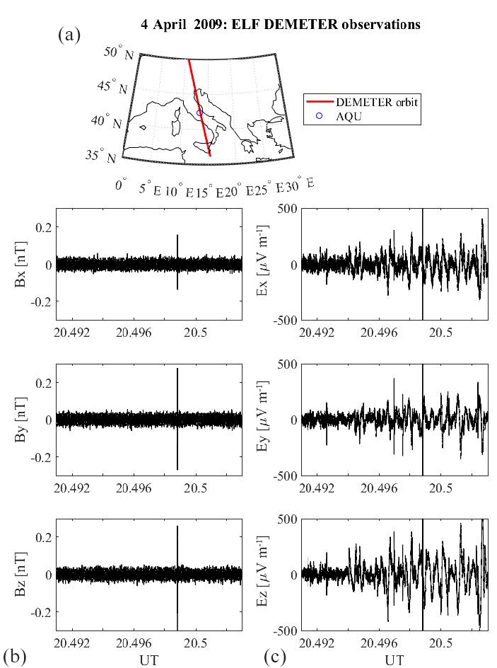
Figure 5 DEMETER electromagnetic observation on 4 April 2009 in the ELF band. (a) shows the satellite orbit (red) as a function of the geographic latitude and longitude. Lower panels show the electric (c) and magnetic (b) field observations as a function of the universal time (UT). The blue circle identifies the L'Aquila geographic position.

Figure 4 shows the background components of both the electric (left panels) and magnetic (right panels) fields over the L'Aquila cell ($C_{\mathrm{M},\mathrm{K},\mathrm{L}}$: 1^∘ in latitude and 1^∘ in longitude centred at the L'Aquila geographic coordinate) with M<3, −10 nT < Sym-H < 0 nT and AE < 100 nT, L = night-side, which we defined as being the quiet background condition. For the evaluation we used 72 satellite orbits. The results are presented in the satellite reference framework¹ (Berthelier et al., 2005).

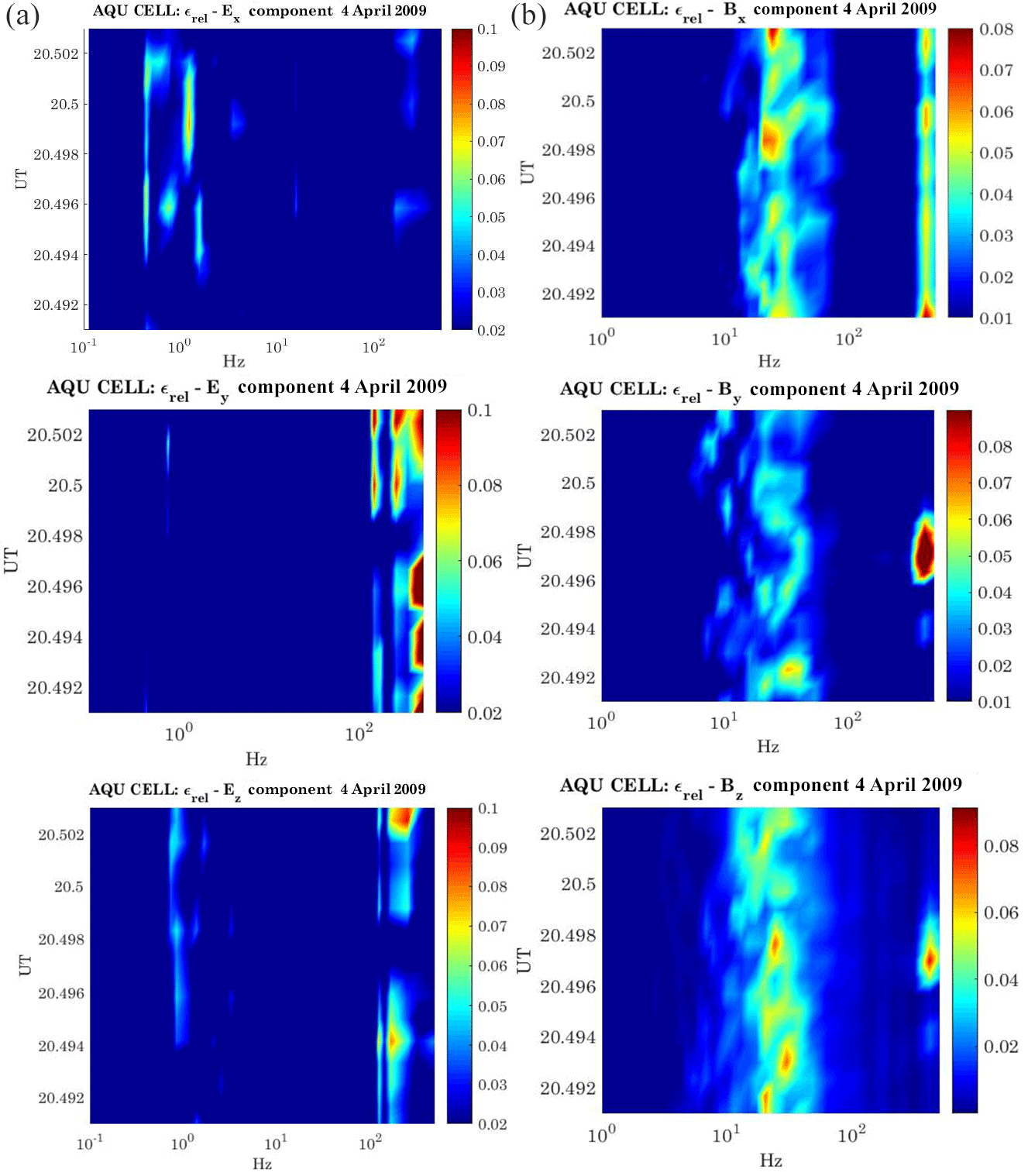
Figure 6 Anomalous event detected over L'Aquila on 4 April 2009. (a) shows the ϵ_rel(ℓ) vs. time and frequency for the three components of the electric field; (b) shows the ϵ_rel(ℓ) vs. time and frequency for the three components of the magnetic field. A clear anomalous energy peak at 333 Hz, with respect to the quiet reference conditions (Fig. 4), appears in both magnetic and electric fields.

3 4 April 2009 case event

Figure 5 shows the characteristics of the DEMETER orbit (upper panel) that occurred on 4 April 2009 (2 days before a 6.3 magnitude earthquake), in terms of latitude and longitude position, and the relative electric (left panels) and magnetic (right panels) field observations. This orbit was identified as anomalous by our technique. In fact, Fig. 6, exhibiting ϵ_rel for both the electric and magnetic field components, shows an anomalous signal (s^∗) at frequency $f*=\mathrm{333}$ Hz, which is not present in quiet conditions (see Fig. 4). It is worth noting that the time of f^∗ onset corresponds exactly to the DEMETER passage through the L'Aquila geographic footprint. s^∗ has a peculiar electromagnetic (e.m.) polarization, characterized by a magnetic field oscillating principally in the y−z plane and an electric field (less clear situation) oscillating principally along the x−y plane (in the satellite reference frame).

Since ALIF extracts both the electric and magnetic field wave forms at each frequency, we were able to calculate the instantaneous phase difference between the two signals, resulting in $\sim {\mathrm{90}}^{\circ }$. This condition allowed the evaluation of the Poynting vector $\mathit{S}=\mathit{E}\times \mathit{B}$, showing the following characteristic angles with respect to the satellite coordinate system: ${\mathit{\vartheta }}_{\mathrm{1}}={\mathrm{167.1}}^{\circ }$ and ${\mathit{\phi }}_{\mathrm{1}}=\mathrm{15.4}{}^{\circ }$ (ϑ and φ being the angles between S and x, and S and z, respectively). The direction of S confirms that s^∗ is directed toward the satellite, coming from the ground.

Interestingly, the same peculiar frequency, f^∗, was found on 11 February 2009, with lower (∼60 %) ϵ_rel (see Fig. 2) and comparable polarization in both magnetic and electric fields (not shown). Also for this case event, the evaluated direction of S confirms a signal coming from the ground (${\mathit{\vartheta }}_{\mathrm{2}}=\mathrm{154.6}{}^{\circ }$ and ${\mathit{\phi }}_{\mathrm{2}}=\mathrm{6.4}{}^{\circ }$).

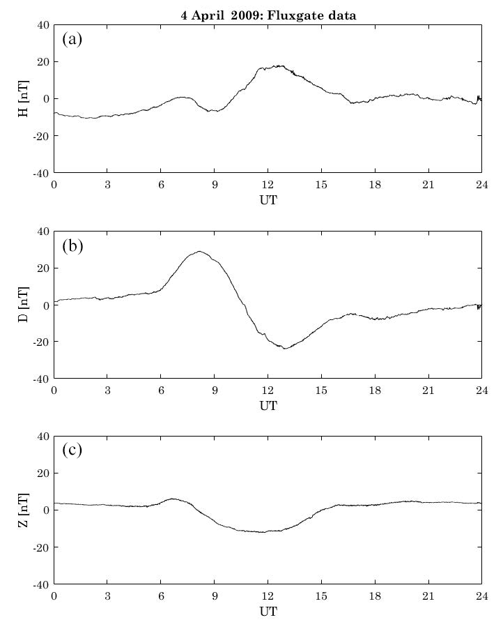
Figure 7 Geomagnetic field observations at L'Aquila ground station: (a) shows the H (north–south) component; (b) shows the D (east–west) component; (c) shows the Z (vertical) component. The observations show the typical Sq daily variations.

4 Discussion and conclusions

The correct identification of a background in the e.m. emission over seismic regions has a crucial role for the detection of possible signals related to earthquake or pre-earthquake activity. The algorithm presented here represents a new and very efficient technique to distinguish between instrumental, environmental, and external source signals from satellite observations. The efficiency of ALIF for both non-linear and non-stationary signal analysis, and peculiar frequency onset identification, has been proved in several works (i.e. Piersanti and Villante, 2016; Alberti et al., 2016, and references therein). In any event, its possible application to identify correctly the instrumental origin noise has never been presented before. Here, we showed that the coupling between ALIF and MSA represents a powerful tool to identify and remove noise from a signal. In fact, our method was able to determine all the noise frequencies declared in electric and magnetic field experiments of the DEMETER satellite (Lagoutte et al., 2005), such as 1 Hz in the E field (see Fig. 4). This signal is an effect of the instrumental disturbance, i.e. the sweeping voltage of the Langmuir probe (Lagoutte et al., 2005). Concerning the continuous 20 Hz signal detected in the magnetic field observations, we speculated that it can be attributed to one of the peaks of Shumann resonance in the ELF portion of the Earth's electromagnetic field spectrum generated and excited by lightning discharges in the cavity formed by the Earth's surface and the ionosphere (Barr et al., 2000, and references therein). In any event, Lagoutte et al. (2005) in their DEMETER satellite user guide manual certificated ∼20 Hz as a BANT (Boîtier Analogique et Numérique de Traitement) noise.

On the other hand, this paper presents a useful method for the correct selection of anomalous signals with respect to the evaluated background. The choice of using the ratio R_ϵ(ℓ) was to take into account possible anomalous energy enhancements as well as a new signal onset. In addition, the choice of a threshold equal to 3σ makes the anomaly selection as strong as possible and should exclude possible false positives. In any event, at this stage, a visual inspection of each anomalous signal detected is needed. Last but not least, an analysis of the geomagnetic index behaviour associated with a possible e.m. anomaly detected by our method is crucial. In fact, it is worth remarking that the external origin perturbations, in terms of solar activity, represent the principal disturbance of both the Earth's ionospheric electric and magnetospheric fields (Vellante et al., 2014; Piersanti et al., 2017a, and references therein).

In this context, the 333 Hz component, appearing when the DEMETER flew exactly over L'Aquila (Fig. 6), is not visible in the corresponding background (in terms of Kp and M indices – Fig. 4) and then may be an interesting anomaly. In fact, 4 April 2009 was characterized by very low geomagnetic activity, since the Sym-H index was between 8 and 10 nT, and the AE index was less than 95 nT. This confirms that 4 April 2009 was a solar quiet (Sq) day (Matsushida and Maeda, 1965; Chulliat et al., 2005). Sq is caused by the concurring contribution of a current system flowing in the so-called ionospheric dynamo region and of the induced telluric currents in the Earth's upper mantle. Briefly, their interaction gives rise to two pairs of vortices: two in the sunlit hemisphere and the other two in the dark one (Richmond et al., 1976; Shinbori et al., 2014). This is confirmed by the behaviour of the geomagnetic field observation at L'Aquila ground station (Fig. 7), which presents the typical Sq daily variation at middle/low latitude in April (De Michelis et al., 2010). In addition, the inspection of the solar wind conditions coupled with a map of auroral oval emission from the DMSP satellite taken at 20:34 UT (not shown) confirmed the absence of any disturbance of solar origin, such as substorm activity, that could affect the low–middle latitudes' magnetic and electric fields. Indeed, L'Aquila geomagnetic trace (Fig. 7) did not show any Pi2 wave activity for the entire day (Olson, 1999; Piersanti et al., 2017a). Moreover, no ELF perturbations are observed between 20:30 and 20:40 UT. As a consequence, we can reasonably assert that s^∗ cannot be related to any solar perturbation.

As a matter of fact, the relative Poynting vector S indicates a wave propagating from the ground to the ionosphere. The s^∗ peculiar polarization might be associated with a horizontal current system flowing at the ground, switched on by an anomalous ground impedance generated by the fault break. It is thought that the low-frequency components (ULF/ELF) of seismo-electromagnetic emission (SEME) waves generated by pre-seismic sources (such as local deformation of fields, rock dislocation and micro-fracturing, gas emission, fluid diffusion, charged particle generation and motion, electro-kinetic, piezo-magnetic and piezoelectric effects, and fair weather currents) are transmitted into the near-Earth space (Dobrovolsky, 1989; Teisseyre, 1997; Pulinets and Kirill, 2004; Sorokin, 2001). During their propagation through the solid crust, the SEME waves characterized by lower periods are attenuated. As a consequence, only low-frequency waves (in the ULF/ELF band) can go over the Earth's crust and propagate through the ionosphere–magnetosphere system with moderate attenuation (Bortnik and Bleier, 2004). Observations from the low-Earth orbit (LEO) satellite seem to confirm this scenario. In fact, pre-seismic variations of electric and magnetic fields and of ionospheric plasma temperature and density (Parrot, 1993; Chmyrev, 1997, Buzzi, 2007) have been observed from a few minutes to several hours (2–6 h) prior to earthquakes of moderate or strong magnitude (M>4.0). Unfortunately, no magnetotelluric measurements that could confirm or contradict our hypothesis were available for the event under investigation. In any event, it is interesting to emphasize that, repeating the same analysis for cells further north and south than the L'Aquila cell (not shown), no anomalous signal centred at 333 Hz was found. So, we are confident that what is seen on 4 April only occurred above L'Aquila and not elsewhere.

Interestingly, on 11 February 2009, a similar signal, characterized by lower (∼60 %) ϵ_rel and comparable polarization, was observed on both electric and magnetic field components. Despite the direction of S confirming that this signal also comes from the ground (${\mathit{\vartheta }}_{\mathrm{2}}=\mathrm{154.6}{}^{\circ }$ and ${\mathit{\phi }}_{\mathrm{2}}=\mathrm{6.4}{}^{\circ })$, nothing can be speculated as to its physical causes in this case. In fact, first of all, it is characterized by different solar activity conditions, with Sym-H between 40 and 50 nT, and AE between 150 and 200 nT. Last but not least, the satellite orbit was diurnal. Hence, to be consistent with our cell division method, 11 February 2009 cannot be compared to our quiet background or to the 4 April 2009 case event. In any event, its peculiar characteristics need to be investigated in a companion paper containing a statistical approach.

The analysis of the 4 April 2009 event showed that only through a multi-instrumental and multi-disciplinary approach can a reliable disentanglement of the earthquake effects from changes due to the physical processes that govern the ionosphere dynamic and natural EME be obtained.

This work could be considered as a suggested analysis approach for the forthcoming scientific phase of the first CSES mission (launched in February 2018, and still in the commissioning phase) aiming to reduce the lack of knowledge of lithosphere–ionosphere coupling. As soon as further applications, performed on different seismic events, reach the expected reliability, the proposed method could be used to compute the global background level (with 1 squared degree of resolution) for a direct real-time comparison of CSES in-flight data.