Latitude-dependent delay in the responses of the equatorial electrojet and S_q currents to X-class solar flares

We have analyzed low-latitude ionospheric current responses to two intense (X-class) solar flares that occurred on 13 May 2013 and 11 March 2015. Sudden intensifications, in response to solar flare radiation impulses, in the S_q and equatorial electrojet (EEJ) currents, as detected by magnetometers over equatorial and low-latitude sites in South America, are studied. In particular we show for the first time that a 5 to 8 min time delay is present in the peak effect in the EEJ, with respect that of S_q current outside the magnetic equator, in response to the flare radiation enhancement. The S_q current intensification peaks close to the flare X-ray peak, while the EEJ peak occurs 5 to 8 min later. We have used the Sheffield University Plasmasphere-Ionosphere Model at National Institute for Space Research (SUPIM-INPE) to simulate the E-region conductivity enhancement as caused by the flare enhanced solar extreme ultraviolet (EUV) and soft X-rays flux. We propose that the flare-induced enhancement in neutral wind occurring with a time delay (with respect to the flare radiation) could be responsible for a delayed zonal electric field disturbance driving the EEJ, in which the Cowling conductivity offers enhanced sensitivity to the driving zonal electric field.

Keywords. Ionosphere (equatorial ionosphere)

1 Introduction

During a solar flare event, a great enhancement in extreme ultraviolet (EUV) and X-ray radiation causes sudden and intense disturbances in the Earth's upper atmosphere. These disturbances are observed in the form of sudden increases in the ionospheric electron density in the D, E and F regions, reflecting in the ionospheric currents (Curto et al. 1994a, b, Xiong et al., 2011; Tsurutani et al., 2005; Manju et al., 2009; Nogueira et al., 2015; Abdu et al., 2017). The equatorial electrojet (EEJ) current system is also disturbed due to sudden increase in the solar ionizing radiation flux. Also, some studies have shown that in addition to large disturbances in the ionosphere, solar flares can also cause significant responses in the neutral density and temperature and dynamics of the thermosphere (e.g., Forbes et al., 2005; Sutton et al., 2006; Liu et al., 2007; Pawlowski and Ridley, 2008, 2009, 2011; Le et al., 2015).

The increase in the solar radiation during a solar flare events produces geomagnetic field disturbances, due to the sudden intensification in the global ionospheric current system caused by the flare-induced enhanced ionospheric conductivity (Rastogi et al., 1999; Moldavanov, 2002). The EEJ response under solar flare events has been extensively investigated and documented in the literature. Besides the sudden increase in the ionization density by the flare radiation, the EEJ enhancement is also shaped by the background electric field (Abdu et al., 2017; Zhang et al., 2017; Rastogi et al., 1999). In the present work, we analyze the responses of the ionospheric current system during two solar flare events that occurred near midday on 13 May 2013 and 11 March 2015; both events occur during geomagnetic quiet days. The solar flare of 13 May 2013 was classified as an X2.8 class event (the intensity peaking at 16:05 UT), and the solar flare of 11 March 2015 was classified as an X2.2 class event (the intensity peaking at 16:22 UT).

Table 1 Geographic and magnetic coordinate of the magnetometer stations.

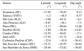
We have analyzed magnetometer data from Brazilian and Peruvian equatorial and low-latitude sites for an evaluation of the flare manifestations in S_q and EEJ currents. Table 1 shows a list of stations ordered by the dip angle, with their coordinates, from which magnetometer data are analyzed in this work. We have observed a delay from 5 to 8 min (2015 and 2013 events, respectively) in the occurrence of peak response in the strength of the magnetic effect of the EEJ current at the ground level (named EEJ ground strength for simplification) changes with respect to the peak response in the ground strength of the induced magnetic field due to the S_q current outside the magnetic equator (hereafter S_q ground manifestation for simplicity) modification which was nearly simultaneous with the peak in the flare X-ray flux. We seek an explanation for this delay by modeling the Cowling conductivity variations produced by the flare enhanced X-ray and EUV fluxes in the equatorial and low-latitude ionosphere close to midday. We used the Sheffield University Plasmasphere-Ionosphere Model at National Institute for Space Research (SUPIM-INPE; Bailey et al., 1978, 1993; Souza at al., 2013; Nogueira et al., 2013; Santos et al., 2016), which has been found to simulate realistically the equatorial–low-latitude ionosphere. The modeling results showed that the flare-induced temporal delays in the EEJ response (and in turn in its ground manifestation) cannot be attributed to a corresponding delay in the flare-induced enhanced Cowling conductivity development. We then examined if there is a difference in the integrated Cowling conductivity response to solar flare radiation at the two longitudes sectors where the data were analyzed. The possibility of any variation with height in the Cowling conductivity response were also examined since the EEJ and the S_q current flow at different altitudes. We present in Sect. 2 the methodology to obtain the variations in the horizontal component of the Earth's magnetic field (ΔH), representing the S_q and EEJ current systems, and the ionospheric simulation procedure using SUPIM-INPE. Section 3 deals with the results of analysis of the observational data and of SUPIM-INPE simulation runs and discussion of the results, and Sect. 4 presents the summary and conclusions.

2 Methodology

2.1 The ΔH variations representing the S_q and EEJ current strength

The geomagnetic field horizontal component (H) obtained from magnetometer data with 1 min resolution has been used. The H variations over the low-latitude stations, São Martinho da Serra, Cachoeira Paulista, São José dos Campos, Jataí, Cuiabá and Eusébio are used to examine the flare effect in the S_q variation. The H variations at the magnetic equatorial stations Tatuoca and Jicamarca are used to determine the flare time variations at the EEJ locations. The stations Piura, São Luís and Alta Floresta represent transition region between low latitudes and the dip equator. The H component variation due to ionospheric and magnetospheric currents was determined by subtracting the midnight values of the H component, considered as baseline values (due to the Earth's main field), from the H field at all local times (see Sect. 2 in Denardini et al., 2009, for detailed information). To determine the EEJ strength, which we have done for the Peruvian sector, the ΔH variation at an off-equator station, Piura (in this case), was subtracted from that over the dip equatorial station, Jicamarca.

2.2 Model simulations by SUPIM-INPE

We have modeled the field line-integrated Cowling conductivity using the SUPIM-INPE (Bailey and Sellek, 1990, 1997; Souza et al., 2000, 2013; Nogueira et al., 2013; Santos et al., 2016). The SUPIM-INPE solves the time-dependent equations of continuity, momentum and energy along magnetic field lines to obtain the electron and ion densities of the low-latitude ionosphere. The calculations use terms of ion production, ion loss due to chemical reactions, thermal conduction, photoelectron and frictional heating and local heating/cooling mechanisms. The transport effects include the ambipolar and thermal diffusion, ion–ion, ion–neutral and electron–neutral collisions, thermospheric neutral winds (Hedin et al., 1996) and vertical plasma drift (Scherliess and Fejer, 1999).

The SUPIM-INPE calculates the electron and ion densities using the ion production rate due to the solar X-rays and EUV radiation, with 1 min time resolution that permits the representation of the rapid variation in the solar radiation flux under the flare conditions. The ionizing radiation fluxes input to the model are those of the solar EUV at 43 wavelength bands (from 0.5 to 105.00 nm) from the Flare Irradiance Spectral Model (FISM; Chamberlin et al., 2007, 2008). The NRLMSISE-00 neutral atmospheric model (Picone et al., 2002) is used as input in SUPIM-INPE. We have used a version of the SUPIM-INPE for which the lowest altitude limit of calculation was extended to 90 km from its original limit of 120 km. This model is designated as SUPIM -INPE.

The electron/ion densities resulting from the model were used to calculate the magnetic field line-integrated Pedersen and Hall conductivities based on the formulation by Haerendel and Eccles (1992). The local Pedersen and Hall conductivities, σ_P and σ_H, are given by

$$\begin{array}{ll}{\displaystyle }& {\displaystyle }{\mathit{\sigma }}_{\mathrm{P}}={\displaystyle \frac{e{n}_{\mathrm{e}}}{B}}\left({\mathit{\mu }}_{\mathrm{Pi}}-{\mathit{\mu }}_{\mathrm{Pe}}\right),\\ {\displaystyle }& {\displaystyle }{\mathit{\sigma }}_{\mathrm{H}}={\displaystyle \frac{e{n}_{\mathrm{e}}}{B}}\left({\mathit{\mu }}_{\mathrm{Hi}}-{\mathit{\mu }}_{\mathrm{He}}\right),\end{array}$$

where μ_Pe,i and μ_He,i, are the Pedersen and Hall mobilities, respectively, of the electrons (sub-index “e”) and ions (sub-index “i”), e is the basic charge, n_e is the electron density and B is the geomagnetic field. The Pedersen and Hall mobilities are defined as

$$\begin{array}{ll}{\displaystyle }& {\displaystyle }{\mathit{\mu }}_{\mathrm{Pi},\mathrm{e}}={\displaystyle \frac{k_{\mathrm{i},\mathrm{e}}}{\mathrm{1}+k_{\mathrm{i},\mathrm{e}}^{\mathrm{2}}}},\\ {\displaystyle }& {\displaystyle }{\mathit{\mu }}_{\mathrm{Hi},\mathrm{e}}={\displaystyle \frac{k_{\mathrm{i},\mathrm{e}}^{\mathrm{2}}}{\mathrm{1}+k_{\mathrm{i},\mathrm{e}}^{\mathrm{2}}}},\end{array}$$

where k_i,e is the ratio between gyrofrequency to the collision frequency given by

$$k_{\mathrm{i},\mathrm{e}}={\displaystyle \frac{{\mathrm{\Omega }}_{\mathrm{i},\mathrm{e}}}{{\mathit{\nu }}_{\mathrm{in},\mathrm{en}}}}.$$

In order to simulate a realistic representation of the conductivities, we have added the electron–neutral collision contribution to the conductivity formulation in the SUPIM-INPE. The collision frequency equations of ion–neutral and electron–neutral were obtained from Kelley (2008).

Finally, the field line-integrated conductivities were obtained as

$${\mathrm{\Sigma }}_{\mathrm{H},\mathrm{P}}=\mathrm{2}{R}_{\mathrm{E}}L\underset{\mathrm{0}}{\overset{{\mathit{\zeta }}_{\mathrm{m}}}{\int }}{\mathit{\sigma }}_{\mathrm{H},\mathrm{P}}{\left(\mathrm{1}+\mathrm{3}\mathit{\zeta }\right)}^{\mathrm{1}/\mathrm{2}}\mathrm{d}\mathit{\zeta }.$$

The Cowling conductivity ∑_C is calculated using the expression

$${\mathrm{\Sigma }}_{\mathrm{C}}={\mathrm{\Sigma }}_{\mathrm{P}}\left[\mathrm{1}+{\left({\displaystyle \frac{{\mathrm{\Sigma }}_{\mathrm{H}}}{{\mathrm{\Sigma }}_{\mathrm{P}}}}\right)}^{\mathrm{2}}\right],$$

where ζ=sin λ (λ is the dip latitude). The integration limits starts from 0 at the equator.

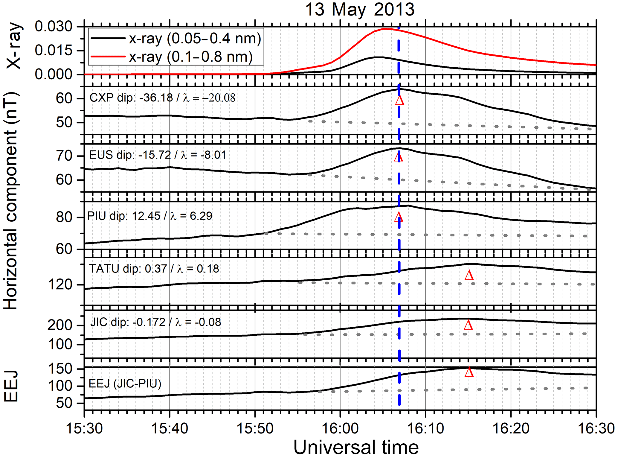
Figure 1 Flux variations in two X-ray bands (0.05–0.4 and 0.1–0.8 nm) and S_q and EEJ currents response to X-class flare event of 13 May 2013 (top panel) and the corresponding variations in the S_q current and in the EEJ plotted as the H variations over low-latitude and dip equatorial stations in Peru and Brazil.

3 Results

3.1 Observational data

Figure 1 shows, in the top panel, the X-ray flux variation as recorded by the Geostationary Operational Environmental Satellite (GOES 15), from 15:30 UT up to 16:30 UT, on 13 May 2013 (a geomagnetic quiet day, daily ∑Kp = 8), in which the flare time flux enhancement (during this X2.8 class event) may be noted. Simultaneous variations in the horizontal components of the Earth's magnetic field as measured by a number of magnetometers in South America are shown in the following successive panels. We note the solar flare X-ray flux peaking at 16:05 UT, when it happened to be just past midday over Brazil, and before midday over Peru (local standard time in Brazil is UT−3, and in Peru UT−5). The H variations during daytime are shown for Cachoeira Paulista (CXP), Eusébio (EUS), Piura (PIU), Tatuoca (TATU) and Jicamarca (JIC), as well as the EEJ strength over Jicamarca represented by the difference in the horizontal component between Jicamarca and Piura. The dip lat and magnetic inclination angle for the respective stations are shown in each panel (See also, Table 1).

Figure 2 Plots similar to those of Fig. 1, but for the X-class flare of 11 March 2015.

In response to flare enhancement in the X-ray flux, the H component shows a strong and rapid increase at all the stations. This sudden intensification in the H component is a signature of the response of the global ionospheric S_q and the EEJ current systems to the sudden conductivity enhancement, caused by the flare X-ray ionization (Richmond and Venkateswaran, 1971; Rastogi et al., 1999). The red arrows mark the time of the peaks in H intensification at each of the stations. The peaks in the H intensification at CXP, EUS and PIU can be seen to be occurring almost simultaneously (within about 2 min) with the peak in the X-ray intensity. However, the corresponding H intensification over TATU and JIC that are dip equatorial stations peaked 8 min after at CXP, EUS and PIU (or ∼ 10 min after the peak in X-rays). Correspondingly, the EEJ over Jicamarca plotted in the bottom panel also showed a delay of 8 min (or 10 min after peak in X-rays). With respect to the peak in the S_q response, the delay in the EEJ peak may be noted as being 8 min, which is a significant time delay.

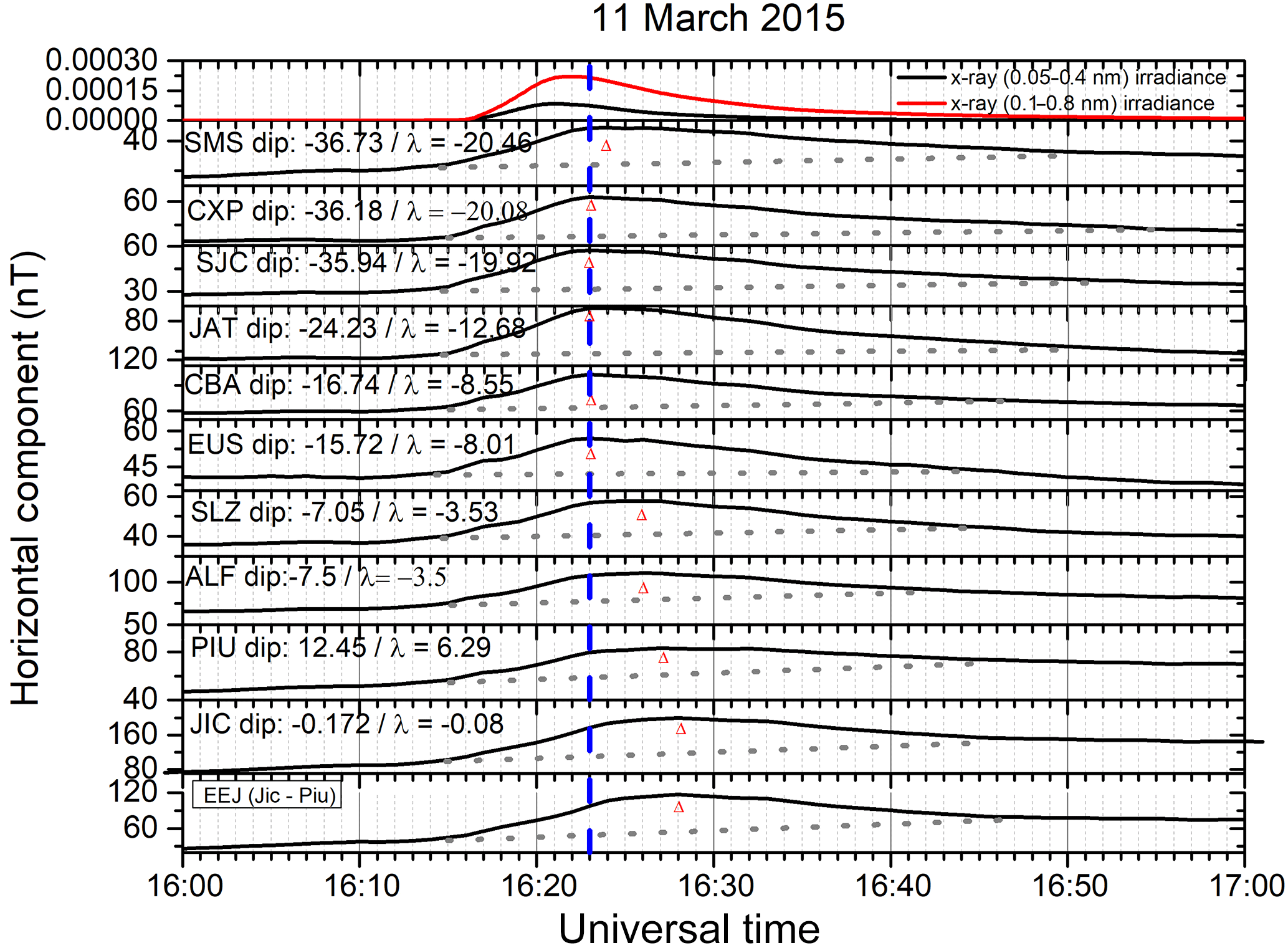
Figure 2 is similar to Fig. 1, but corresponds to the solar flare event of 11 March 2015 (a geomagnetic quiet day, daily ∑Kp = 16). The H component variations for this event are presented in this figure for SMS, CXP, SJC, JAT, CBA, EUS, SLZ, ALF, PIU and JIC, as well as the EEJ strength over Jicamarca. There were no data for Tatuoca (dip equator) for this event. This figure also clearly shows the geomagnetic signatures of the global ionospheric S_q current system intensification as well as the EEJ intensification, due to an X-class flare. In this case, as was noted in Fig. 1, we can see that the S_q current intensification peaked near the X-ray peak (with a delay of around 2 min) at SMS, CXP, SJC, JAT, and EUS. However, starting at SLZ and ALF, which are closer to the dip equator the delay appears to increase, and at Jicamarca, a dip equatorial station, we note a delay of 5 min in the EEJ peak with respect to the peak in S_q. Thus the results in Figs. 1 and 2 demonstrate that the response to solar flare enhanced radiation is somewhat slower in the EEJ current than it is in the S_q current system. This is manifested in the form of a delay in the EEJ response peak with respect to the flare intensity peak, which is larger than the corresponding delay observed in the S_q response peak with respect to the solar flare intensity peak.

Table 2 Summary of the magnetic signatures during the solar flare.

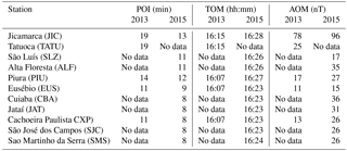
In Figs. 1 and 2 we have drawn, shown in the gray dashed line, the quiet time profile of the H component for each station in order to define the period of increase (POI), time of maximum (TOM) and amplitude of the maximum (AOM). The observations are summarized in Table 2.

From Table 2 we can observe that period of increase is sorted by dip angle, showing that the peak increase of the H component occurs later at dip equator stations in comparison with no equatorial stations, which is in agreement with the time of maximum. We also can observe that the time of maximum occurs at 16:15 and 16:28 at dip equatorial stations during the solar flares of 2013 and 2015, occurring with 8 and 5 min delays to the non-equatorial stations, respectively. It is also interesting to observe that the amplitude of maximum is larger at the magnetic equator; however it is not sorted by dip angle.

Nogueira et al. (2015) had observed such delay, but no detailed analysis or interpretation was attempted. In an attempt to obtain a better clue on the nature of the delay and to seek an understanding of its possible cause, in the present work, we have carried out detailed modeling with sufficient temporal and spatial resolutions of the E-layer conductivities during the course of the flare.

3.2 Modeling results by SUPIM-INPE

The field line-integrated conductivities, ∑_P and ∑_H, and hence the Cowling conductivity were calculated using the results obtained from the SUPIM-INPE simulation of the low-latitude ionosphere at 1 min and 2.5 km resolutions. Figure 3 shows the results of two theoretical experiments for the integrated Cowling conductivity on 13 May 2013 over 45^∘ W. The bottom left panel shows the integrated Cowling conductivity modeled considering constant background X-ray and EUV fluxes (no flare condition) shown in the top left panel of Fig. 3, for three wavelengths. The right bottom panel shows the integrated Cowling conductivity as calculated using the flare enhanced X-ray and EUV (in the wavelength band 0.5–105.00 nm) flux variations shown in the top right panel. The Flare Irradiance Spectral Model (FISM) was used in the simulation at 1 min time cadence to achieve sufficient resolution during the solar flare event.

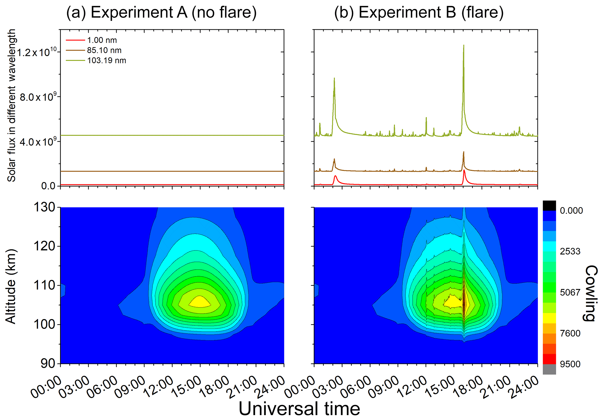
Figure 3 The magnetic field line-integrated Cowling conductivity modeled using the SUPIM-INPE for (a) non-flare conditions and (b) by including the flare radiation for the X-class flare of 13 May 2013. The SUPIM-INPE simulation was done for equatorial ionosphere at 45^∘ W.

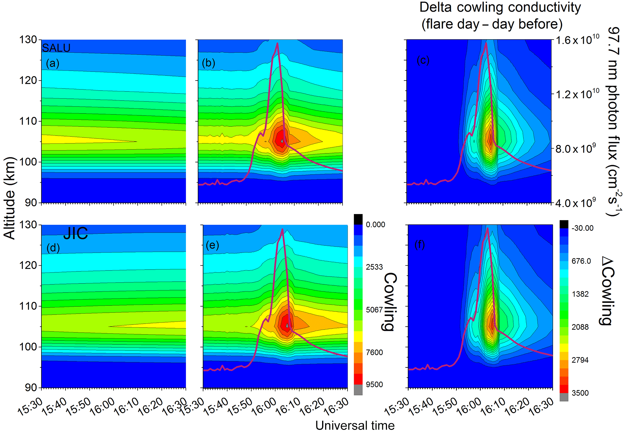
Figure 4 Field line-integrated Cowling conductivity variations over longitudes of São Luís and Jicamarca plotted during the time span (15:30–16:30 UT) covering the X-class flare of 13 May 2013. The left panels show the ∑_C variations without flare radiation, the middle panels show the variations when flare radiation is included, and right panels show the difference between the left and middle panels, that is, the extra effect produced by the flare radiation. The flare X-ray flux variation is also plotted (red curve) in the middle and right panels. W.

The model results in Fig. 3 shows the field line-integrated Cowling conductivity variation for the duration of entire day plotted as a function of the apex height over the dip equator. We note very low conductivity during the night as to be expected. A rapid rise in the conductivity marks the sunrise, which is followed by the daytime increase in its values that peak at midday (UT−3). In its height variation the ∑_C peaks in the region of 105–107 km, which is in accordance with results from many observational and theoretical studies (Richmond, 1973; Haerendel and Eccles, 1992; Kelley et al., 2012). In the right panels, where the time variation of the solar flux is considered, we can clearly note the sensibility of the integrated Cowling conductivity to small changes in the EUV flux variation. The feature to be noted foremost is the large and sudden increase in the conductivity at about 16:05 UT associated with the X-class solar flare.

Figure 4 shows the ∑_C variations as a function of apex heights from 90 to 130 km (similar to Fig. 3) but on an expanded timescale (from 15:30–16:30 UT) surrounding the X-class flare, for São Luís and Jicamarca. Figure 4a and d show conductivity variations for the non-flare condition while the panels (b) and (e) show such variations when flare radiation is included. The difference between flare condition and non-flare conditions are shown in panels (c) and (f) for 45^∘ W of São Luís and for 75^∘ W of Jicamarca, respectively. The quiet time peak in ∑_C occurs around 105–107 km. It may be noted that during the calculation window (15:30–16:30 UT shown here), under non-flare conditions, the ∑_C peak value decreases with time over SLZ, whereas it increase with time over Jicamarca, a contrasting feature caused by the 30^∘ difference in longitude between the two locations, with the LT at SLZ ahead of JIC by 2 h.

In Fig. 4b and e, we note, coincident with the rapid increase in the solar flare radiation, a sudden enhancement on the integrated conductivity at both stations, peaking at 16:05 UT and 105 km height. The peak in ∑_C follows closely (within about 2 min) the peak in the X-ray flux. The rate of increase and decrease in ∑_C follows closely that of the flare X-ray flux variation, both during the growth and decay phases of the event. Further, one can note a slower decay rate of ∑_C (after the X-ray peak flux) over Jicamarca as compared to that over São Luís (perceivable in the orange contour at about 105 km extending up to 16:30 at Jicamarca but less so at São Luís), which is due to the 2 h local time difference between the two locations, mentioned above. However when the difference between the flare day and non-flare day contours is taken, we note in Fig. 4c and f that no difference in ΔΣ_C variation is present between the two locations (separated in longitude). This results shows that the apparently slower decay rate of ∑_C at Jicamarca was due to the pre-noon hour of flare occurrence there when the background conductivity increases with LT, in contrast to the post-noon hour at São Luís when the LT-dependent decrease in background conductivity contributes to a faster decay rate. It may be noted further (in Fig. 4c and f) that the decay in the conductivity after attaining its peaks appears to follow the decay rate of the X-ray flux after its peak intensity. However, the value of ∑_C corresponding to a specific value of the X-ray flux is larger during the decay phase (after the X-ray peak) than during the growth phase (before the X-ray peak). Thus the flare effect on the integrated conductivity appears to be longer lasting than the flare radiation, which is in agreement with previous results based on electron density measurements (see, for example, Liu et al., 2007). Since the EEJ intensity is directly related to the value of the ∑_C, these results do not directly explain the additional delay in the EEJ peak with respect to the peak in S_q current, or with respect to the flare radiation, observed in Figs. 1 and 2, because no corresponding delay in ∑_C is found in the model results.

Figure 5 Altitudinal variation of the solar flare effect on the current density.

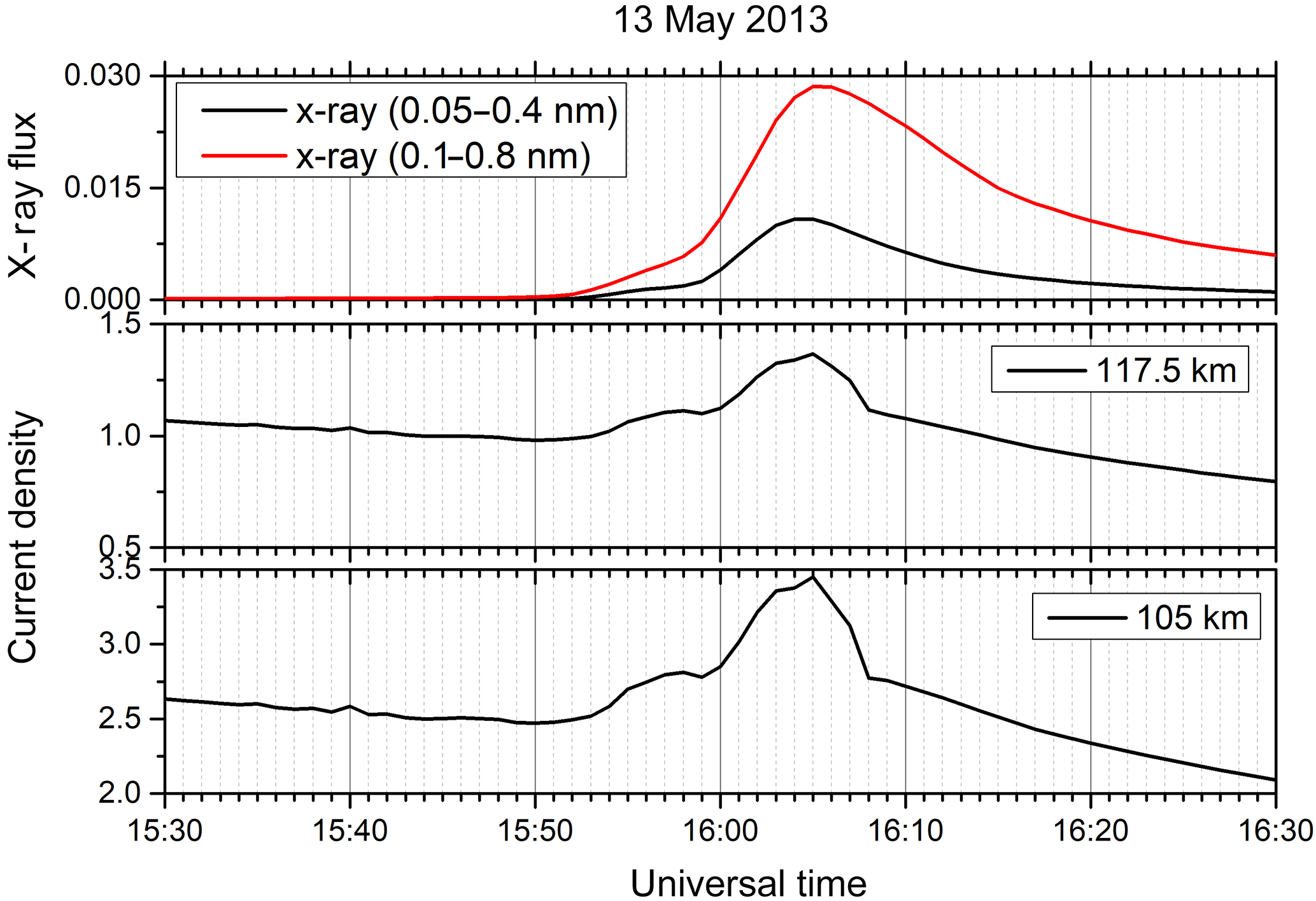
In order to better relate the results of the model with the magnetometer data, Fig. 5 shows the altitudinal variation of the current density, $J_{\mathit{\varnothing }}=E_{\mathit{\varnothing }}{\sum }_{\mathrm{C}}$. By using SUPIM-INPE we have calculated the integrated Cowling conductivity and by using the Fejer et al. (2008) empirical model we have obtained the zonal electric field, by considering that a vertical drift velocity of about 40 m s⁻¹ corresponds to an east–west electric field of 1 mV m⁻¹ (Fejer et al., 1979). Figure 5 shows the possible existence of altitudinal variation in the response time of the current density that could help to explain a corresponding height-dependent delay at the EEJ peak height occurring at 105 km with respect to the S_q currents outside the EEJ occurring at about 117.5 km. The results of these calculations are plotted in Fig. 5 at 1 min resolution from 15:30 to 16:30 UT, in which in the top panel the X-ray variation is shown, followed by J_∅ variations at 105 km and 117.5 km heights, respectively. It may be noted in the figure that the peak current density values occur at the same time at all the heights, and therefore the observed time delay in the EEJ peak cannot be explained in this way either. By assuming that ∑_C is calculated by using the solar radiation time variation associated to the solar flare, but with no corresponding variation found on the electric field model of Fejer et al. (2008), in the following section we investigate a possible dependence of the zonal electric field disturbance as responsible for the observed time delay in the EEJ peak.

4 Discussion and conclusions

The absorption of the flare enhanced radiation in X-rays and UV/EUV bands in the atmosphere results in complex processes that modify the ionosphere as well as the background neutral atmosphere. The direct effect through photo ionization that causes prompt enhancement in density is responsible for conductivity variations that should produce also prompt responses in the S_q and EEJ currents. However, as discussed above, we observe a delay in the response of the EEJ to the flare radiation enhancement, the delay being significantly larger, by ∼ 5–8 min, than that seen in the response of the S_q current to the flare radiation. We are unsure regarding the mechanism which explains the observed delay. However, in search of a plausible explanation we will examine some aspects of the background thermospheric response to the flare radiation. Photoelectron ionization, dissociation and excitation of the neutral atmosphere/thermosphere are responsible for heating and therefore for the density enhancements that take place at a slower rate than the initial photo ionization rate. The flare-induced thermospheric density response during the severe storms of October–November 2003 has been studied using CHAMP satellite observations at 400 km by Sutton et al. (2006) and Liu et al. (2007) and using Global Ionosphere-Thermosphere Model (GITM) by Pawlowski and Ridely (2008).

Enhancements of the thermosphere neutral density of up to 50 % that can occur with a time delay of 1–2 h have been verified in those studies. In particular, the model study by Pawlowski and Ridely (2008) has shown flare-induced density and temperature enhancements, with the effect decreasing from the 400 km (CHAMP satellite height) down to 110 km. It is not clear if these effects could drive winds in the lower thermosphere (in the height region of the S_q current and EEJ) to the extent necessary to modify the dynamo electric field. If modification of the E-region dynamo electric field (by such a hypothetical wind) is possible, then it should occur with a time delay that also produces a delay in the EEJ response with respect to the flare radiation enhancement, as explained below.

The zonal current density in the electrojet can be represented as

$$J_{\mathit{\varnothing }}=E_{\mathit{\varnothing }}{\sum }_{\mathrm{C}}.$$

E_∅ is the zonal electric field arising from E-layer dynamo; ∑_C is the field line-integrated Cowling conductivity as defined in Sect. 2. The calculation of the integrated conductivities using the low-latitude ionosphere simulated by the SUPIM-INPE shows that at the center of EEJ, in the height region of 105–107 km, the peak value of ∑_C is a factor of approximately 400 higher than that of ∑_P. This would imply that for a given value of E_∅ the response to solar flare-induced ionization enhancement is at least 400 times more sensitive at the center of the EEJ (due to ∑_C enhancement) than it is in S_q current (which is limited only to ∑_P enhancement). The impulsive increase of solar flare radiation could cause an increase in neutral density and temperature, as mentioned before, at E-layer heights (even though it may be of a small degree) that could modify the wind, thereby causing disturbances in the zonal electric field (E_∅). Such disturbance in E_∅ should occur at a rate somewhat slower than that of the flare enhancement in the conductivity. Because of the enhanced Cowling conductivity (∑_C) of the EEJ, the response to a slower change in the E_∅ could be more readily perceivable (recognizable) in the EEJ than possible in the S_q current. In this way the delayed peak in the EEJ, as compared to that in the S_q or the flare radiation, observed in the data can be tentatively explained. Our conclusion is supported by Zhang et a. (2017), who verified that the dayside upward vertical drifts have significant decreases during seven solar flares events, showing that the solar flares induce a westward disturbance in the electric field.

Thus, we propose that the sluggishness in the response of the neutral density and wind to the absorption of flare radiation could be responsible for the delay of a few to 8 min, in the background EEJ zonal electric field as observed by magnetometers.