the Creative Commons Attribution 4.0 License.
the Creative Commons Attribution 4.0 License.
 | 25 Jan 2018
Modelling the main ionospheric trough using the Electron Density Assimilative Model (EDAM) with assimilated GPS TEC
James A. D. Parker
S. Eleri Pryse
Natasha Jackson-Booth
Rachel A. Buckland
The main ionospheric trough is a large-scale spatial depletion in the electron density distribution at the interface between the high- and mid-latitude ionosphere. In western Europe it appears in early evening, progresses equatorward during the night, and retreats rapidly poleward at dawn. It exhibits substantial day-to-day variability and under conditions of increased geomagnetic activity it moves progressively to lower latitudes. Steep gradients on the trough-walls on either side of the trough minimum, and their variability, can cause problems for radio applications. Numerous studies have sought to characterize and quantify the trough behaviour.
The Electron Density Assimilative Model (EDAM) models the ionosphere on a global scale. It assimilates observations into a background ionosphere, the International Reference Ionosphere 2007 (IRI2007), to provide a full 3-D representation of the ionospheric plasma distribution at specified times and days. This current investigation studied the capability of EDAM to model the ionosphere in the region of the main trough. Total electron content (TEC) measurements from 46 GPS stations in western Europe from September to December 2002 were assimilated into EDAM to provide a model of the ionosphere in the trough region. Vertical electron content profiles through the model revealed the trough and the detail of its structure. Statistical results are presented of the latitude of the trough minimum, TEC at the minimum and of other defined parameters that characterize the trough structure. The results are compared with previous observations made with the Navy Ionospheric Monitoring System (NIMS), and reveal the potential of EDAM to model the large-scale structure of the ionosphere.
Keywords. Ionosphere (midlatitude ionosphere; modelling and forecasting) – radio science (ionospheric physics)
- Article
(4760 KB) - Full-text XML
- BibTeX
- EndNote


The main ionospheric trough is a prominent and persistent depletion in the terrestrial ionized atmosphere, residing essentially between the dynamic high-latitude ionosphere on its poleward side and the more benign mid-latitude region on its equatorward side. The feature, which is also referred to as the mid-latitude trough, has been studied extensively over several decades with Muldrew (1965) being the first using topside sounder data. Reviews of early studies were conducted by Moffett and Quegan (1983) and Rodger et al. (1992). The lower trough densities are normally bounded by a steep ionization density gradient on the poleward wall and a prominent but shallower gradient on the equatorward side. The characteristics are elongated in longitude. When observed in Europe, as for example by Krankowski et al. (2009), the feature normally first occurs in late afternoon at latitudes poleward of 60∘ latitude. It then moves progressively equatorward through the night reaching its most equatorward latitude in pre-dawn hours. With the increasing sunlight at dawn, ionization production results in increased densities in the trough and the apparent rapid retreat of the feature to higher latitudes with the trough minimum being typically at 65∘ corrected geomagnetic latitude at 08:00 LT in the results of Krankowski et al. (2009). A large-scale trough also features in the post-noon high-latitude dayside ionosphere (Kersley et al., 1997). It also comprises a band of lower densities confined in latitude but extended in longitude. This trough has not been studied so widely as the nightside main trough at mid-latitudes, but it has been suggested that it is an extension of the mid-latitude night-time trough back to earlier local times and higher latitudes (Pryse et al., 2005; Moffett and Quegan, 1983). Interest in the trough occurs in applications of ionospheric radio propagation, largely driven by the influence of the feature on the propagation of high-frequency radio signals as shown along the oblique subauroral paths considered by Andreev et al. (2006).
Studies of the trough have spanned several decades. Early work used topside electron density profiles from Alouette 1 ionograms to identify the trough and its dependency on geomagnetic activity (Rycroft and Burnell, 1970). Bates et al. (1973) focussed on the poleward edge of the trough under quiet geomagnetic activity, where the maximum electron density at the trough wall in the F region was some 1∘ latitude equatorward of the visible aurora. In later years, the dependencies of the trough on other parameters have been investigated, for example on season and solar activity (Ishida et al., 2014), geomagnetic conditions (Werner and Prölss, 1997) and longitude (He et al., 2011; Whalen, 1989). Many studies have aimed to characterize trough production and properties. For example, Spiro et al. (1978) related the subauroral trough to ionospheric decay in the region of slow plasma drift in the night-time sector. Zou et al. (2011) used Global Positioning System (GPS) vertical total electron content (VTEC) to investigate the dynamics of the trough under magnetic substorm activity and found that the poleward wall of the trough moved rapidly equatorward at the substorm onset because of increased particle precipitation, causing the trough to become narrower or even disappear. Yizengaw and Moldwin (2005) used global ionospheric maps of TEC obtained from measurements by a network of GPS receivers and extreme ultraviolet images of the Imager for Magnetopause-to-Aurora Global Exploration (IMAGE) Earth satellite to show agreement between the global positions of the mid-latitude trough and the plasmapause, implying that both features were on the same field lines. Electron density measurements by the Dynamics Explorer 2 (DE 2) satellite, at altitudes between 300 and 1000 km, were used by Werner and Prölss (1997) to develop two empirical models for the trough minimum invariant latitude as a function of magnetic local time (MLT), for the mid- and the high-latitude troughs. Feichter and Leitinger (2002) used the same DE 2 data set to model other properties of the trough including parameters of trough depth, width and steepness of trough walls. For this they also used the COSTprof electron density model (Hochegger et al., 2000) to map the densities measured at the DE 2 altitudes to values at the peak of the F region, owing to the eccentric orbit of the satellite covering a range of heights.
The main ionization trough has been studied using many different observing techniques. Methods of observation include the following: ionospheric sounders such as the networks considered by Whalen (1987, 1989); incoherent scatter radar, which can reveal the latitudinal structure of the trough and associated ionization temperature characteristics (Voiculescu et al., 2010); satellite TEC observations, for example by the Navy Ionospheric Monitoring System, NIMS (Kersley et al., 2004); and ionospheric tomography reconstruction using NIMS TEC observations (Pryse et al., 1993). In more recent years TEC measurements using GPS radio transmissions have been used to observe and study the trough, for example Krankowski et al. (2009) who used GPS observations from a network of receiving stations in Europe. Each of the observing techniques has its strengths and limitations. Incoherent scatter radars provide information on the electron density structure, electron and ion temperatures, and ion drift velocity. Observables by multiple radars can be combined for enhanced investigations of the trough structure and its evolution with time. For example, Hedin et al. (2000) used observations by the EISCAT Svalbard radar and the ultra-high frequency (UHF) and very-high frequency (VHF) mainland EISCAT radars in northern Scandinavia in a comparison with models of the trough minimum. The drawback of such incoherent scatter radar systems is that they are expensive and are located at specific locations with limits to the observing geometry. Radio tomography has also been used to image the latitudinal structure of the trough. The method in this case suffers from limited ray-path geometry set by the configuration of the satellites and receivers (Yeh and Raymund, 1991) and requires a priori information to support the reconstruction process (Raymund et al., 1993). In another inversion application Mitchell and Spencer (2003) presented an algorithm using GPS observations that yielded the time-evolving, three-dimensional ionospheric electron concentration. Their Multi-Instrument Data Analysis System (MIDAS) has proven successful for ionospheric imaging; however, there are still limitations, with some topside features being masked when influenced by lower ionosphere dynamics (Jayawardena et al., 2016).
Of particular interest to this current study is the measurement of TEC by GPS satellites using differential carrier phase (Horvath and Crozier, 2007). GPS propagation has been used increasingly for ionospheric observation. The satellites orbit at altitudes of approximately 20 200 km and inclinations of about 55∘ (Hoffmann-Wellenhoff et al., 2000). These transmit two phase-coherent signals at frequencies of 1575.42 MHz (L1 signal) and 1227.6 MHz (L2 signal). A radio receiver on the ground has up to 10 satellites in its field-of-view at any one time and can be used to measure the TEC along the satellite-to-receiver paths. The system was used in the statistical study of Yang et al. (2015) to investigate the trough dependency on season, geomagnetic activity and solar conditions. Consideration was given to the position of the trough minimum, the trough depth and width.
The investigation presented in this current paper is the first study to model and analyse the trough by assimilating GPS differential phase data into the Electron Density Assimilative Model (EDAM). EDAM (Angling and Cannon, 2004; Angling and Khattatov, 2006) is an operational system developed by QinetiQ for real-time monitoring of the ionosphere. EDAM is currently the only validated UK model that offers global electron density grids. The modelled trough is described in terms of a few identified parameters including the trough minimum and set points on the trough walls. Statistical analysis of these parameters, in turn, allowed the evaluation of EDAM to operate in the vicinity of deep ionospheric depletions with sharp latitudinal gradients on the trough walls.
The trough parameters modelled by EDAM are compared with observations of the earlier study (Pryse et al., 2006), which used multi-station measurements of the phase-coherent radio signals from the satellites of NIMS. In this earlier study TEC observations at three ground receivers in the UK, aligned in longitude but separated in latitude, were used to image the trough by tomographic reconstruction. The data used were recorded over a time period from September 2002 to August 2003. The current EDAM study aims at providing a fair comparison with the previous study, with sufficient data points to allow for the evaluation of the ability of EDAM to image steep ionospheric gradients. The study is not intended to provide a full statistical analysis of the seasonal dependency of the trough nor of the dependency of the trough on solar cycle activity. The data for the current study were taken from broadly the same period as the earlier study, thus keeping similar conditions of solar activity (10.7 cm solar flux). The earlier study had considered only cases where the trough was prominent. Relatively few troughs had been identified in the summer and therefore no seasonal variations in trough behaviour could be established. To keep similarity to the earlier study, summertime troughs were also not considered in the current study. The troughs were therefore confined to the equinox and winter period, and avoided the times of high solar illumination angles. It was deemed that the data set covering the autumn equinox period to winter (September to December 2002, inclusive) contained sufficient cases for a fair comparison. The period provided approximately 1950 latitudinal profiles of the trough, which was significantly larger than the 618 troughs of the earlier NIMS study. The period also provided data that were representative of the general behaviour of the prominent troughs of the earlier paper, with the four months including autumn, a season where the trough is prominent (Lee et al., 2011). The use of the four months as giving a fair representation of the prominent trough is reinforced in Fig. 6 of Le et al. (2017), where the data at 04:00 MLT for months 9 to 12 are representative of the prominent trough, in particular under low Kp. TEC characteristics of the summertime trough modelled by EDAM in June 2002 are presented in Sect. 5, which are different to those considered in the main study.
EDAM is an ionospheric model that assimilates data sources into a background model, currently provided by the International Reference Ionosphere 2007 (IRI2007; Bilitza et al., 2006). EDAM is capable of using any version of IRI as the background model, but IRI2007 is used in this study as it is the only version of IRI to have been validated with EDAM. The model assimilates ionospheric observations to generate global (or regional) 3-D representations of ionospheric electron density. An assimilation time step of 15 min has been used and the electron density differences between the voxels of the analysis and the background model are propagated from one time step to the next by assuming persistence combined with an exponential decay. The assimilated data sources used in the current study were GPS TEC measurements along satellite-to-ground paths. Previous studies (e.g. Angling and Jackson-Booth, 2011; Feltens et al., 2011) have shown that EDAM can accurately represent the ionosphere using GNSS data.
The EDAM assimilation process applies a weighted, damped least mean squares estimation between the background ionosphere and the observations, with the background being modified by the observations. The background grid provided by IRI2007 is modified progressively by each step of the assimilation process so that the model becomes increasingly aligned with the current observations. As each step of the process corresponds to a time interval of 15 min, observations during the 15 min are used in the assimilation step. There is also provision in the EDAM process to gradually return the modelled electron density to the IRI2007 electron density values for the time of interest, of relevance when there are no observations to update the grid values.
Each step in the EDAM assimilation process may be represented by Eq. (1).
where xa is the matrix of the electron density in the grid after an assimilation step, xb is the electron density of the current background model, y is the TEC observation matrix and H(xb) is the matrix of the TEC calculated through the current background model along the same path as the observations. K is a weighting matrix that controls the balance between the influence of the observations and the damping process, which applies an exponential decay to gradually revert the electron densities to IRI2007 values. The time constant for the decay of 4 hours is hard-coded into the model; so if the assimilated data are interrupted for this length of time, the model will revert to the IRI2007 model at the time of interest. However, this decay time was immaterial in this current study, with the decay being irrelevant as data were assimilated throughout the study period. The output electron density was restricted to the European region of interest, 45.0 to 70.0∘ N latitude and −20.0 to 40.0∘ E longitude.
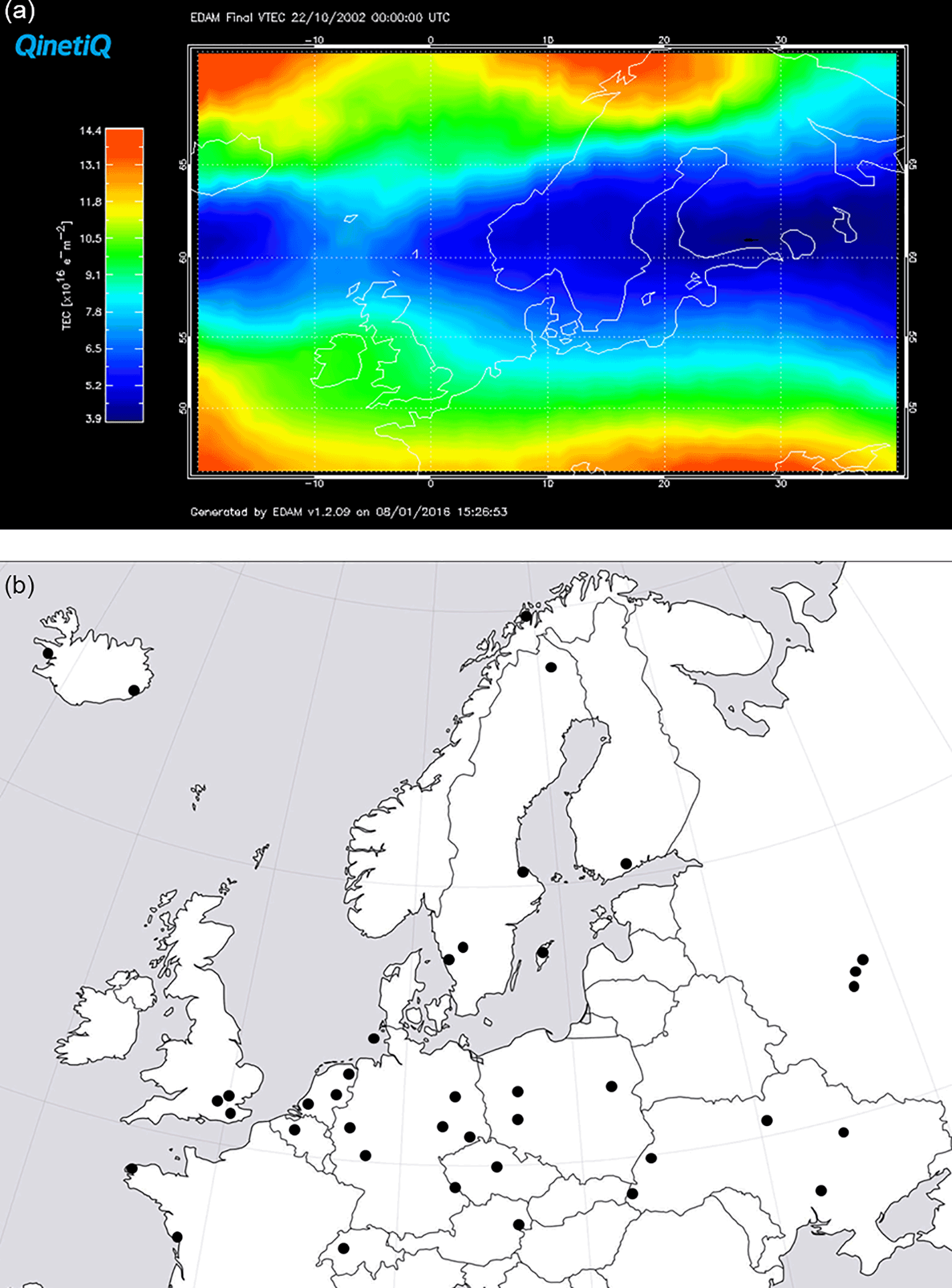
Figure 1(a) Vertical TEC through the EDAM grid at 00:00 UT on 22 October 2002. The spatial coverage of the figure extends from −20.0 to 40.0∘ E and from 45.0 to 70.0∘ N. The trough extends across the field-of-view with its minimum TEC of approximately 4.0 TECU near 60.0∘ N. (b) A map showing the locations of the receivers used in the assimilation.
The voxels of the model grid are each of dimensions 4∘ latitude by 4∘ longitude, but through interpolation electron density values can be obtained at a higher resolution with the values obtained in the current study being at 1∘ intervals of latitude and longitude in geographic co-ordinates. The vertical dimension of the voxels is 10 km. For the present study, slant TEC measurements from GPS satellites to between 39 and 46 ground receiver stations operating at any given time in western Europe were used in the assimilation. The assimilated TEC was considered to be contained within the ionospheric shell, between altitudes of 100 and 1000 km.
An example of a mid-latitude trough in western Europe that has been modelled by EDAM is shown in Fig. 1a. It shows the vertical TEC for 00:00 UT on 22 October 2002, obtained by integrating the electron densities in the 3-D image grid over all altitudes. The TEC scale on the left-hand side covers the range from the lowest TEC value in the figure to its maximum value. Lower values (blue) can be seen extending from the left-hand side of the figure to the right-hand side, showing the trough. The minimum trough TEC of approximately 4.0 TECU (1 TECU = 1×10¹⁶ electrons m−2) is at a latitude of approximately 60.0∘ N bounded by the poleward trough wall at higher latitudes and equatorward wall at lower latitudes. The locations of the receivers used in the assimilation are shown in Fig. 1b.
The modelled troughs in the EDAM grid, such as that seen in Fig. 1a, have been characterized in terms of a number of parameters that can be used to represent the trough position and wall gradients. For this the latitudinal profile of the vertical TEC at 0.0∘ E has been considered, representative of UK longitudes. The parameters characterizing each trough are illustrated in Fig. 2, which shows a typical latitudinal profile of the vertical TEC through a trough. The set of parameters includes the following: the latitude and TEC of the trough minimum (TM) and the latitude and TEC of the extreme points at 50.0∘ N on the equatorward extreme (DE) and at 70.0∘ N on the poleward extreme (DP). Intermediate points are also identified. For these, the average TEC over the latitudinal profile is determined, shown by the horizontal line in the figure, and breakpoints are identified where this average level intersects the profile. The latitude and TEC at the equatorward breakpoint (BE) and the latitude and TEC at the poleward breakpoint (BP) are determined. Additional points are also identified at a latitude halfway between the trough minimum and the equatorward breakpoint, the equatorward half point (HE), and at the latitude halfway between the trough minimum and the poleward breakpoint, the poleward half point (HP). The half points are used to characterize the shape of the trough in the vicinity of the trough minimum. This set of parameters enables the gradients on the trough walls to be determined, on either side of the minimum. One additional point is identified where the TEC attains its maximum value on the poleward side of the trough minimum (Pmax), if it exists, with the latitude and TEC at this point also being recorded. This maximum TEC is likely to be the effect of the boundary blob (Crowley, 1996) at the poleward extreme of the trough and at the equatorward side of the auroral oval. The set of parameters reflect those used in the earlier study of Pryse et al. (2006) but there are differences that arise due to the different observing techniques, with the earlier study using the polar orbiting NIMS satellites.
This section presents statistical characteristics of the modelled main ionization trough over the four months of the study from September to December 2002. Latitudinal profiles of the VTEC on each hour at the longitude of 0.0∘ E were considered for the night-time period from 16:00 until 07:00 UT on the following day. The parameters characterizing the trough were determined for these profiles. The VTEC profiles and corresponding parameters were binned into the hour and into three geomagnetic activity levels: Kp = 0 to 2+ (low – approximately 850 profiles), Kp = 3− to 4 (medium – approximately 820 profiles) and Kp ≥ 4+ (high – approximately 315 profiles). Figure 3a shows the median latitude of the trough minimum (TM) for each 1 h interval and each of the three geomagnetic levels between 16:00 and 07:00 UT. Upper and lower quartile ranges were determined for each point on the graph. The medians of these were used to provide a representative interquartile range for the data points. This representative interquartile range of approximately 4.0∘ latitude is only shown on two points in the figure to avoid clutter. A more detailed consideration showed that the high Kp data have the largest variability in the quartiles. Although there is overlap of the interquartile range on the three data sets for the different geomagnetic levels, the trends revealed by the data is clear. The black diamonds, corresponding to high Kp, show the trough minimum under disturbed geomagnetic conditions to be near 65∘ N at 16:00 UT and then moving progressively equatorward to reach its lowest latitudes of about 52–53∘ N between 02:00 and 05:00 UT. A rapid poleward retreat is seen by 07:00 UT as the trough is filled by ionization production at dawn. The corresponding grey and white diamonds for moderate (“mid” or medium) and quiet (“low”) geomagnetic activity, respectively, show similar trends but at increasingly higher latitudes as the activity decreases.
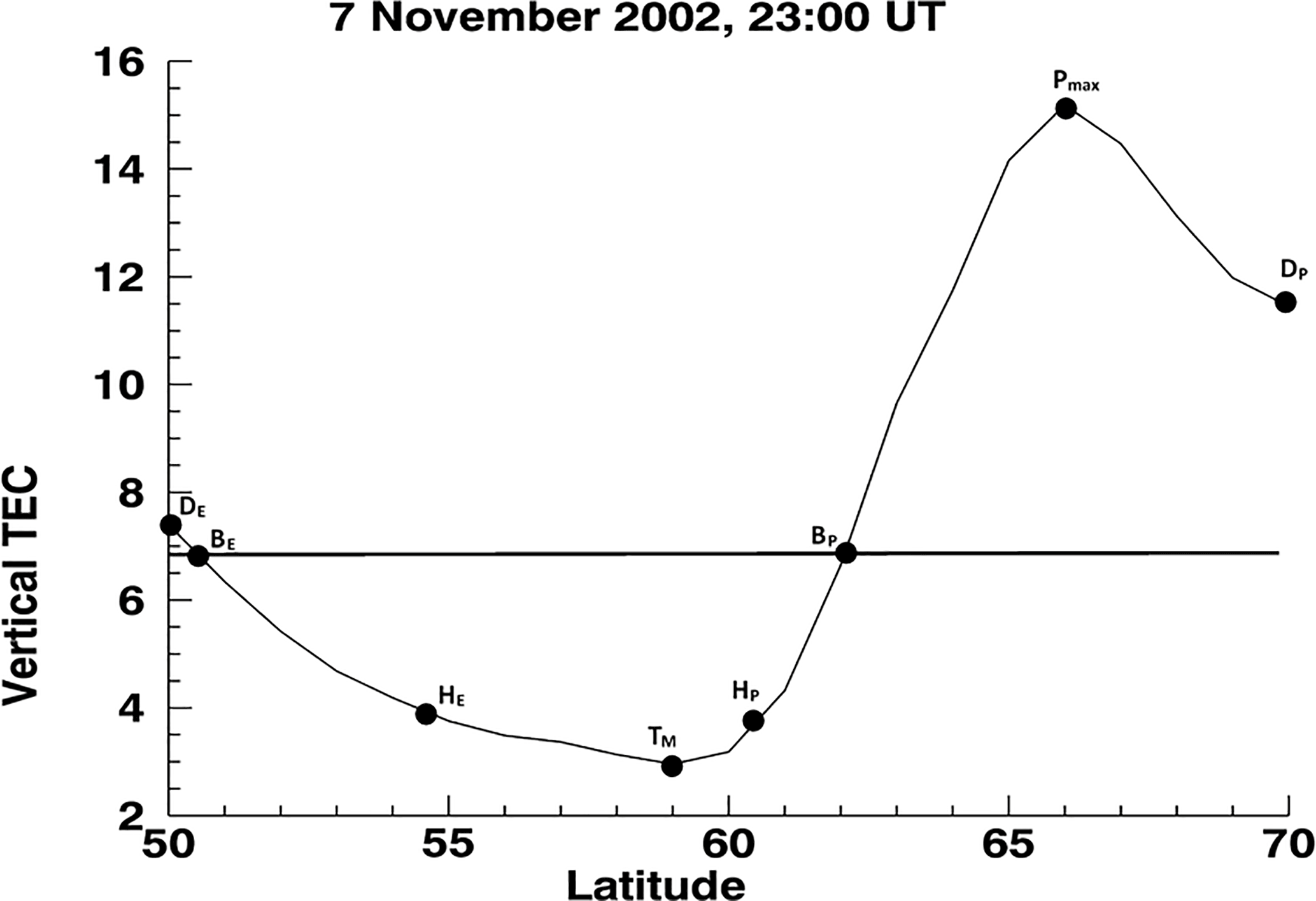
Figure 2Example plot, for 23:00 UT on 7 November 2002, of VTEC (in TECU) at a longitude of 0.0∘ E for the EDAM electron density grid as a function of latitude (in degrees). It illustrates the set of parameters used to characterize the location and shape of the main ionization trough. The horizontal line shows the average TEC over the latitudinal profile, and breakpoints are identified where this average level intersects the profile. The trough is characterized by the following parameters: the trough minimum (TM), equatorward extreme (DE), poleward extreme (DP), equatorward breakpoint (BE), poleward breakpoint (BP), equatorward half point (HE), the poleward half point (HP) and the poleward maximum (Pmax). The half points are used to characterize the shape of the trough in the vicinity of the trough minimum.
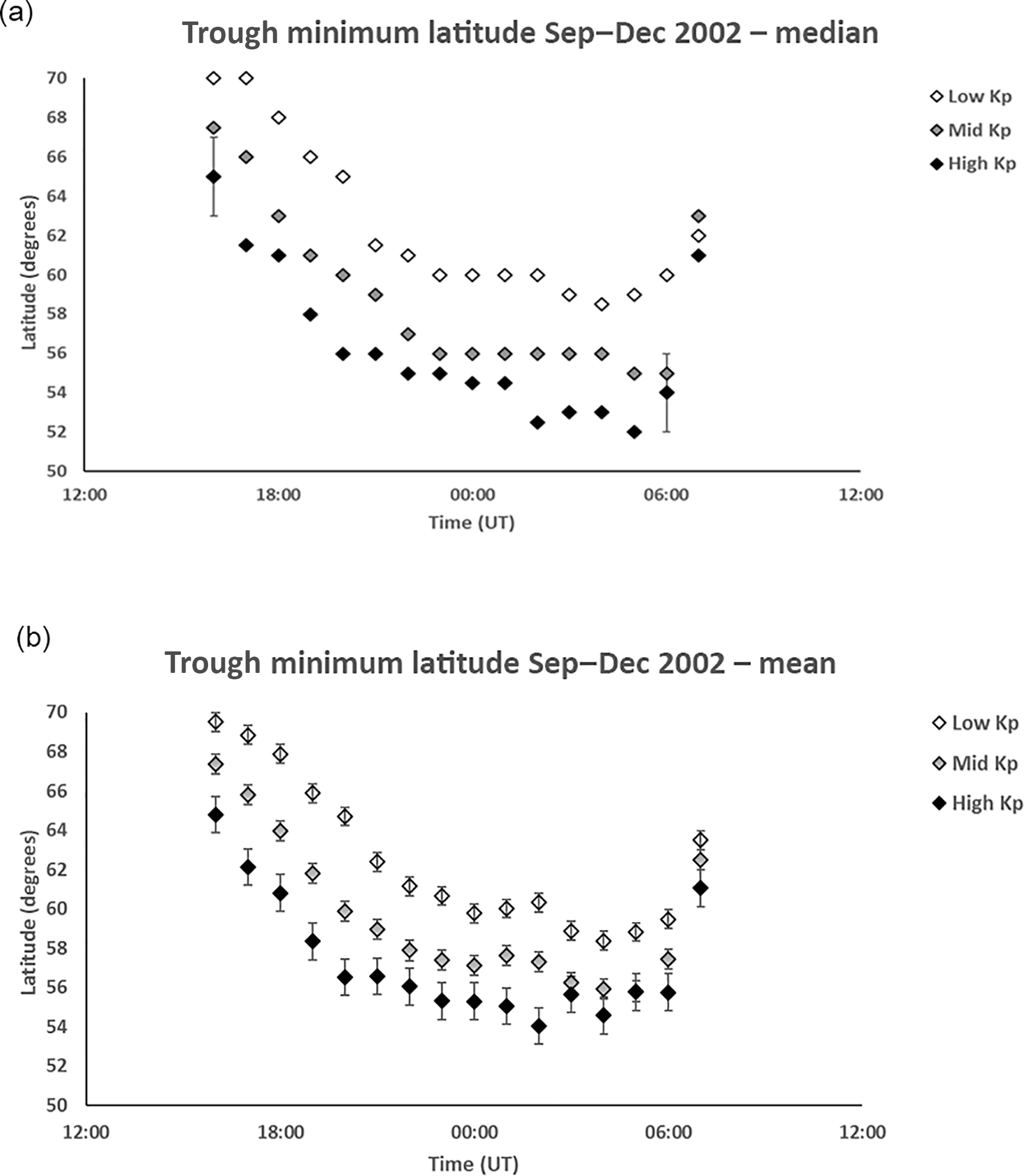
Figure 3(a) Median latitudes for the trough minimum from 16:00 to 07:00 UT for low Kp (0 to 2+), medium (“Mid”) Kp (3− to 4) and high Kp (≥ 4+). The representative interquartile range shown on two points is approximately 4.0∘ latitude. The trough minimum occurs at the highest latitudes in early evening and moves progressively equatorward with increasing time before retreating rapidly poleward near 07:00 UT. (b) Mean latitudes for the trough minimum from 16:00 to 07:00 UT for low Kp (0 to 2+), medium Kp (3− to 4) and high Kp (≥ 4+). The bars show the standard error in the mean for each point. The trends in the plot are the same as for the median values in Fig. 3a.
Figure 3b shows the corresponding plot for the mean latitudes of the trough minimum. In this case the bars show the standard error in the mean. The sequences of points show the same trends as for the median values, although with slight differences with the minimum values at high geomagnetic activity reaching 54–56∘ N between 02:00 and 05:00 UT, which is a higher latitude than that for the median values.
The median and mean VTEC values at the trough minimum are shown in Fig. 4a and b, respectively. The representative interquartile range for the median plot was approximately 2.5 TECU and the standard error in the mean for each mean value are indicated by the bars in the second figure. Figure 4a shows that the earlier VTEC are larger for the most active geomagnetic activity, being in excess of 12 TECU at 16:00 UT. At times, beyond 21:00 and until 05:00 UT, the median values for the low Kp range tend to be less than 4 TECU, although there is no clear difference between the values for the three ranges of geomagnetic activity in this region given the overlap of the interquartile ranges. A similar trend is seen in the mean values. The effect of increased ionization production at dawn again starts to be evident at 06:00 UT in these figures and is clear by 07:00 UT.
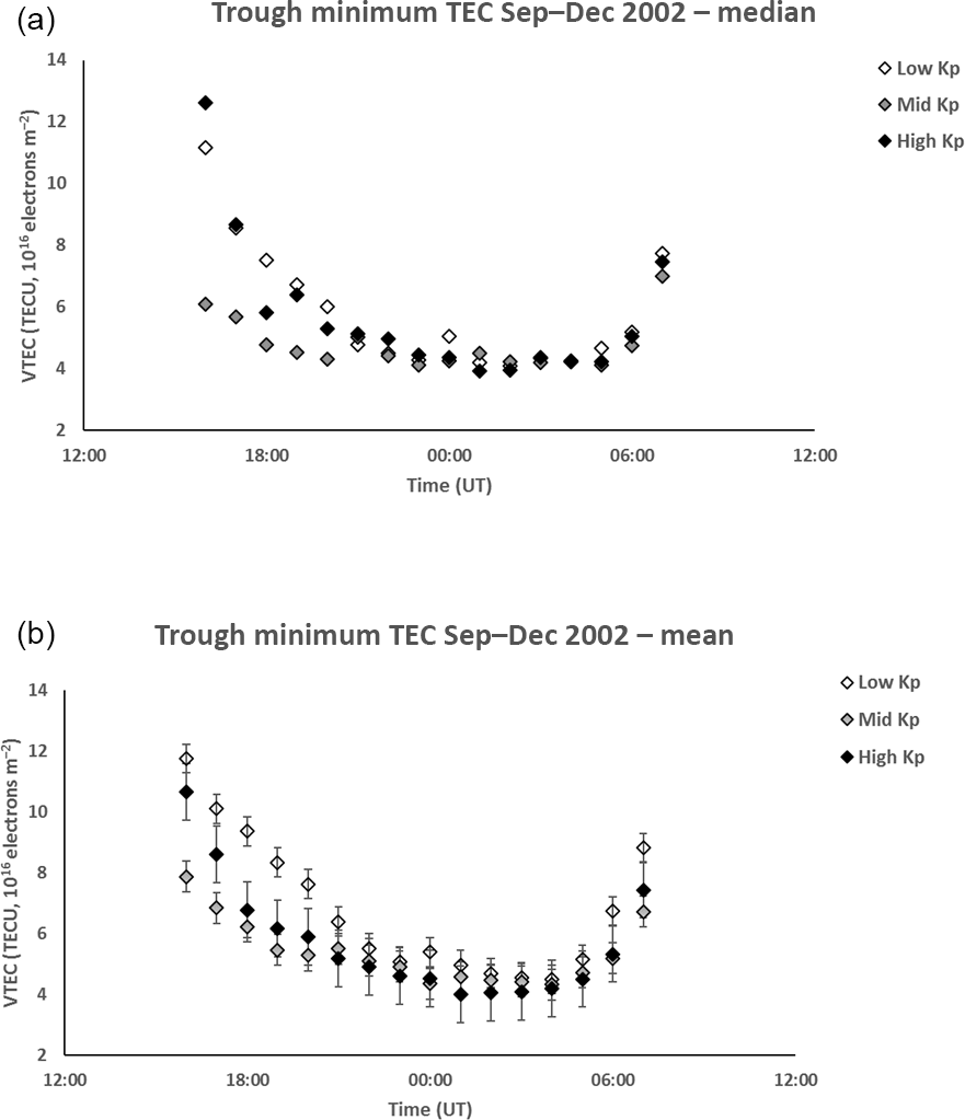
Figure 4(a) Median VTEC for the trough minimum from 16:00 to 07:00 UT for low Kp (0 to 2+), medium Kp (3− to 4) and high Kp (≥ 4+). The representative interquartile range is approximately 2.5 TECU. Between 21:00 and 07:00 UT there is no clear difference between the values for the three ranges of geomagnetic activity. (b) Mean VTEC for the trough minimum from 16:00 to 07:00 UT for low Kp (0 to 2+), medium Kp (3− to 4) and high Kp (≥ 4+). The bars show the standard error in the mean for each point. Similarly to Fig. 4a, there is no clear difference in the VTEC between the three levels of geomagnetic activity from 21:00 to 07:00 UT.
Median and mean values were also considered for other parameters; but given the similar trends observed in the two values, only the median values are shown for these. Consideration of the median values reduces potential effects of outliers in the presented data. Figure 5 shows median trough widths, defined as the latitudinal range between the two break points (BP and BE). For most of the night the width is largest for the lowest Kp range, being between 11 and 13∘ after 21:00 UT. Distinguishing between the other two Kp ranges is not so clear, with both tending to show variable widths of between 9 and 11∘ latitude with lowest values occurring between 23:00 and 04:00 UT.
Figure 6 shows the median trough depth, defined as the difference between the average VTEC of the profile (VTEC at the breakpoint) and its value at the trough minimum. There is no clear dependency on Kp, with each activity range showing values below 4 TECU from 18:00 UT and reaching consistently lower values of 2 TECU or less from about 03:00 UT.
Evidence of asymmetry in the trough shape is seen in the equatorward and poleward half-width of the trough (Fig. 7a and b respectively). These are the widths from the equatorward breakpoint to the trough minimum and from the minimum to the poleward breakpoint. Median values for the equatorward half-width are generally between 4 and 8∘ in latitude with those for the lowest geomagnetic activity tending to be largest until about 02:00 UT. Values for the poleward half-width are generally between about 4 and 6∘ latitude. The width tends to be largest for the highest Kp range. The suggestion here is that geomagnetic activity affects both the equatorward and poleward sides of the trough.
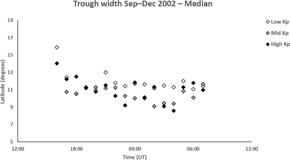
Figure 5Median trough widths from 16:00 to 07:00 UT for low Kp (0 to 2+), medium Kp (3− to 4) and high Kp (≥ 4+). The representative interquartile range is approximately 2.5∘ latitude. Between 21:00 and 04:00 UT, the trough width, of 11–13∘ latitude, for the low Kp is generally larger than for the other geomagnetic activity series.

Figure 6Median trough depth from 16:00 to 07:00 UT for low Kp (0 to 2+), medium Kp (3− to 4) and high Kp (≥ 4+). The representative interquartile range is approximately 1.5 TECU. There is no clear dependency of the trough depth on geomagnetic activity.
The median gradient of the equatorward trough wall taken from the trough minimum to the break point is at its steepest at earlier times with the initial values being more than 1 TECU per degree latitude (Fig. 8a). It reduces to about 0.2–0.4 TECU per degree latitude from about 22:00 UT and then decreases further before dawn. With the exception of before 22:00 UT, the gradient of the poleward wall (Fig. 8b) tends to be slightly larger than that of the equatorward wall, with values generally between 0.3 and 0.6 TECU per degree latitude but reducing in the pre-dawn hours. It is interesting that both gradients show a hint of increased values near midnight, for the medium geomagnetic range.
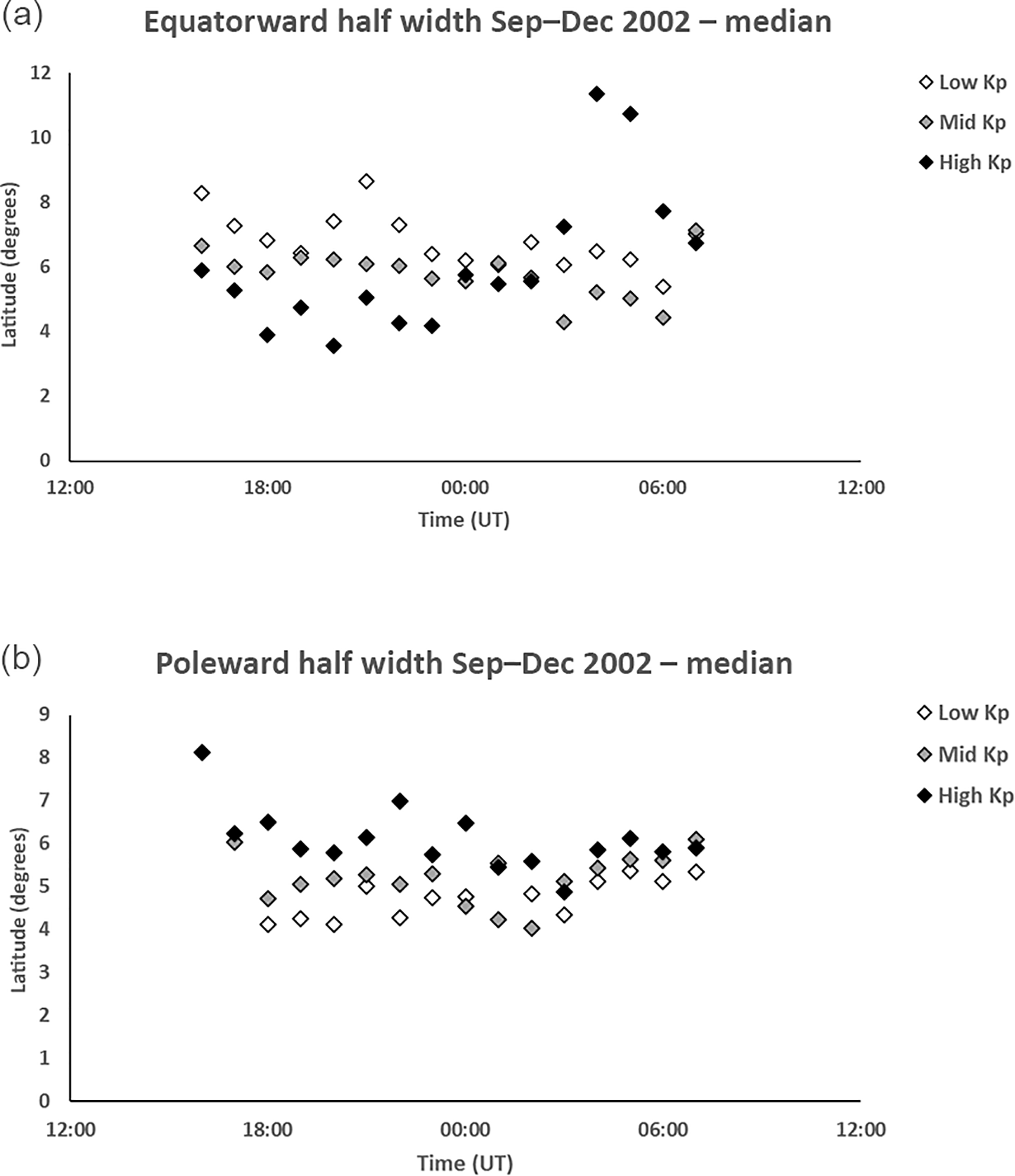
Figure 7(a) Median equatorward half-width of the trough from 16:00 to 07:00 UT for low Kp (0 to 2+), medium Kp (3− to 4) and high Kp (≥ 4+). The representative interquartile range is approximately 3.0∘ latitude. The equatorward half-width prior to 04:00 UT is generally largest for the low Kp level and smallest for the the high Kp level. (b) Median poleward half-width of the trough from 16:00 to 07:00 UT for low Kp (0 to 2+), medium Kp (3− to 4) and high Kp (≥ 4+). The representative interquartile range is approximately 2.5∘ latitude. In contrast to Fig. 7a, the poleward widths tend to be largest for the high Kp levels and smallest for the low Kp levels.
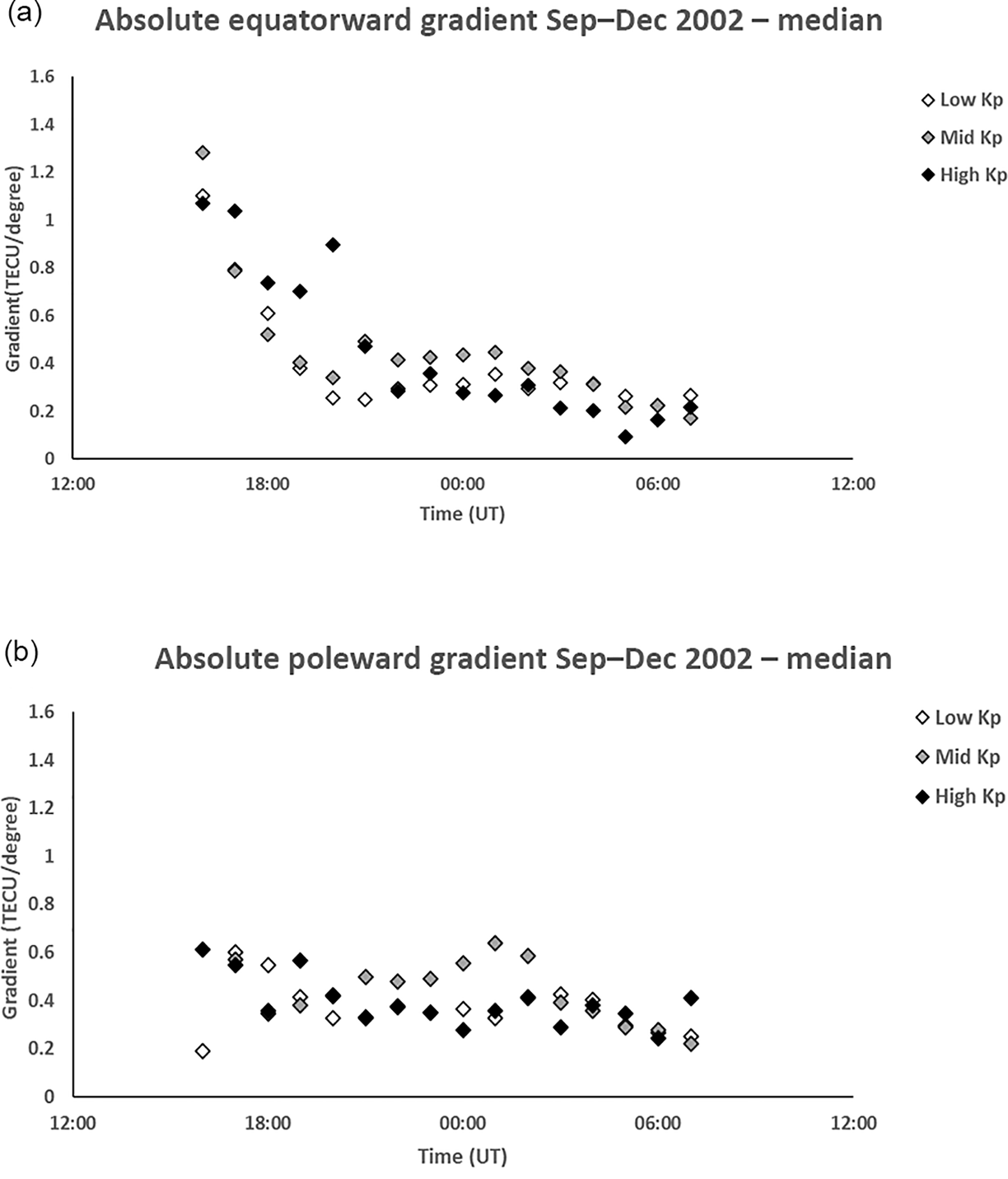
Figure 8(a) Median gradient of the equatorward wall of the trough from 16:00 to 07:00 UT for low Kp (0 to 2+), medium Kp (3− to 4) and high Kp (≥ 4+). The representative interquartile range is approximately 0.25 TECU per degree. The gradient declines as the night progresses from in excess of 1.0 TECU per degree in early evening to less than 0.4 TECU per degree after about 21:00 UT. (b) Median gradient of the poleward wall of the trough from 16:00 to 07:00 UT for low Kp (0 to 2+), medium Kp (3− to 4) and high Kp (≥ 4+). The representative interquartile range is approximately 0.3 TECU per degree. The gradient is generally between 0.3 and 0.6 TECU per degree throughout the night.
Figure 9a and b show the median latitude of the maximum VTEC on the poleward side of the trough and the maximum VTEC of the feature, respectively. Caution is needed up to about 18:00 UT owing to a small number of data values, with the feature likely to have been poleward of the field-of-view. The median latitude is generally at higher latitudes for the lowest Kp range between 21:00 and 05:00 UT, being at about 68∘ N in the pre-midnight sector and moving to about 66∘ N in the post-midnight sector (Fig. 9a). The latitude tends to be at about 64∘ N for the high Kp range in the post-midnight sector but increases near dawn. The maximum VTEC shows a general decrease during the course of the night, but there is no clear dependency on geomagnetic activity (Fig. 9b).
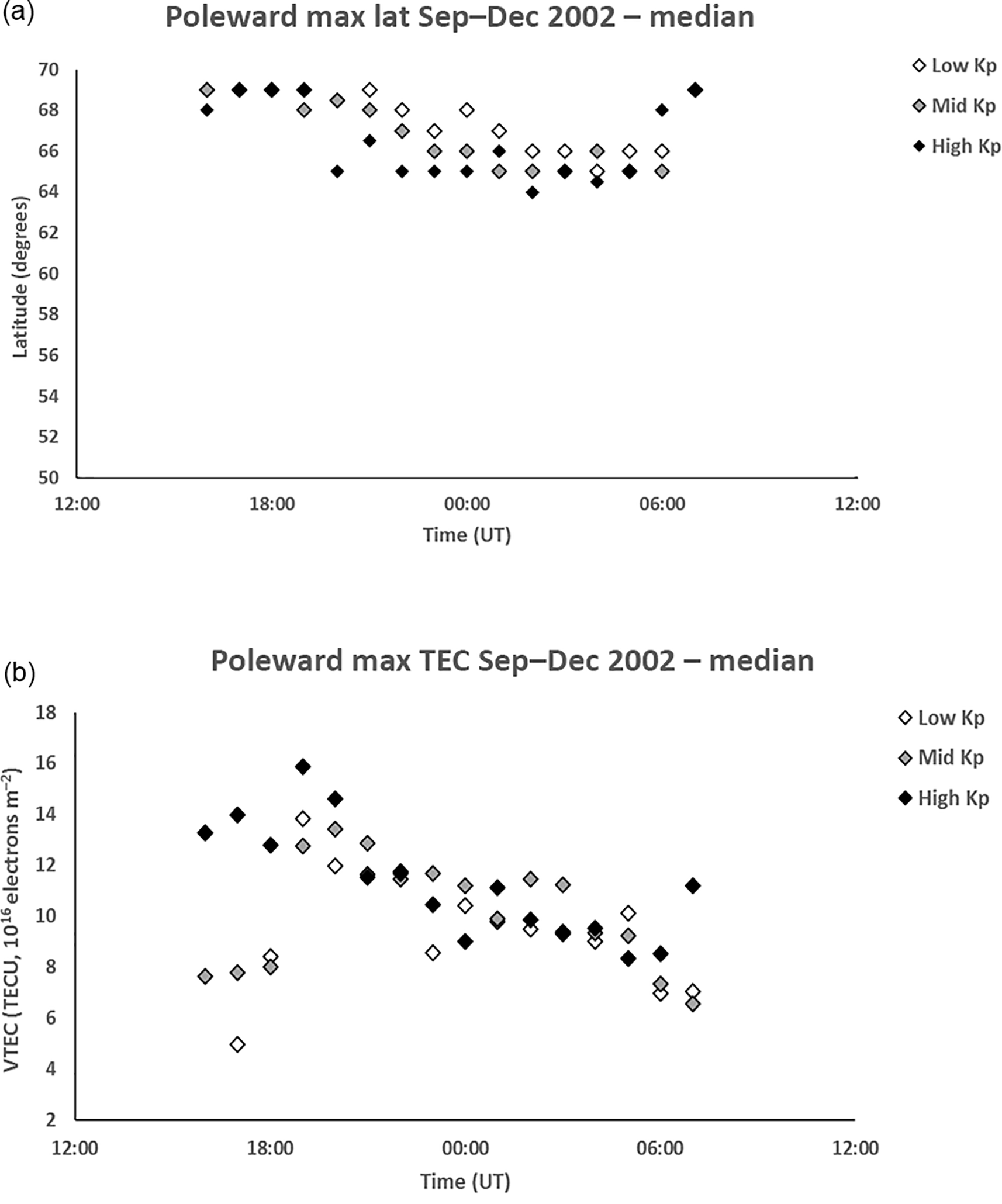
Figure 9(a) Median latitude of the maximum VTEC on the poleward side of the trough from 16:00 to 07:00 UT for low Kp (0 to 2+), medium Kp (3− to 4) and high Kp (≥ 4+). The representative interquartile range is approximately 2.0∘. The poleward maximum moves equatorward during the course of the night, with the location for the high geomagnetic activity being at the lowest latitudes but increasing near dawn. (b) Median of the maximum VTEC on the poleward side of the trough from 16:00 to 07:00 UT for low Kp (0 to 2+), medium Kp (3− to 4) and high Kp (≥ 4+). The representative interquartile range is approximately 5.0 TECU. The VTEC decreases from in excess of 12 TECU at 19:00 UT to about 8 TECU at 06:00 UT.
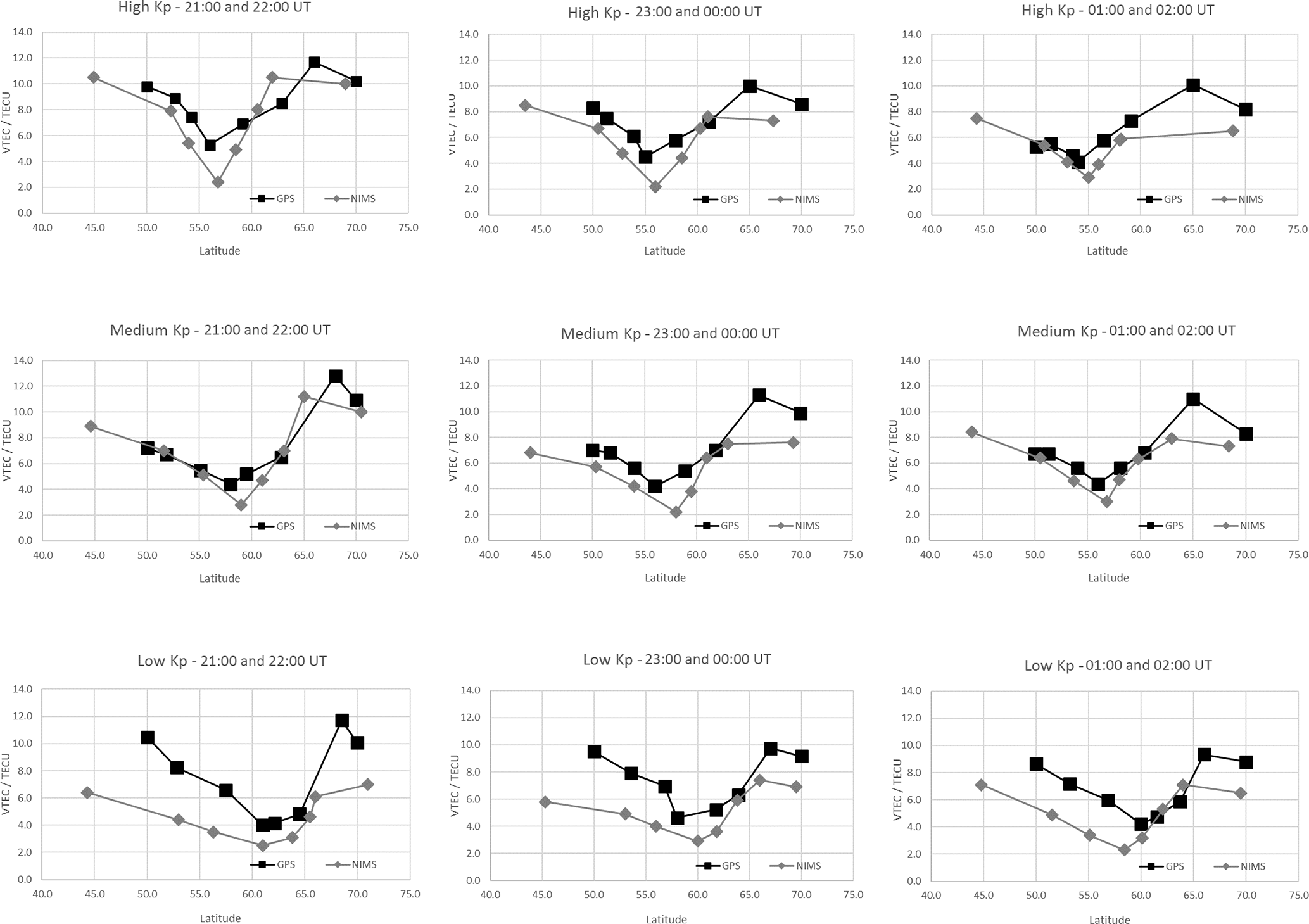
Figure 10Parameterization profiles from the EDAM model with GPS assimilated data (black) for low Kp (0 to 2+), medium Kp (3− to 4) and high Kp (≥ 4+) and for the NIMS tomography observations (grey) from Pryse et al. (2006) for low Kp (0 to 2+), medium Kp (3− to 4−) and high Kp (4 to 7+). The points show the median values for DE (equatorward extreme), BE (equatorward breakpoint), HE (equatorward half point), TM (trough minimum), HP (poleward half point), BP (poleward break point), Pmax (maximum on poleward side of the trough) and DP (poleward extreme) for three time bins. For EDAM, these were for the combined hourly values of 21:00 and 22:00, 23:00 and 00:00, and 01:00 and 02:00 UT indicated on the panels. The corresponding time intervals for NIMS were 21:00 to almost 23:00, 23:00 to almost 01:00, and 01:00 to almost 03:00 UT.
Table 1(a) Latitude (in degrees north) and VTEC (in TECU) of the set of parameters used to characterize the shape of the trough obtained from the EDAM model for low geomagnetic activity, Kp (0 to 2+). (b) Latitude (in degrees north) and VTEC (in TECU) of the set of parameters used to characterize the shape of the trough obtained from the EDAM model for medium geomagnetic activity, Kp (3− to 4). (c) Latitude (in degrees north) and VTEC (in TECU) of the set of parameters used to characterize the shape of the trough obtained from the EDAM model for high geomagnetic activity, Kp (≥ 4+).
Figure 10 shows a comparison of the main trough in terms of the defined parameters from the NIMS tomography observations and the current EDAM/GPS modelling. The trough is represented by the median values of the trough parameters for DE (equatorward extreme), BE (equatorward breakpoint), HE (equatorward half point), TM (trough minimum), HP (poleward half point), BP (poleward break point), Pmax (maximum VTEC on the poleward side of the trough) and DP (poleward extreme). The parameters are shown for three time intervals. For EDAM, these were for latitudinal profiles at 21:00 and 22:00 UT that were combined into one bin, similarly for profiles at 23:00 and 00:00 UT that were combined into a second bin, and profiles at 01:00 and 02:00 UT combined into a third bin. For the NIMS observations in the earlier paper, the closest corresponding bins were for satellite passes monitored in bins 21:00 to almost 23:00 UT, 23:00 to almost 01:00 UT, and 01:00 to almost 03:00 UT. The three levels of geomagnetic activity were considered. For the EDAM data, these levels were low Kp (0 to 2+), medium Kp (3− to 4) and high Kp (≥ 4+). The boundaries of medium and high Kp were slightly different for the NIMS data with medium Kp (3− to 4−) and high Kp (4 to 7+). Comparison with low Kp shows good agreement, with the GPS VTEC values being marginally larger than the NIMS values. In both cases the curves show an asymmetry in a wide trough under low geomagnetic conditions with an equatorward wall of smaller gradient than that of the poleward wall. The NIMS results show a clear indication of the boundary blob. It is likely that the EDAM model is not so able to resolve the signatures of this latitudinally confined ionization blob with sharp gradients on either side. In general, the EDAM trough values are consistently higher than those of the NIMS with a difference of up to 2 TECU, although it is markedly larger at the equatorward latitudes under quiet geomagnetic conditions. This difference is likely to be the consequence of the altitude of the satellites, with the long path lengths from satellite to receiver in the EDAM cases traversing topside ionization, while the paths from the lower NIMS satellites do not. There is also some evidence of the equatorward wall becoming steeper as the geomagnetic activity increases in the pre-midnight sector.
For completeness, and in line with the earlier study, the values of the parameters describing the shape of the trough obtained from the EDAM modelling are given in Table 1a–c for low, medium and high geomagnetic activity levels, respectively.
The trends in the trough behaviour modelled by EDAM show general agreement with the earlier study of Pryse et al. (2006). The TEC observations in both the current and earlier study were made using differential carrier phase observations of coherent radio transmissions from satellites. However, there were also significant differences. The earlier study used the VHF and UHF signals from the low Earth orbiting NIMS satellites received at four ground stations, with tomographic reconstruction of the measured TEC providing an image of the ionosphere over a latitude versus height grid during the 20 min duration of each satellite pass. The VTEC was calculated from these images. The current study obtained the TEC by using L-band transmissions from the GPS satellites at the much higher altitudes of about 20 200 km. These signals were monitored by a network of 46 ground-based receivers in Europe, with data from at least 39 receivers assimilated into EDAM at any one time to give the temporally evolving electron density over the 3-D model grid. The VTEC was calculated as a function of latitude at the grid cells covering 0.0∘ E.
The equatorward motion of the trough minimum during the night at each of the three geomagnetic activity levels (Fig. 3a) was as expected from the study of Pryse et al. (2006). Figure 2a from Pryse et al. (2006) corresponds to Fig. 3a in this current study. Both figures show the trend of the latitude of the trough minimum moving progressively equatorward from 18:00 until 06:00 UT. Both figures also show the effect of geomagnetic activity on the latitude, with the trough minimum at the lowest latitudes under high levels of Kp. In the current study, the lowest latitudes reached by the trough in pre-dawn hours were approximately 52, 55 and 58∘ N for the low, medium and high Kp bands, respectively. The difference of about 6∘ latitude between quiet and active geomagnetic activity can be compared with other earlier studies. Lee et al. (2011) report an equatorward shift of about 3–5∘ latitude for the trough minimum with increased geomagnetic activity in their study, while Fig. 3 of the statistical study of Yang et al. (2015) shows a consistent decrease in magnetic latitude from low to high Kp values. In such comparisons, it is important to appreciate that different observing techniques have been used and during different times in the solar cycle. For example, Lee et al. (2011) used radio occultation to infer NmF2, while the current study uses the assimilation of slant TEC into EDAM to give the VTEC.
The VTEC values of the trough minimum did not show a clear dependence on geomagnetic activity (Fig. 4), in keeping with the earlier study of Pryse et al. (2006). However, the minimum value in the current study was 4 TECU compared to the 2 to 3 TECU in the previous study. It is likely that the difference is attributed to the TEC observations, with the GPS observations being from the ground to the satellite altitudes of about 20 200 km, whilst those for the NIMS satellites were merely to an altitude of about 1100 km with the paths not traversing the high protonosphere. Electron densities at altitudes from 750 to 2000 km at 250 km altitude increments given by IRI2007 at 21:00, 00:00 and 03:00 UT on 20 October 2002 at 60∘ N were considered. For each time, and assuming an exponential decrease in electron density with height in this altitude range, a decay constant was determined. Applying this decay to altitudes from 1000 km to the altitude of GPS at approximately 20 200 km gave TECs between 1000 km and the GPS altitude of 0.6, 0.6 and 0.4 TECU for 21:00, 00:00 and 03:00 UT, respectively. While the decrease in electron density may not necessarily conform to the exponential decay, it suggests that TEC in the high topside ionosphere contributes some 10 % to the EDAM TEC values. Lunt et al. (1999) observed an average TEC difference between NIMS and GPS of some 1.6 TECU at 50.4∘ N, reducing to 0.75 TECU at 51.4∘ N and to about 0.05 TECU at 52.4∘ N at solar minimum. Yang et al. (2015) also report an essentially constant TEC at the trough minimum of about 4–5 TECU regardless of Kp, and indicate that investigation of the TEC and temperature at the trough minimum is needed to help with understanding the physical processes responsible for trough formation. When they categorized the data by season, a small decrease in TEC was observed at the trough minimum with MLT at summer and equinox. This reduction was attributed to a loss mechanism such as chemical recombination. Lee et al. (2011) considering NmF2 found that its values at the trough minimum were slightly larger under disturbed conditions than under quiet conditions.
The scatter in the latitudinal width of the trough, defined as the latitudinal range between the two break points (BE and BP), was large in the current investigation ranging from about 9 to 13∘ latitude (Fig. 5), but somewhat smaller than the earlier study of Pryse et al. (2006). The largest width of some 11–13∘ latitude tended to occur under low geomagnetic conditions after about 21:00 UT, with the width for the medium and higher geomagnetic activity at these times being between about 9 and 12∘. The large scatter of width may arise due to variability in auroral activity. Zou et al. (2011) investigated the effect of substorms on the trough width in the Alaskan sector, reporting a rapid equatorward movement of the poleward trough wall at substorm onset with a narrowing of the trough and sometimes its disappearance. The trough then expanded back to the higher latitudes at substorm recovery as the auroral region retreated poleward.
The current study showed that the trough depth, from the level of the breakpoints to the trough minimum, for all bands of Kp tended to group together from about 18:00 UT with median values of about 2–3 TECU (Fig. 6) with the scatter in the values reducing with increasing UT. At earlier times the values were larger, with those at low geomagnetic activity tending to be largest. Values decreased below 2 TECU after about 03:00 UT with further reduction in scatter. There is a suggestion of a larger spread of trough depths in the pre-midnight hours than at post-midnight. In the earlier paper of Pryse et al. (2006), reference was made to the different physical processes responsible for the formation of the trough in the pre- and post-midnight sectors, and it may be that the different characteristics observed in the current study are also attributed to this. The pre-midnight trough often occurs in the vicinity of slow plasma drift at the interface between the westward flow at the poleward side of the dusk convection cell and the counter eastward co-rotating motion on the equatorward side (Spiro et al., 1978). After the Harang discontinuity near local magnetic midnight the trough may be a fossil from the earlier time in the eastward flow in the dawn sector as mentioned by Pryse et al. (2006), although the continuing decrease evident after 03:00 UT may be attributed to continuing chemical loss (Lee et al., 2011). The statistical study of He et al. (2011) considered NmF2 for magnetic activity Kp of less than 3 and categorized the data by season and hemisphere. They concluded that the depth of the midnight trough showed longitudinal dependency in the equinox seasons and summer, and related this to the neutral winds and the configuration of the geomagnetic field.
The larger equatorward half-width, measured from the trough minimum to the equatorward breakpoint near midnight for the lowest Kp range (Fig. 7a), is in keeping with the narrower equatorward half-width at highest Kp levels in the earlier study, although there is substantial scatter in this equatorward parameter. As in the earlier study, it was rather unexpected that processes on the equatorward side of the trough may be affected by geomagnetic activity.
The current study showed a poleward half-width with some larger values near midnight under disturbed geomagnetic activity (Fig. 7b), but as in the previous study the scatter was smaller than that for the equatorward half-width. The results suggest an asymmetry in the trough width with that under lower geomagnetic activity having the larger equatorward half-width and smaller poleward half-width and that under higher geomagnetic activity having the larger poleward half-width and smaller equatorward half-width. Further study of the physical processes operative in the trough are needed to reconcile these observations with those of Zou et al. (2011), where the substorm activity rapidly moves the poleward trough wall equatorward.
As in Pryse et al. (2006), there was evidence of a decreasing gradient for the equatorward wall during pre-midnight hours (Fig. 8a). The general decrease continues to later times but decreasing at a smaller rate to a level of some 0.2 TECU per degree. Near midnight there is some evidence that the moderate geomagnetic data have the steeper gradient. There is no clear reason for this, but interestingly a similar observation is seen for the poleward wall gradient shortly after midnight in the EDAM VTEC (Fig. 8b) and likewise in the NIMS poleward gradient values.
Under quiet geomagnetic conditions the boundary blob on the poleward side of the trough moves equatorward near midnight (Fig. 9a). There is also evidence of this at the more active geomagnetic levels, but it is clear that the blob maximum is generally at lower latitudes under these more disturbed conditions. The maximum VTEC decreases during the course of the night for each level of geomagnetic activity (Fig. 9b).
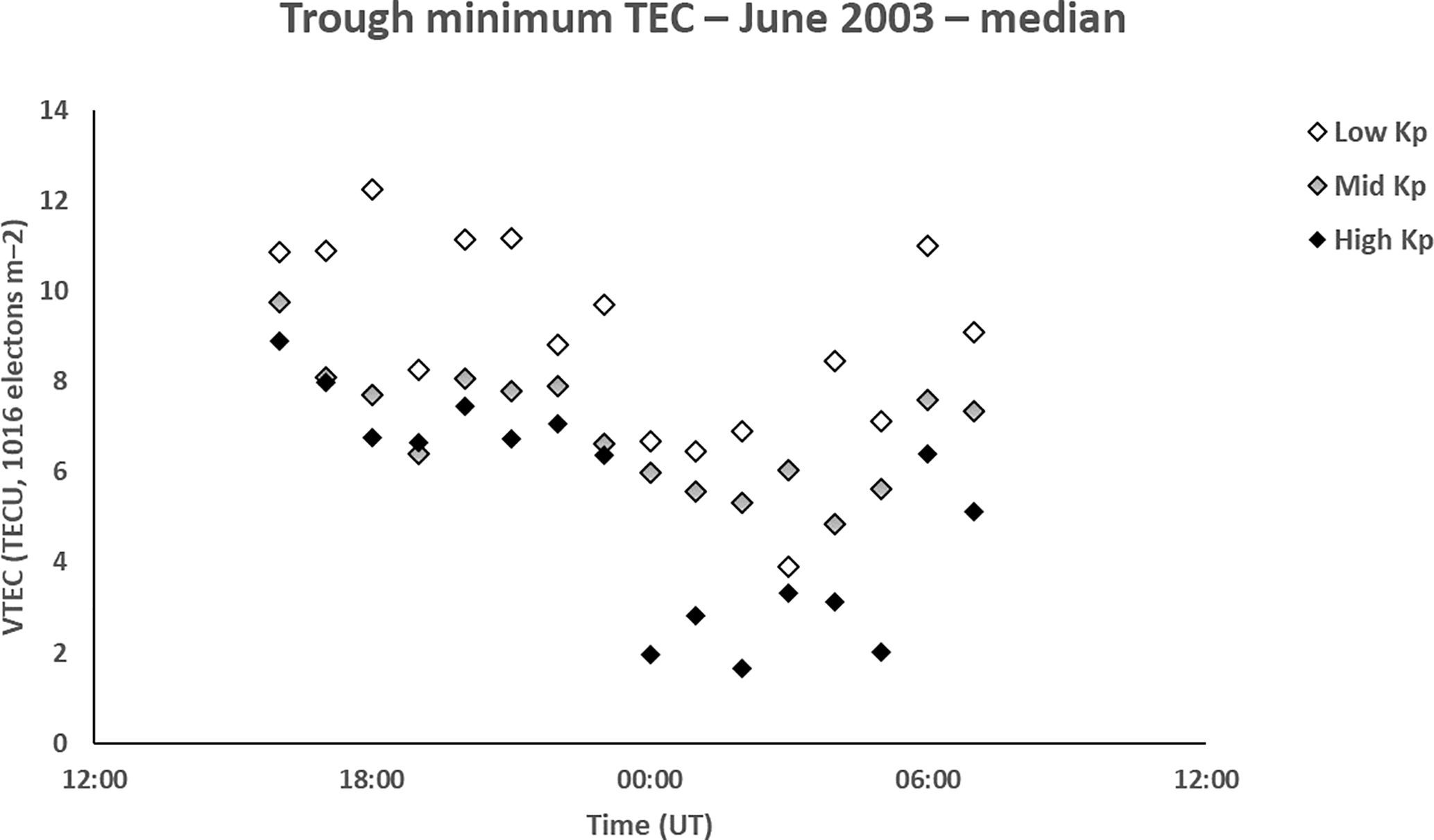
Figure 11Median VTEC for the trough minimum in June 2003 from 16:00 to 07:00 UT for low Kp (0 to 2+), medium Kp (3− to 4) and high Kp (≥ 4+). The representative interquartile range is approximately 2.5 TECU. The VTEC values are clearly larger than for the prominent trough considered for the main study, apart from between 00:00 and 05:00 UT for high Kp.
In summary, there is general agreement and consistency between the observations of the trough in the current study and those of the earlier reported observations, despite significant differences in the techniques. This broad agreement gives support for the application of EDAM with the assimilation of GPS TEC to model the mid-latitude trough. It reinforces the use of EDAM for monitoring the ionospheric trough, and indeed to model other ionospheric features with latitudinal gradients on similar scales. Given the global coverage of the constellation of GPS satellites and the network of ground receivers, it opens up the possibility of global monitoring of such features with large-scale latitudinal gradients, and also for the use of the technique in scientific studies.
The current study has considered periods when troughs were prominent, so that they were in keeping with the troughs considered in the earlier study. Summertime troughs were therefore not considered. Figure 11 shows the median TEC at the trough minimum for June 2003 for the three categories of geomagnetic activity. With the exception of 00:00–05:00 UT under conditions of high Kp, all TEC values are larger than those obtained in the main study for September to December 2002, in keeping with increased solar illumination in June. They also show substantially more variability than for the current study. Some caution is needed in the interpretation of the high Kp values as the performance of the EDAM was reduced under the disturbed conditions for this month. The differences in the summertime troughs in comparison with those at the equinox and winter provides evidence for seasonal variability in the trough modelled by EDAM. This is not the main focus of this current paper and will not be considered further here. However, the validation of the ability of EDAM to model the trough and other features with steep gradients covered in this paper, and the vast database of GPS observations, opens up the possibility of broader statistical studies of ionospheric large-scale structure. The current study has considered data from 2002, specifically for comparison with the earlier results. However, for future studies, a larger database of GPS data is available from more recent years. Comparisons of the results from such studies of seasonal variation in the European sector with studies such as that reported by Le et al. (2017) in the North American sector (60.0 to 90.0∘ W) have the potential of addressing physical processes operating in the trough region, in particular because of the differences in the geographic/geomagnetic latitudes relation in the two sectors, and may give indication of the interplay between the roles of solar illumination and geomagnetic influences on the trough behaviour.
Statistical results have been presented of the mid-latitude trough, obtained from the EDAM model with GPS TEC assimilation. Approximately 1950 samples of the trough have been included in the study. The results have not only considered the width and depth of the trough but have also been used to parameterize the trough shape in terms of a set of well-defined parameters. These parameters were used in a previous study that used NIMS TEC measurements and tomographic imaging.
The results showed the expected behaviour of trough latitude, width and depth, together with trough-wall gradients. The median values of the defined trough parameters showed broad agreement with the values obtained in the earlier studies, despite being obtained by a different technique. The TEC trough minimum observed by EDAM with GPS assimilation were generally some 1–2 TECU larger than that at the minimum observed previously by the NIMS tomography observations. This is in line with the higher altitude of the GPS satellites compared to the lower orbiting NIMS satellites, with the satellite-to-ground paths of the GPS observations traversing paths through the topside ionosphere. Whilst the electron density in the topside is expected to be low, taken with the long path lengths it gives a measurable increase in the TEC.
This is the first time that the EDAM model has been used in a comparison of the trough with independent observations. Whilst there are differences between the EDAM results and the earlier observations, including the observing geometry, technique, time period of observations and categorization of the Kp levels, the similarities in the observed trough behaviour and its parameterization are encouraging. This provides support for the use of EDAM for modelling the mid-latitude trough. It also provides evidence for the ability of EDAM to model large-scale structure in the ionosphere. Whilst the technique is unlikely, in its present form, to reveal latitudinally narrow structures on scales of typically 1–2∘, such as the boundary blob, it provides convincing evidence of the ability to model features on the scale of the mid-latitude trough and its poleward and equatorward walls covering ∼ 10∘ latitude.
Given the global coverage of the EDAM model and the GPS observations, they show the potential of the technique to image large-scale latitudinal features on a global basis, provided there is a sufficient density of ground receivers. It opens the possibility for using the technique for statistical studies of such features and their dependencies on, for example, season, geomagnetic and solar conditions.
The sources for data used in this study have been mentioned in the acknowledgments of the paper.
JADP carried out the collection and statistical analysis of the data set with the guidance of SEP. NJB aided with the model and data collection program. All authors contributed with the compiling of the manuscript.
The authors declare that they have no conflict of interest.
James A. D. Parker acknowledges QinetiQ for providing the model and
assistance in producing these results for his studies. Use of the NASA CDDIS
archive for the GPS data of the International GNNS service is also gratefully
acknowledged (https://cddis.nasa.gov/). The Kp indices were obtained
via the UKSDDC website,
https://www.ukssdc.ac.uk/data_menu.html.
The topical
editor, Ana G. Elias, thanks two anonymous referees for help in evaluating
this paper.
Andreev, M. Yu., Lukicheva, T. N., and Mingalev, V. S.: Model study of the effect of the main ionospheric trough on oblique HF radiowave propagation, Geomagn. Aerononmy, 46, 94–100, 2006.
Angling, M. J. and Cannon, P. S.: Assimilation of radio occultation measurements into background ionospheric models, Radio Sci., 39, RS1S08, https://doi.org/10.1029/2002RS002819, 2004.
Angling, M. J. and Jackson-Booth, N. K.: A short note on the assimilation of collocated and concurrent GPS and ionosonde data into the Electron Density Assimilative Model, Radio Sci., 46, RS0D13, https://doi.org/10.1029/2010RS004566, 2011.
Angling, M. J. and Khattatov, B.: Comparative study of two assimilative models of the ionosphere, Radio Sci., 41, RS5S20, https://doi.org/10.1029/2005RS003372, 2006.
Bates, H. F., Belon, A. E., and Hunsucker, R. D.: Aurora and the poleward edge of the main ionospheric trough, J. Geophys. Res., 78, 648–658, https://doi.org/10.1029/JA078i004p00648, 1973.
Bilitza, D., Reinisch, B. W., Radicella, S. M., Pulinets, S., Gulyaeva, T., and Triskova, L.: Improvements of the International Reference Ionosphere model for the topside electron density profile, Radio Sci., 41, RS5S15, https://doi.org/10.1029/2005RS003370, 2006.
Crowley, G.: Critical Review of Ionospheric Patches and Blobs, Review of Radio Science 1993–1996, edited by: Ross Stone, W., 619–648, URSI, Oxford University Press, 1996.
Feichter, E. and Leitinger, R.: Properties of the main trough of the F region derived from Dynamic Explorer 2 data, Ann. Geophys., 45, 117–124, https://doi.org/10.4401/ag-3491, 2002.
Feltens, J., Angling, M., Jackson-Booth, N., Jakowski, N., Hoque, M., Hernández-Pajares, M., Aragón-Àngel, A., Orús, R., and Zandbergen, R.: Comparative testing of four ionospheric models driven with GPS measurements, Radio Sci., 46, RS0D12, https://doi.org/10.1029/2010RS004584, 2011.
He, M., Liu, L., Wan, W., and Zhao, B.: A study on the nighttime midlatitude ionospheric trough, J. Geophys. Res., 116, A05315, https://doi.org/10.1029/2010JA016252, 2011.
Hedin, M., Häggström, I., Pellinen-Wannberg, A., Andersson, L., Brändström, U., Gustavsson, B., Steen, Å., Westman, A., Wannberg, G., Eyken, T. V., Aso, T., Cattell, C., Carlson, C. W., and Klumpar, D.: 3-D extent of the main ionospheric trough – a case study, Adv. Polar Upper Atmos. Res., 14, 157–162, 2000.
Hochegger, G., Nava, B., Radicella, S., and Leitinger, R., A family of ionospheric models for different uses, Phys. Chem. Earth, Pt. C, 25, 307–310, https://doi.org/10.1016/S1464-1917(00)00022-2, 2000.
Hofmann-Wellenhof, B., Lichtenegger, H., and Collins, J.: GPS Theory and Practice, 5th Edn., Springer-Verlag, Wien, New York, 2000.
Horvath, I. and Crozier, S.: Software developed for obtaining GPS-derived total electron content values, Radio Sci., 42, RS2002, https://doi.org/10.1029/2006RS003452, 2007.
Ishida, T., Ogawa, Y., Kadokura, A., Hiraki, Y., and Häggström, I.: Seasonal variation and solar activity dependence of the quiet-time ionospheric trough, J. Geophys. Res.-Space, 119, 6774–6783, https://doi.org/10.1002/2014JA019996, 2014.
Jayawardena, T. S. P., Chartier, A. T., Spencer, P., and Mitchell, C. N.: Imaging the topside ionosphere and plasmasphere with ionospheric tomography using COSMIC GPS TEC, J. Geophys. Res.-Space, 121, 817–831, https://doi.org/10.1002/2015JA021561, 2016.
Kersley, L., Pryse, S. E., Walker, I. K., Heaton, J. A. T., Mitchell, C. N., Williams, M. J., and Willson, C. A.: Imaging of electron density troughs by tomographic techniques, Radio Sci., 32, 1607–1621, 1997.
Kersley, L., Malan, D., Pryse, S. E., Cander, L. R., Bamford, R. A., Belehaki, A., Leitinger, R., Radicella, S. M., Mitchell, C. N., and Spencer, P. S. J.: Total electron content: A key parameter in propagation: measurement and use in ionospheric imaging, Ann. Geophys., 47, 1067–1091, 2004.
Krankowski, A., Shagimuratov, I. I., Ephishov, I. I., Krypiak-Gregorczyk, A., and Yakimova, G.: The occurrence of the mid-latitude ionospheric trough in GPS-TEC measurements, Adv. Space Res., 43, 1721–1731, 2009.
Le, H., Yang, N., Liu, L., Chen, Y., and Zhang H.: The latitudinal structure of nighttime ionospheric TEC and its empirical orthogonal functions model over North American sector, J. Geophys. Res.-Space, 122, 963–977, https://doi.org/10.1002/2016JA023361, 2017.
Lee, I. T., Wang, W., Liu, J. Y., Chen, C. Y., and Lin, C. H.: The ionospheric midlatitude trough observed by FORMOSAT-3/COSMIC during solar minimum, J. Geophys. Res., 116, A06311, https://doi.org/10.1029/2010JA015544, 2011.
Lunt, N., Kersley, L., Bishop, G. J., and Mazzella Jr., A. J.: The contribution of the protonosphere to GPS total electron content: Experimental measurements, Radio Sci., 345, 1273–1280, https://doi.org/10.1029/1999RS900016, 1999.
Mitchell, C. N. and Spencer, P. S. J.: A three-dimensional time-dependent algorithm for ionospheric imaging using GPS, Ann. Geophys., 46, 687–696, https://doi.org/10.4401/ag-4373, 2003.
Moffett, R. J. and Quegan, S.: The Mid-Latitude through in the Electron Concentration of the Ionospheric F-Layer: A Review of Observations and Modelling, J. Atmos. Terr. Phys., 45, 315–343, https://doi.org/10.1016/S0021-9169(83)80038-5, 1983.
Muldrew, D. B.: F-layer ionization troughs deduced from Alouette data, J. Geophys. Res., 70, 2635–2650, https://doi.org/10.1029/JZ070i011p02635, 1965.
Pryse, S. E., Kersley, L., Rice, D. L., Russell, C. D., and Walker, I. K.: Tomographic imaging of the ionospheric mid-latitude trough, Ann. Geophys., 11, 144–149, 1993.
Pryse, S. E., Dewis, K. L., Balthazor, R. L., Middleton, H. R., and Denton, M. H.: The dayside high-latitude trough under quiet geomagnetic conditions: Radio tomography and the CTIP model, Ann. Geophys., 23, 1199–1206, https://doi.org/10.5194/angeo-23-1199-2005, 2005.
Pryse, S. E., Kersley, L., Malan, D., and Bishop, G. J.: Parameterization of the main ionospheric trough in the European sector, Radio Sci., 41, RS5S14, https://doi.org/10.1029/2005RS003364, 2006.
Raymund, T. D., Pryse, S. E., Kersley, L., and Heaton, J. A. T.: Tomographic reconstruction of ionospheric electron density with European incoherent scatter radar verification, Radio Sci., 28, 811–817, https://doi.org/10.1029/93RS01102, 1993.
Rodger, A. S., Moffett, R. J., and Quegan, S.: The role of ion drift in the formation of ionization troughs in the mid- and high-latitude ionosphere – a review, J. Atmos. Terr. Phys., 54, 1–30, 1992.
Rycroft, M. J. and Burnell, S. J.: Statistical analysis of movements of the ionospheric trough and the plasmapause, J. Geophys. Res., 75, 5600–5604, https://doi.org/10.1029/JA075i028p05600, 1970.
Spiro, R. W., Heelis, R. A., and Hanson, W. B.: Ion convection and the formation of the mid-latitude F region ionization trough, J. Geophys. Res., 83, 4255–4264, https://doi.org/10.1029/JA083iA09p04255, 1978.
Voiculescu, M., Nygrén, T., Aikio, A., and Kuula, R.: An olden but golden EISCAT observation of a quiet-time ionospheric trough, J. Geophys. Res., 115, A10315, https://doi.org/10.1029/2010JA015557, 2010.
Werner, S. and Prölss, G. W.: The position of the ionospheric trough as a function of local time and magnetic activity, Adv. Space Res., 20, 1717–1722, https://doi.org/10.1016/S0273-1177(97)00578-4, 1997.
Whalen, J. A.: Daytime F Layer Trough Observed on a Macroscopic Scale, J. Geophys. Res., 92, 2571–2576, 1987.
Whalen, J. A.: The daytime F layer trough and its relation to ionospheric-magnetospheric convection, J. Geophys. Res., 94, 17169–17184, 1989.
Yang, N., Le, H., and Liu, L.: Statistical analysis of ionospheric mid-latitude trough over the Northern Hemisphere derived from GPS total electron content data, Earth Planets Space, 196, 201567, https://doi.org/10.1186/s40623-015-0365-1, 2015.
Yeh, K. C. and Raymund, T. D.: Limitations of ionospheric imaging by tomography, Radio Sci., 26, 1361–1380, https://doi.org/10.1029/91RS01873, 1991.
Yizengaw, E. and Moldwin, M. B.: The altitude extension of the mid-latitude trough and its correlation with plasmapause position, Geophys. Res. Lett., 32, L09105, https://doi.org/10.1029/2005GL022854, 2005.
Zou, S., Moldwin, M. B., Coster, A., Lyons, L. R., and Nicolls, M. J.: GPS TEC observations of dynamics of the mid-latitude trough during substorms, Geophys. Res. Lett., 38, L14109, https://doi.org/10.1029/2011GL048178, 2011.