Earth's magnetosheath: a comparison of plasma flow direction between models and observations

Observations of the plasma flow direction in the Earth's magnetosheath are compared with the help of three analytical magnetic-field models, namely Kobel and Flückiger (1994), Romashets and Vandas (2019), and Vandas and Romashets (2019), which all assume current-free fields in the magnetosheath. 47 magnetosheath passages by spacecraft are analyzed in detail and performance of the models are evaluated. It is concluded that the performances measured by mean angles between model and observed flow directions are comparable among the models (the difference of the mean angles is below about 1°), and that they are satisfactory on average (overall mean angles are below 5°). Therefore, a usage of the model by Kobel and Flückiger (1994) is recommended, because it is the simplest one and yields results much faster.

1 Introduction

Earth's magnetic field represents an obstacle for a flowing solar wind (SW). Because the flow is mostly supersonic, a bow shock (BS) is formed ahead. Earth's magnetic field forms a magnetosphere, which is separated from the interplanetary magnetic field (IMF) by a thin layer, the magnetopause (MP). The region between the BS and MP is called the magnetosheath (MSH) and contains compressed, heated, and diverted solar-wind plasma with IMF draped around the MP.

Modeling of the near-Earth environment started soon after the discovery of the SW. First, numerical gasdynamical calculations were performed (Spreiter et al., 1966), followed by MHD simulations intending to include a magnetic field self-consistently (e.g., Spreiter and Stahara, 1980; Siscoe et al., 2002; Samsonov, 2006). Alternatively, there are analytical or semi-empirical models of the MSH magnetic field and plasma flow (Kobel and Flückiger, 1994; Génot et al., 2009; Kallio and Koskinen, 2000; Romashets et al., 2010; Génot et al., 2011; Soucek and Escoubet, 2012; Romashets and Vandas, 2019; Vandas and Romashets, 2019; Tsyganenko et al., 2023, etc.). Models of the MSH are important for knowledge of the conditions near the MP, which by a large part determine changes in geomagnetic activity (e.g., Trattner et al., 2015; Michotte de Welle et al., 2024). The MSH serves as a laboratory for studies of plasma waves, instabilities, and turbulence, which to some extent rely on MSH models (e.g., Tátrallyay and Erdős, 2002).

The aim of this paper is to test models of plasma flow in the MSH based on selected analytical MSH magnetic-field models against observations. Some tests in a statistical sense over larger MSH regions have been performed relatively recently (e.g., Kaymaz, 1998; Soucek and Escoubet, 2012; Michotte de Welle et al., 2022) but the interest in comparisons of the MSH flow with theoretical and model predictions is much older (Howe and Binsack, 1972; Crooker et al., 1984). We do a detailed comparison of MSH passages by spacecraft between their measurements of magnetic field and plasma, and outputs of several models.

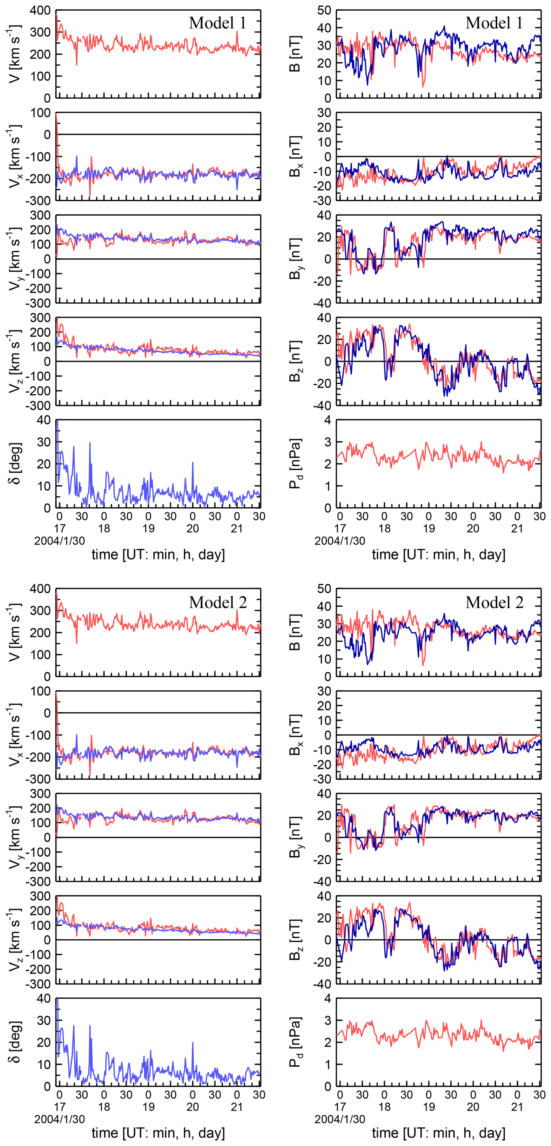
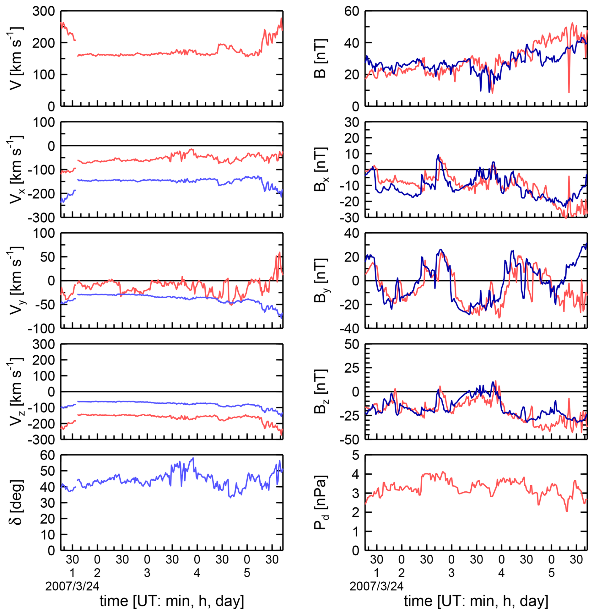
Figure 1 Observed (red lines) and modeled (blue lines) quantities for the passage through the Earth's MSH in case 7. Left panels: from top the velocity magnitude V, GSE velocity components V_x, V_y, and V_z, and the angle δ between the observed and modeled velocity vectors; right panels: from top the magnetic field magnitude B, GSE magnetic field components B_x, B_y, and B_z, and upstream dynamic pressure P_d. Upper panels are for Model 1, bottom panels for Model 2. The left-hand-side panel model velocity components (light blue) are proxy values, created using an artificial radial upstream magnetic field, while the model MSH magnetic field components on the right-hand-side panels (dark blue) use the actual upstream IMF observations.

Table 1 List of the MSH Crossings.

Based on our experience gained in Vandas and Romashets (2024), we use here three MSH models which describe potential (current-free) magnetic fields between two confocal paraboloids (Kobel and Flückiger, 1994), two non-confocal paraboloids (Romashets and Vandas, 2019), and two non-confocal spheroids (Vandas and Romashets, 2019). In the cited work, we expected that the model with non-confocal paraboloids would perform better than that with confocal ones, because the geometry of the Vandas and Romashets (2019) model better reflects the reality, but this was not the case. Their performance (measured as mean deviation between model and observed magnetic field vectors) was very similar.

Spreiter and Rizzi (1974) note that a field-aligned flow in the SW will stay field-aligned everywhere. Applying it for the MSH, it means that flow lines here coincide with magnetic field lines when the upstream IMF is radial. Let us assume that MSH flow do not depend on actual IMF direction and magnitude (this is a hypothesis). In this way, Kobel and Flückiger (1994) suggested that their magnetic field lines in the MSH might serve as flow lines if the upstream magnetic field is set radial in their model. Tátrallyay and Erdős (2002), Tátrallyay et al. (2008), and Génot et al. (2009) used this hypothesis when analyzing waves and plasma instabilities in the MSH. Génot et al. (2011) elaborated a comprehensive model of the plasma flow in the MSH, based on this hypothesis and the Kobel and Flückiger (1994) model. Soucek and Escoubet (2012) tested the mentioned flow model with observations in a statistical way and reported a fairly good agreement. Schmid et al. (2021) applied the flow model to the MSH of Mercury, anticipating a future comparison with observations. With the three magnetic-field models in hand, we test the hypothesis in a way similar to our dealing with magnetic-field observations (Vandas and Romashets, 2024).

We artificially set the IMF upstream direction radial in the models, derive magnetic field lines and take them as model flow lines. Then using the actual upstream IMF in the models, we get model magnetic field lines and field magnitudes. Finally we compare model quantities with observed ones in the MSH, with a special emphasis on flow directions.

2 Modeling of the plasma flow direction in the MSH

This modeling is based on the hypothesis by Kobel and Flückiger (1994) and Soucek and Escoubet (2012), that flow streamlines in the MSH would coincide with magnetic field lines if the upstream magnetic field is radial (regardless of the actual IMF direction and magnitude). We proceed in this way. Shapes of the BS and MP follow from their models, SW dynamic pressure, and real BS and MP crossings, and determine the shape of the MSH for each instance. A model of the MSH magnetic field under the assumption that the upstream magnetic field is radial yields a magnetic field configuration in the MSH, magnetic field lines of which are in fact flow streamlines (according to the hypothesis). The flow streamlines determine flow directions which can be compared with observed directions, thus testing the hypothesis. We do not model velocity magnitude, because it needs additional assumptions going beyond the scope of this paper. The model magnetic field for comparison with observations is determined using the actual upstream IMF (as it was done in Vandas and Romashets, 2024).

In the following subsections we describe BS and MP models and MSH magnetic field models used in the present paper. Only analytical models are included. We consider four BS and MP models, and three MSH magnetic-field models, which are potential (current-free) models, two of them assume axially symmetric paraboloidal BS and MP shapes, and the third one is of spheroidal shapes of the BS and MP. Magnetic fields in the MSH depends on BS and MP shapes (i.e., on a_ij coefficients described below) and on the upstream magnetic field, which is assumed homogeneous. All of these quantities change in time according to varying upstream conditions, that is, the dynamical pressure (specifying the a_ij coefficients) and the upstream magnetic field vector, which are known from observations.

2.1 BS and MP Shapes

Determination of the BS and MP shapes follows the method described in Vandas and Romashets (2024). We work in aberrated coordinate system. Its relationship to the GSE (Geocentric Solar Ecliptic) system is shown in detail in Vandas et al. (2020). Its center is the Earth's center and the x axis is a common rotational symmetry axis for BS and MP models used here. We assume that the BS and MP have spheroidal or paraboloidal shapes (always the same types for both), which are defined by coefficients a₁₁, a₁₄, a₄₄, and equations

$$\begin{array}{}\text{(1)}& {\displaystyle }{a}_{\mathrm{11},\mathrm{BS}}{x}_{\mathrm{BS}}^{\mathrm{2}}+y_{\mathrm{BS}}^{\mathrm{2}}+z_{\mathrm{BS}}^{\mathrm{2}}+a_{\mathrm{14},\mathrm{BS}}{x}_{\mathrm{BS}}+a_{\mathrm{44},\mathrm{BS}}=\mathrm{0},\text{(2)}& {\displaystyle }{a}_{\mathrm{11},\mathrm{MP}}{x}_{\mathrm{MP}}^{\mathrm{2}}+y_{\mathrm{MP}}^{\mathrm{2}}+z_{\mathrm{MP}}^{\mathrm{2}}+a_{\mathrm{14},\mathrm{MP}}{x}_{\mathrm{MP}}+a_{\mathrm{44},\mathrm{MP}}=\mathrm{0}.\end{array}$$

The subscripts BS or MP at coordinates stress that the points are located at the BS or MP. For the time when a satellite crossed the BS, it holds

$$\begin{array}{}\text{(3)}& \begin{array}{rl}{a}_{\mathrm{11},\mathrm{BS}}^{\left(\mathrm{BS}\right)}& {\left[x_{\mathrm{BS}}^{\left(\mathrm{BS}\right)}\right]}^{\mathrm{2}}+{\left[y_{\mathrm{BS}}^{\left(\mathrm{BS}\right)}\right]}^{\mathrm{2}}+{\left[z_{\mathrm{BS}}^{\left(\mathrm{BS}\right)}\right]}^{\mathrm{2}}+a_{\mathrm{14},\mathrm{BS}}^{\left(\mathrm{BS}\right)}{x}_{\mathrm{BS}}^{\left(\mathrm{BS}\right)}\\ & +a_{\mathrm{44},\mathrm{BS}}^{\left(\mathrm{BS}\right)}=\mathrm{0},\end{array}\end{array}$$

where $x_{\mathrm{BS}}^{\left(\mathrm{BS}\right)}$, $y_{\mathrm{BS}}^{\left(\mathrm{BS}\right)}$, and $x_{\mathrm{BS}}^{\left(\mathrm{BS}\right)}$ are coordinates of the BS crossing, the time of the BS crossing is indicated by BS in parentheses. Similarly, for the MP crossing, we have

$$\begin{array}{}\text{(4)}& \begin{array}{rl}{a}_{\mathrm{11},\mathrm{MP}}^{\left(\mathrm{MP}\right)}& {\left[x_{\mathrm{MP}}^{\left(\mathrm{MP}\right)}\right]}^{\mathrm{2}}+{\left[y_{\mathrm{MP}}^{\left(\mathrm{MP}\right)}\right]}^{\mathrm{2}}+{\left[z_{\mathrm{MP}}^{\left(\mathrm{MP}\right)}\right]}^{\mathrm{2}}+a_{\mathrm{14},\mathrm{MP}}^{\left(\mathrm{MP}\right)}{x}_{\mathrm{MP}}^{\left(\mathrm{MP}\right)}\\ & +a_{\mathrm{44},\mathrm{MP}}^{\left(\mathrm{MP}\right)}=\mathrm{0}.\end{array}\end{array}$$

The coordinates of the crossings are known and we need to determine six a-coefficients. Two equations for them have been just listed, the remaining four are specific for BS and MP models used and will be described later. The coefficients for the BS crossing fix the BS shape for the upstream dynamical pressure $P_{\mathrm{d}}^{\left(\mathrm{BS}\right)}$ (following from data) at this time, and similarly for the MP crossing and corresponding upstream dynamical pressure $P_{\mathrm{d}}^{\left(\mathrm{MP}\right)}$. For a general time and corresponding upstream dynamical pressure, P_d, the shapes of the BS and MP are given by Eqs. (1)–(2) with

$$\begin{array}{}\text{(5)}& {\displaystyle }\begin{array}{rl}{a}_{\mathrm{11},\mathrm{BS}}& =a_{\mathrm{11},\mathrm{BS}}^{\left(\mathrm{BS}\right)},a_{\mathrm{14},\mathrm{BS}}=a_{\mathrm{14},\mathrm{BS}}^{\left(\mathrm{BS}\right)}{\left[{\displaystyle \frac{P_{\mathrm{d}}^{\left(\mathrm{BS}\right)}}{P_{\mathrm{d}}}}\right]}^{\frac{\mathrm{1}}{{\mathit{\epsilon }}_{\mathrm{BS}}}},\\ & a_{\mathrm{44},\mathrm{BS}}=a_{\mathrm{44},\mathrm{BS}}^{\left(\mathrm{BS}\right)}{\left[{\displaystyle \frac{P_{\mathrm{d}}^{\left(\mathrm{BS}\right)}}{P_{\mathrm{d}}}}\right]}^{\frac{\mathrm{2}}{{\mathit{\epsilon }}_{\mathrm{BS}}}},\end{array}\text{(6)}& {\displaystyle }\begin{array}{rl}{a}_{\mathrm{11},\mathrm{MP}}& =a_{\mathrm{11},\mathrm{MP}}^{\left(\mathrm{MP}\right)},a_{\mathrm{14},\mathrm{MP}}=a_{\mathrm{14},\mathrm{MP}}^{\left(\mathrm{MP}\right)}{\left[{\displaystyle \frac{P_{\mathrm{d}}^{\left(\mathrm{MP}\right)}}{P_{\mathrm{d}}}}\right]}^{\frac{\mathrm{1}}{{\mathit{\epsilon }}_{\mathrm{MP}}}},\\ & a_{\mathrm{44},\mathrm{MP}}=a_{\mathrm{44},\mathrm{MP}}^{\left(\mathrm{MP}\right)}{\left[{\displaystyle \frac{P_{\mathrm{d}}^{\left(\mathrm{MP}\right)}}{P_{\mathrm{d}}}}\right]}^{\frac{\mathrm{2}}{{\mathit{\epsilon }}_{\mathrm{MP}}}}.\end{array}\end{array}$$

The last relationships follow from a common assumption in which the BS and MP radially shrink or expand in a dependence on P_d, more specifically coordinates of BS and MP points behave as $x_{\mathrm{BS}}\propto P_{\mathrm{d}}^{-\frac{\mathrm{1}}{{\mathit{\epsilon }}_{\mathrm{BS}}}}$, and so on for the other coordinates (note that there are misprints in Eqs. (3) and (6) in Vandas and Romashets (2024), there are missing minus signs in all exponents). The constants ε_BS and ε_MP are specified by the BS and MP models. The dynamical pressure is calculated by the formula $P_{\mathrm{d}}=\mathrm{1.2}{n}_{\mathrm{p}}{m}_{\mathrm{p}}{V}_{\mathrm{sw}}^{\mathrm{2}}$, where n_p is the upstream proton number density, m_p is the proton mass, V_sw is the upstream SW velocity, and the factor 1.2 accounts for the presence of alpha particles (helium) in the SW.

2.2 Magnetic Field Model 1

Model 1 is the Kobel and Flückiger (1994) model, which have paraboloidal BS and MP with the same foci, which are situated halfway between the MP nose and the Earth's center (the origin of coordinates). This means that

$$\begin{array}{}\text{(7)}& a_{\mathrm{11},\mathrm{BS}}=\mathrm{0},a_{\mathrm{11},\mathrm{MP}}=\mathrm{0},\end{array}$$

and the common foci and their placement yield additional two equations

$$\begin{array}{}\text{(8)}& {\displaystyle \frac{a_{\mathrm{44},\mathrm{BS}}}{a_{\mathrm{14},\mathrm{BS}}}}+{\displaystyle \frac{a_{\mathrm{14},\mathrm{BS}}}{\mathrm{4}}}={\displaystyle \frac{a_{\mathrm{44},\mathrm{MP}}}{\mathrm{2}{a}_{\mathrm{14},\mathrm{MP}}}},\text{(9)}& {\displaystyle \frac{a_{\mathrm{44},\mathrm{MP}}}{a_{\mathrm{14},\mathrm{MP}}}}+{\displaystyle \frac{a_{\mathrm{14},\mathrm{MP}}}{\mathrm{4}}}={\displaystyle \frac{a_{\mathrm{44},\mathrm{MP}}}{\mathrm{2}{a}_{\mathrm{14},\mathrm{MP}}}}.\end{array}$$

The magnetic field components are given in Kobel and Flückiger (1994). We set ${\mathit{\epsilon }}_{\mathrm{BS}}={\mathit{\epsilon }}_{\mathrm{MP}}=\mathrm{6}$, as commonly used values for them.

2.3 Magnetic Field Model 2

Model 2 is the Romashets and Vandas (2019) model, which also have paraboloidal BS and MP but their foci need not coincide. The BS and MP positions and shapes are determined by the Jelínek et al. (2012) model, so we have

$$\begin{array}{}\text{(10)}& {\displaystyle }{a}_{\mathrm{11},\mathrm{BS}}=\mathrm{0},a_{\mathrm{11},\mathrm{MP}}=\mathrm{0},\text{(11)}& {\displaystyle \frac{a_{\mathrm{44},\mathrm{BS}}}{a_{\mathrm{14},\mathrm{BS}}^{\mathrm{2}}}}=-{\displaystyle \frac{{\mathit{\lambda }}_{\mathrm{BS}}^{\mathrm{2}}}{\mathrm{4}}},{\displaystyle \frac{a_{\mathrm{44},\mathrm{MP}}}{a_{\mathrm{14},\mathrm{MP}}^{\mathrm{2}}}}=-{\displaystyle \frac{{\mathit{\lambda }}_{\mathrm{MP}}^{\mathrm{2}}}{\mathrm{4}}},\end{array}$$

with λ_BS=1.17 and λ_MP=1.54. Moreover, ε_BS=6.55 and ε_MP=5.26. These four values are given in the Jelínek et al. (2012) model. The magnetic field components follow from Romashets and Vandas (2019).

2.4 Magnetic Field Model 3

Model 3 is the Vandas and Romashets (2019) model, which has spheroidal BS and MP, and their foci may not coincide. The BS and MP positions and shapes are determined by simplified Formisano (1979) and Formisano et al. (1979) models, namely that the a_ij coefficients save the proportions as in Formisano's BS and MP models,

$$\begin{array}{}\text{(12)}& \begin{array}{rl}& a_{\mathrm{11},\mathrm{BS}}=a_{\mathrm{11}\mathrm{na},\mathrm{BS}},{\displaystyle \frac{a_{\mathrm{14},\mathrm{BS}}^{\mathrm{2}}}{a_{\mathrm{44},\mathrm{BS}}}}={\displaystyle \frac{a_{\mathrm{14}\mathrm{na},\mathrm{BS}}^{\mathrm{2}}}{a_{\mathrm{44}\mathrm{na},\mathrm{BS}}}},\\ & a_{\mathrm{11},\mathrm{MP}}=a_{\mathrm{11}\mathrm{na},\mathrm{MP}},{\displaystyle \frac{a_{\mathrm{14},\mathrm{MP}}^{\mathrm{2}}}{a_{\mathrm{44},\mathrm{MP}}}}={\displaystyle \frac{a_{\mathrm{14}\mathrm{na},\mathrm{MP}}^{\mathrm{2}}}{a_{\mathrm{44}\mathrm{na},\mathrm{MP}}}},\end{array}\end{array}$$

where coefficients with the subscript na are the scaled Formisano's coefficients in the aberrated system: $a_{\mathrm{11}\mathrm{na},\mathrm{BS}}=\mathrm{0.52}$, $a_{\mathrm{14}\mathrm{na},\mathrm{BS}}=\mathrm{47.53}$, $a_{\mathrm{44}\mathrm{na},\mathrm{BS}}=-\mathrm{613}$, $a_{\mathrm{11}\mathrm{na},\mathrm{MP}}=\mathrm{0.65}$, $a_{\mathrm{14}\mathrm{na},\mathrm{MP}}=\mathrm{21.41}$, and $a_{\mathrm{44}\mathrm{na},\mathrm{MP}}=-\mathrm{221}$ (see Vandas et al., 2020). It is set ${\mathit{\epsilon }}_{\mathrm{BS}}={\mathit{\epsilon }}_{\mathrm{MP}}=\mathrm{6}$. The magnetic field components are given in Vandas and Romashets (2019).

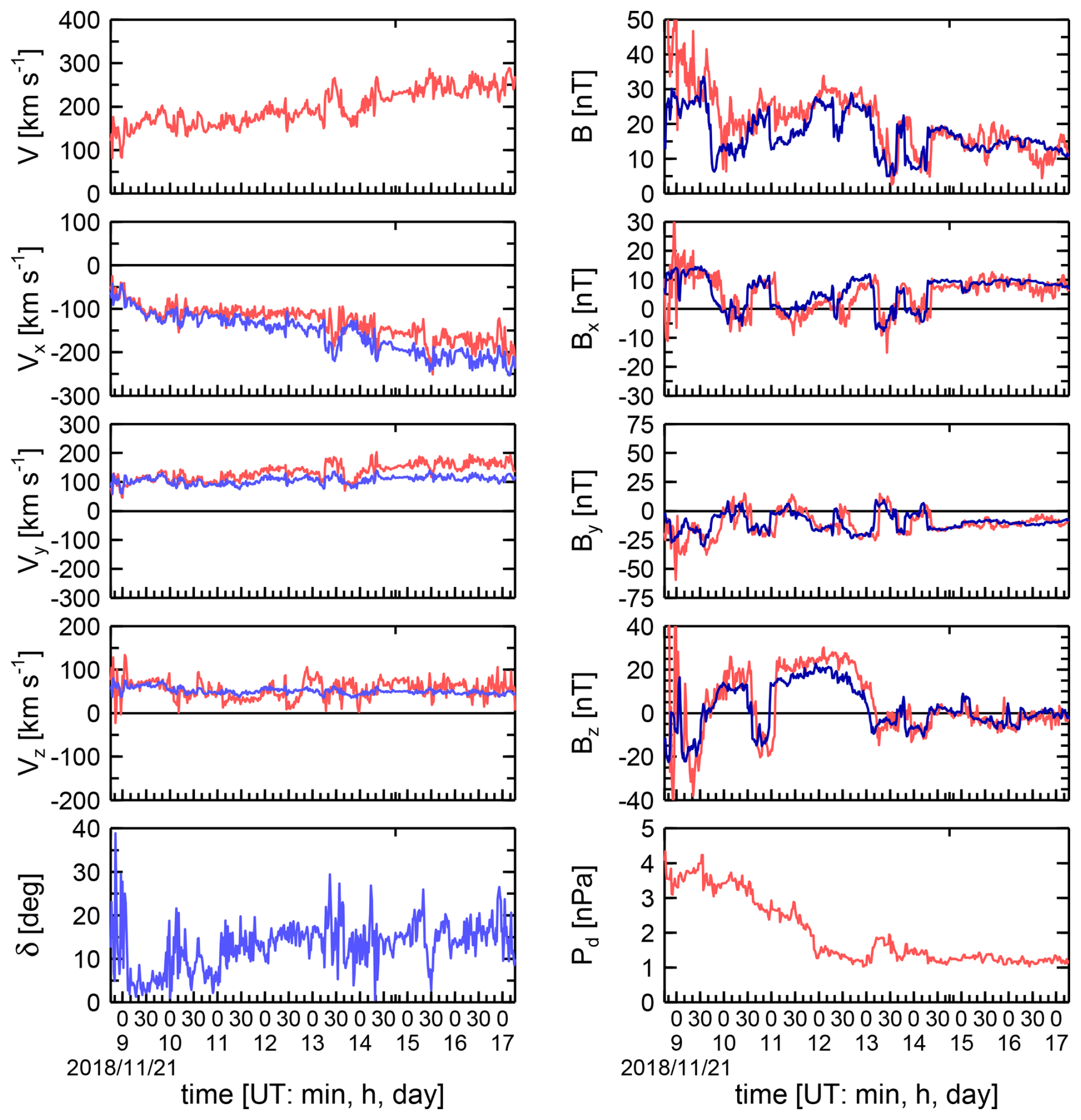
Figure 2 Observed and modeled quantities in the MSH for case 43. Only results of Model 1 are shown, otherwise the format is the same as for Fig. 1.

Table 2 Performance of the Models According to δ_avg.

3 Data

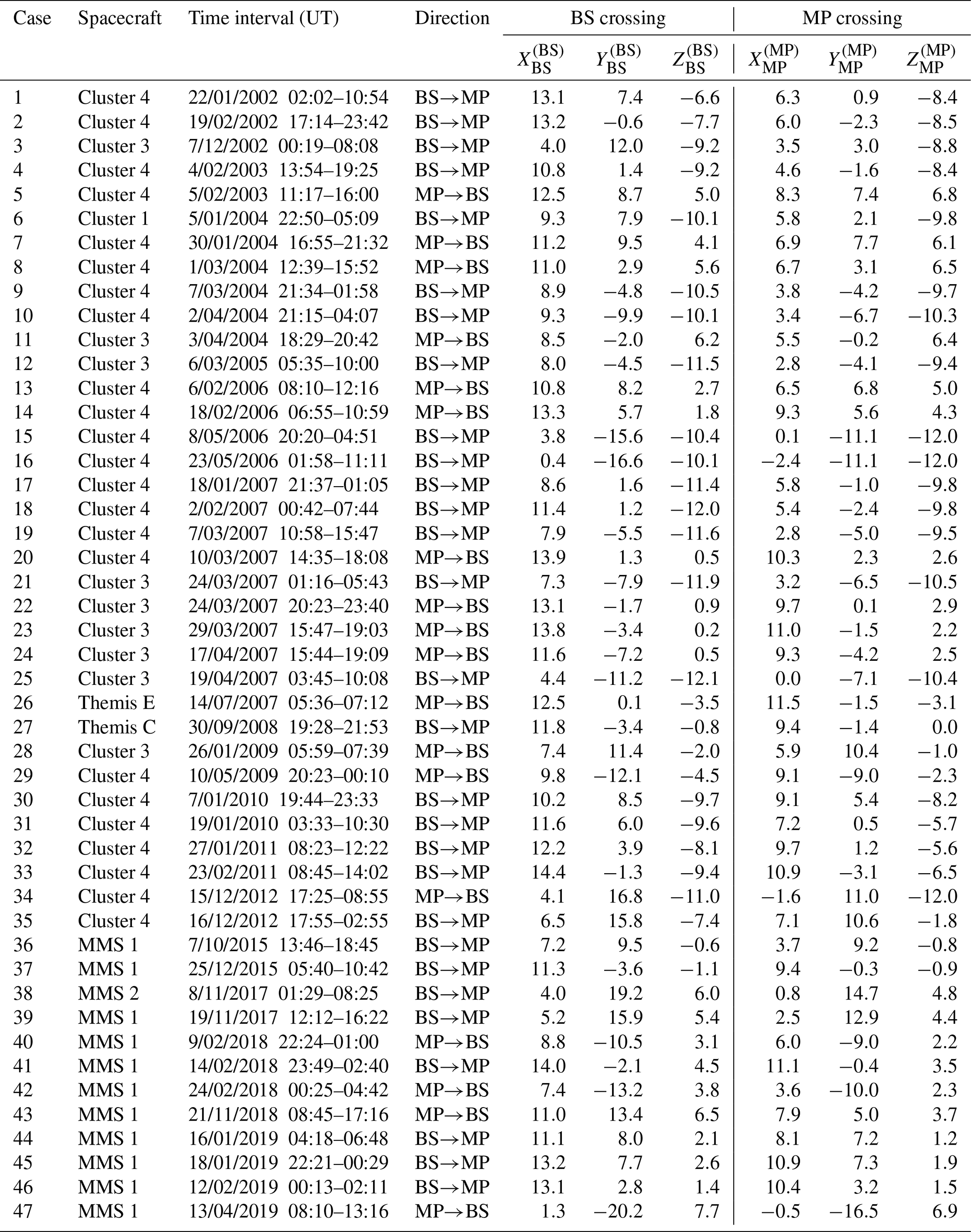
We used observations during MSH passages by Cluster, Themis, and MMS spacecraft. There are many such passages but our quite stringent criteria limited cases very much. We required a passage to be at least a few hours long, contained both plasma and magnetic field measurements, BS and MP crossings to be clearly identifiable, and upstream data for moments of BS and MP crossings are known. The passages were bordered by a BS crossing at one side and an MP crossing at the other side, cases with multiple crossings were excluded. Times of crossings were determined by visual inspection of observed time profiles according to characteristic jumps of magnetic field and plasma quantities (e.g., expected changes in velocity and magnetic field components, density, and temperature at the BS and MP). OMNI data for determination of upstream conditions were utilized. We got 47 cases which are listed in Table 1. Columns from left to the right show the case number, spacecraft, time interval of the passage (when the second time is lower than the first time, it means the next day), direction of the passage, and coordinates (in GSE system; units are R_E, where R_E is the Earth's radius) of the satellites at moments of the BS and MP crossings. Note that the coordinates are in capital letters in order to distinguish them from the lower-case coordinates (used, e.g., in Eq. 3), which are coordinates in the aberrated system. Nevertheless, the latter ones are calculated from the former ones using the relationships given in Vandas et al. (2020). Data for the MSH passages were taken from the World Data Center (WDC) at NASA GSFC (http://cdaweb.gsfc.nasa.gov/cdaweb/, last access: 4 September 2024). We used 1 min averages provided by WDC from Cluster (magnetic field: FGM instrument, PIs A. Balogh & E. Lucek, data source CP_FGM_SPIN; plasma velocity: CIS instrument, PI H. Rème, data source PP_CIS), Themis (magnetic field: FGM instrument, PIs V. Angelopoulos, U. Auster, K. H. Glassmeier, & W. Baumjohann, data source l2_fgm; plasma velocity: ESA instrument, PIs V. Angelopoulos, C. W. Carlson & J. McFadden, data source l2_mom), and MMS (magnetic field: FGM instrument, PIs J. Burch, C. Russell, & W. Magnus, data source fgm_srvy_l2; plasma velocity: DIS instrument, PIs J. Burch, C. Pollock, & B. Giles, data source fpi_fast_l2_dis-moms). For determination of upstream magnetic field and dynamical pressure, 1-min averages of OMNI Plus data (Wind KP shifted to the BS nose; when not available, ACE_bsn) from WDC (https://omniweb.gsfc.nasa.gov/, last access: 4 September 2024) were used.

Figure 3 Observed and modeled quantities in the MSH for case 21. The format is the same as in Fig. 2.

4 Results

We calculated MSH model magnetic field configurations for the MSH passages listed in Table 1 two times, for the upstream magnetic field vector from OMNI, and for the upstream radial field (i.e., only the x component present). Each observation in the MSH (with 1 min cadence) was supplemented by these model magnetic field vectors (calculated at real spacecraft positions and provided that the necessary upstream values were known), and resulting observed and model profiles were compared. It means that for each time, magnetic field configurations were calculated anew, because the upstream plasma dynamic pressure and magnetic field vector generally changed, and so did the positions and shapes of the BS and MP. The modeled magnetic field vectors were uniquely determined by the upstream values and a MSH model used, there were no free parameters or tailoring. An artificial upstream radial IMF was used as an input to model the MSH magnetic field, which then served as a proxy for the modeled MSH velocity vector.

An example of the profile comparisons is shown in Fig. 1. It is case 7 from Table 1. There are four groups of panels (2×2), left panels deal with velocity profiles, right panels with magnetic-field profiles in the MSH. Because the velocity magnitude was not modeled, we took it from the observed values for calculations of the modeled velocity vectors, but their directions followed from the modeled values. The δ is the angle between the observed and modeled velocity vectors,

$$\begin{array}{}\text{(13)}& \mathit{\delta }=\arccos {\displaystyle \frac{{\mathbf{V}}^{\left(\mathrm{obs}\right)}\cdot {\mathbf{B}}^{\left(\mathrm{rmod}\right)}}{\left|{\mathbf{V}}^{\left(\mathrm{obs}\right)}\right|\left|{\mathbf{B}}^{\left(\mathrm{rmod}\right)}\right|}}\end{array}$$

where B^(rmod) is a modeled magnetic field in the MSH when the upstream magnetic field is set radial. A low value of δ indicates a good match in the flow direction. Top groups of panels in Fig. 1 show results for Model 1, bottom groups for Model 2 for comparison. We see that the modeled profiles follow relatively well the observed ones in this case for both the magnetic field and velocity. Larger discrepancies are mainly near the MP, a feature already noticed in our previous papers. In addition, we can see that there are no significant differences in the results between Models 1 and 2. Therefore in the following figures with profiles we display only that for Model 1. One can observe that quite large variations in the magnetic field components are relatively well matched by the model.

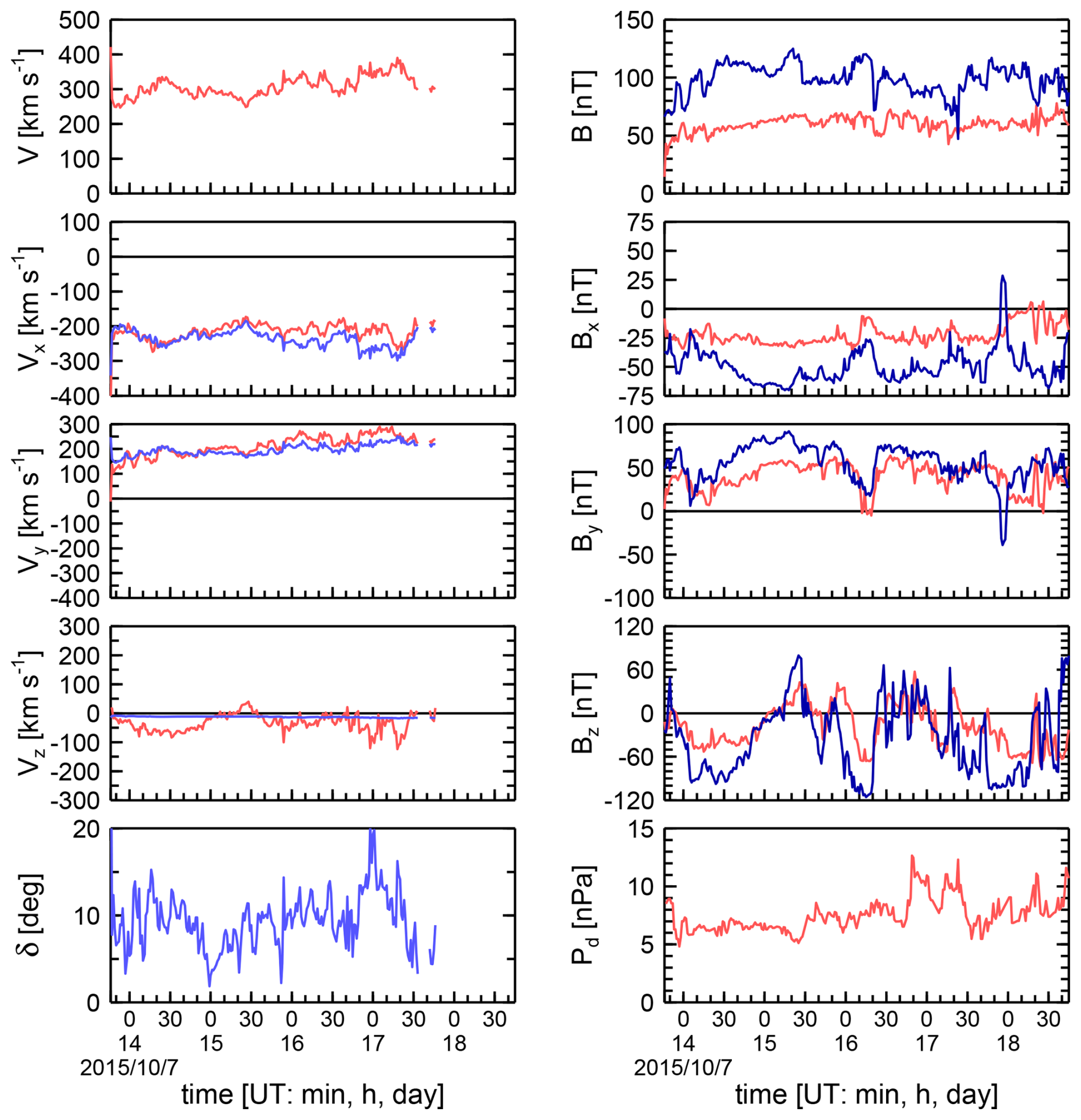
Figure 4 Observed and modeled quantities in the MSH for case 36. The format is the same as in Fig. 2.

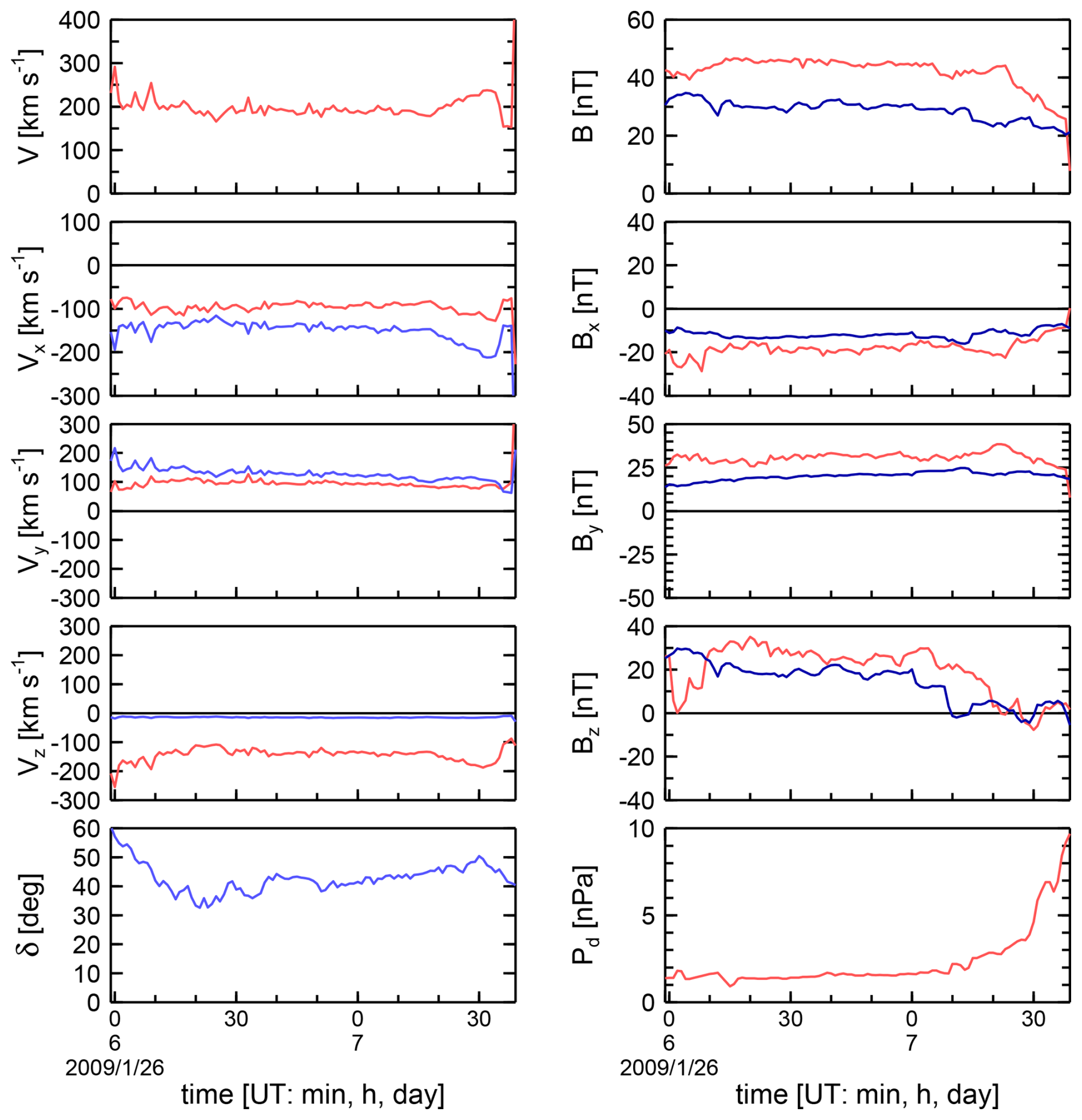
Figure 5 Observed and modeled quantities in the MSH for case 28. The format is the same as in Fig. 2.

Figure 2 displays case 43 when a large change in the dynamical pressure occurred. The observed profiles are quite well matched by modeled ones. If magnetic field profiles are satisfactorily met by a model, it does not guarantee that velocity directions will be met, as Fig. 3 demonstrates, and vice versa (Fig. 4). Figure 5 is an example when models fail for both magnetic field and velocity directions.

The quality of the plasma-flow-direction match was measured by averaged δ's (Eq. 13) for each case,

$$\begin{array}{}\text{(14)}& {\mathit{\delta }}_{\mathrm{avg}}={\displaystyle \frac{\mathrm{1}}{N}}\sum _{i=\mathrm{1}}^N{\mathit{\delta }}_i={\displaystyle \frac{\mathrm{1}}{N}}\sum _{i=\mathrm{1}}^N\arccos {\displaystyle \frac{{\mathbf{V}}_i^{\left(\mathrm{obs}\right)}\cdot {\mathbf{B}}_i^{\left(\mathrm{rmod}\right)}}{\left|{\mathbf{V}}_i^{\left(\mathrm{obs}\right)}\right|\left|{\mathbf{B}}_i^{\left(\mathrm{rmod}\right)}\right|}}\end{array}$$

where N is a number of compared values for a given passage. We used this measure to summarize results over all our cases. For each case, we ranked the three models according to values δ_avg as 1 (the best, i.e., it has a lowest value), 2, or 3.

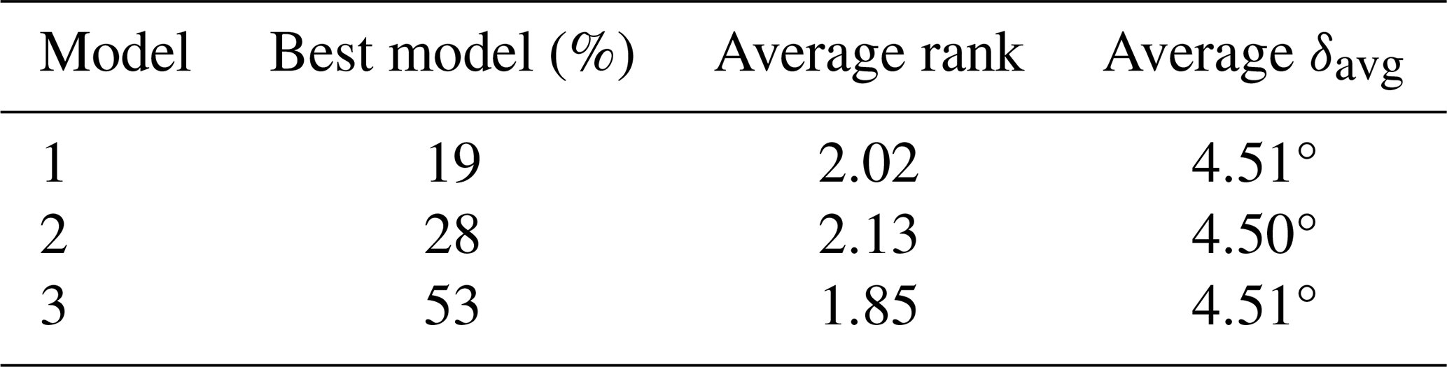
Table 2 lists percentages when the models were the best (the second column) and averaged ranks over cases (the third column). We see that differences among models are marginal. The δ_avg averaged over cases is practically the same for all models, and it is satisfactorily low (below 5°), indicating on average an acceptable agreement between magnetic field lines of a particular magnetic field configuration and flow lines.

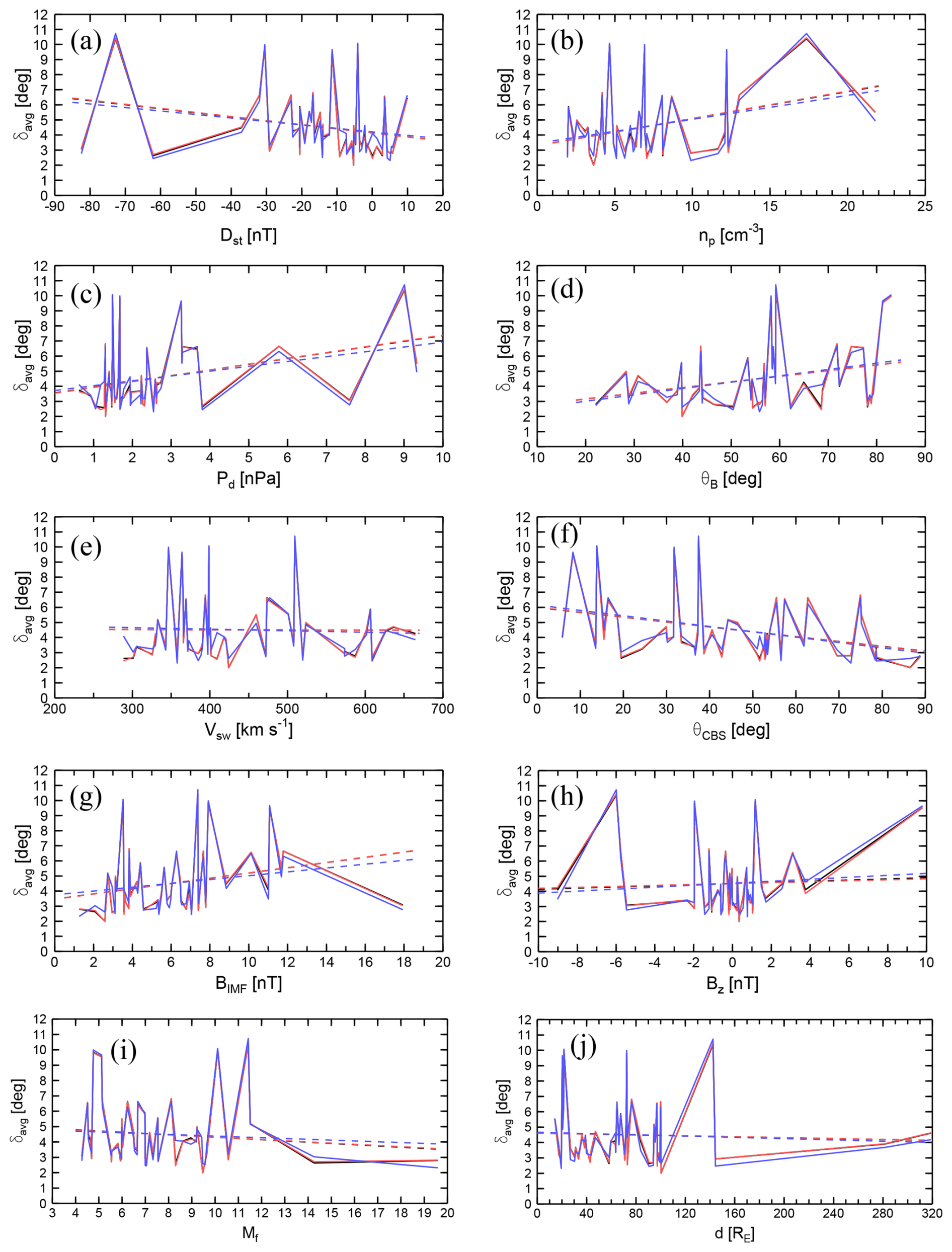
Figure 6 Dependencies of δ_avg on various quantities. The details are given in the text. Model 1 is drawn in the black lines (which are mostly obscured by the red ones), Model 2 in the red lines, and Model 3 in the blue lines.

Figure 6a shows a dependency of our quality measure δ_avg on D_st. A D_st value for a particular case means its average over the related MSH passage. And it is also done in such a way for the other quantities shown in the other panels. One can see that there are no significant differences in behavior of the models, but there are large fluctuations in values and no neat dependency. We can only judge on trends making linear regression in a form of dashed lines with the same color coding as for the solid lines. The models of the MSH plasma flow perform slightly worse with increasing geomagnetic activity. A similar situation is with the dynamical pressure P_d (Fig. 6c). Agreement with the model plasma flow directions becomes worse with a P_d increase. Analogically this holds for the upstream magnetic field magnitude B_IMF (Fig. 6g). There is no trend for the upstream SW velocity V_sw (Fig. 6e), so there must be an increase in δ_avg with increasing upstream density n_p, as Fig. 6b confirms. There also are no trends for the upstream B_z (Fig. 6h), and fast magnetosonic Mach number M_f (Fig. 6i). The trend for the upstream magnetic-field cone angle θ_B (Fig. 6d) indicates that the plasma flow directions are better modeled when the upstream magnetic field is close to radial. It can indicate that the hypothesis mentioned in Introduction and on which modeling of flow directions relies, may weaken for large θ_B. Figure 6f shows that the average deviations between observed and modeled velocities are larger for small cone angles θ_CBS (Sun-Earth-spacecraft angles), i. e. positions near the subsolar bow shock. In the subsolar region of the MSH, changes in the direction of the plasma flow towards the MP are relatively the largest, so potential deviations from model values are more pronounced.

5 Discussion

The presented comparison relies on simplifying assumptions which surely affect observed profiles. The real BS and MP are not axisymmetric and their shapes significantly differ from the model shapes farther from the subsolar region.

Magnetic reconnection causes erosion and thus MP and BS movements inward during periods of southward IMF orientation. This effect is not included in our simple modeling. However, there is no trend in δ_avg versus B_z seen in Fig. 6h. An explanation might be that we use actual positions of the MP and BS at times of crossings, i.e., already after a possible erosion.

Largest discrepancies between model values and observations are near the MP. We have already noticed this fact when dealing with a comparison of magnetic field components (Vandas et al., 2020). As in the cited paper, we explain it by presence of boundary layers and the magnetic barrier near the MP, which are not taken into account in the simple models used here.

We assume that upstream IMF and SW plasma values do not spatially vary along the BS (which is a simplification of a real situation), and these values are taken from spacecraft observations (by Wind or ACE as SW monitors), situated at relatively large distances from the Earth, so time-shifted to the BS nose for time-synchronization with the MSH observations. Figure 6j shows δ_avg versus the distance d of the SW monitor from the Sun-Earth line. No clear trend in the values of delta with distance d is observed. This is also supported by our supplementary examination. We calculated the averaged delta for several cases from Table 1 two times, using alternatively Wind and ACE as the upstream input. Resultant deltas for Wind and ACE do not differ more than about 1°, even though the positions of Wind and ACE were very different.

We see large variations of δ_avg in Fig. 6 which occur throughout all plots. We tried to find a cause. Therefore we plotted dependencies of δ_avg on various parameters (Fig. 6 shows some) in an effort that δ_avg will be better ordered for some parameters, but in vain. Then we focused on several cases with large deltas but did not find any clear reason for them when comparing these cases with the other ones.

The dashed lines in Fig. 6 are not considered as fits which should predict δ_avg for given values. Rather they are used to show trends, i.e. a general increase or decrease. We mean by no trend a difference in δ_avg (as given by the dashed lines) lower than about 1°.

6 Conclusions

We examined plasma flow directions in the MSH and compared them with modeled quantities. Three current-free MSH models were used and the hypothesis that flow lines coincide with magnetic field lines when the upstream magnetic field is set radial. The quality of the match was measured by the averaged angle δ_avg between the observed and modeled plasma flow directions. We found that there are no significant differences in the performances of the models. The models yielded directions of the plasma flow quite satisfactorily on average, the difference averaged over all cases was about 4.5° only. Contrary to the magnetic field modeling, in the case of plasma-flow modeling, the performances mildly depend on values of the dynamic pressure or geomagnetic activity (worse with higher values). The models better describe the plasma flow directions for passages farther from the subsolar point, or when the upstream magnetic field is closer to radial.

Because the performances of the models are comparable, we recommend to use the Kobel and Flückiger (1994) model, which is simpler and much faster in yielding results than the other models.