Properties of large-amplitude kilometer-scale field-aligned currents at auroral latitudes, as derived from Swarm satellites

High-resolution magnetic field recordings by the Swarm A and C spacecraft have been used to investigate the properties of field-aligned currents (FACs) at auroral latitudes down to their smallest scales (<1 km). Particularly suitable for that purpose are the magnetic field recordings, taken at a rate of 50 Hz, during the 2 weeks around the quasi-coplanar orbit configuration around 1 October 2021. We have split the recorded signal caused by FACs of along-track scales from 0.2 to 20 km into 8 quasi-logarithmically spaced ranges. Our investigations revealed that the kilometer-scale FACs (0.2–5 km) show quite different characteristics from those of the small-scale FACs (5–20 km). The kilometer-scale FACs exhibit short-lived (<1 s) randomly appearing large current spikes. They are confined to certain latitude ranges, which depend on local time. Small-scale FAC structures last for longer times (>10 s) and are distributed over larger latitude ranges. Their largest amplitudes are achieved at latitudes that overlap with the kilometer-scale FACs. The small-scale FACs have earlier been identified as Alfvén waves that are partly reflected at the ionosphere, and they can oscillate within the ionospheric Alfvén resonator. When at the same time additional Alfvén waves are launched from the magnetosphere they will interfere with the reflected. We suggest that the interaction between oppositely travelling Alfvén waves, when continuing sufficiently long, is generating the large-amplitude and short-lived kilometer-scale FACs.

1 Introduction

Field-aligned currents (FAC) in the ionosphere are a commonly observed phenomenon. In particular, at auroral latitudes they act as coupling agents between plasma processes in the magnetosphere and the ionosphere. FACs exhibit horizontal scales in the ionosphere from less than 1 km (e.g., Neubert and Christiansen, 2003; Rother et al., 2007) up to some 1000 km (e.g., Iijima and Potemra, 1976; Anderson et al., 2014). In general, the current densities become larger the smaller the scale of the FAC. In most cases, pairs of upward and downward currents appear close together. Thus, small-scale FACs, with their high density, contribute only little to the net current between magnetosphere and ionosphere, but they can transfer a significant amount of energy into the ionospheres (e.g., Lühr et al., 2004).

Multi-spacecraft missions have been used to evaluate the properties of FACs with different sizes. For example, Gjerloev et al. (2011) made use of the three ST5 satellites in pearls-on-a-string formation. By comparing the magnetic field readings of successive spacecraft, they found that FACs with scales larger than 100 km on the nightside can be considered as stationary (for at least 1 min), while on the dayside this was only valid at scales above 200 km. With the help of the three Swarm satellites Lühr et al. (2015) confirmed these findings and extended the analysis to smaller scales down to some 10 km. Those FACs exhibited a lot of temporal variability at periods of about 10 s and could not be treated as stationary structures. At those scales magnetic field lines cannot be regarded any longer as equipotential lines.

In a recent study, Lühr and Zhou (2025) extended the FAC scale analysis at auroral latitudes by making use of the Swarm Counter-Rotating Orbit Phase in 2021. During that campaign the orbits of Swarm A and C were brought close together, and Swarm B cycled the Earth in opposite direction. Around 1 October 2021 all three orbital planes were quasi-coplanar. Thereafter, the orbits slowly separated again. By means of a cross-correlation analysis it was checked how well the signals at the two spacecraft agree. Over the course of the study period the cross-track separation covered the range between 0 and 30 km at the equator-crossing point, and the along-track separation varied from 2 to 41 s. The campaign results largely confirmed earlier findings. Current structures with apparent periods of more than 15 s (corresponding to along-track wavelengths of >100 km) exhibit good correlations between the magnetic field signals at the two accompanying spacecraft for all experienced along- and cross-track separations. However, for apparent periods of less than 10 s (<75 km wavelength) the properties changed. Here significant correlations were only achieved when the cross-track separation was below about 6 km and the along-track separation below 18 s. These results indicate that FACs at these scales are no longer organized as current sheets but represent current filaments.

Concerning the naming convention for different FAC scale sizes, most studies make use of 1 Hz satellite magnetic field samples. For them about 10 km is the lower limit. Therefore, the term small-scale FACs is found frequently in the literature for sizes 10–50 km (e.g. Pakhotin et al., 2018). We will also use this name here for that scale range. For the even smaller current structures (0.5–5 km) we follow the suggestion of Rother et al. (2007) and term them kilometer-scale FACs.

Not much is known about the characteristics of km-scale FACs. Neubert and Christiansen (2003) and Rother et al. (2007) have shown that these narrow FACs can attain very large amplitudes. They appear preferentially on the dayside at high auroral latitudes in the cusp region, around noon and in the prenoon sector. On the nightside, km-scale FACs are generally observed with smaller amplitudes and their appearance coincides with the westward electrojet. No information is available about their temporal and spatial correlation lengths.

This study provides such information by making use of the high-resolution 50 Hz magnetic field samples from the Swarm A and Swarm C satellites. These data provide sufficient resolution for investigating the details of the smallest FAC features. In preparation for the CHAMP satellite mission (Reigber et al., 2002) we made use of the Freja satellite burst mode magnetic field readings, taken at 128 samples per second, to find out the appropriate sample rate for resolving the large-amplitude FACs at smallest scales. As a result of that the 50 Hz sampling was chosen, which captured more than 90 % of the spiky current features. Particularly suitable for our study are the weeks around 1 October 2021, when Swarm A and C orbits were quasi coplanar and the along-track separation reduced to 2 s. This unique dataset will be used for determining the temporal and spatial correlation lengths of these smallest scale FAC features.

In the sections to follow we will first introduce the instruments and data considered here. In Sect. 3 some examples are presented showing typical features of the narrow FACs. For a better characterization of the FACs with various scales Sect. 4 presents a separation of the magnetic field signal into 8 period bands. Section 5 provides a statistical analysis of the FAC signals at different scales by means of their ellipticity properties. A discussion of the results and their relations to earlier publications is presented in Sect. 6. Finally, in Sect. 7 the important findings are summarized and conclusions are drawn.

2 Data and processing approach

ESA's Earth observation mission Swarm was launched on 22 November 2013. It consists of three identical satellites in near-polar orbits at different altitudes. During the first mission phase, starting on 17 April 2014, Swarm A and C were flying almost side-by-side, separated by 1.4° in longitude, at an altitude of about 460 km and an inclination of 87.3°. Swarm B is orbiting the Earth about 60 km higher with an inclination of 88°. This difference in inclination causes a slowly increasing difference in longitude between the two orbital planes amounting to about 2° per month.

After almost 8 years in orbit a counter-rotating configuration was achieved between the Swarm A/C pair and Swarm B (for more details see Xiong and Lühr, 2023). Around 1 October 2021 the orbital planes of Swarm A/C and Swarm B crossed the equator at similar longitudes. During the 2 years before that date the longitudinal separation between Swarm A and C had been slowly decreased, such that orbital coplanarity of Swarm A/C was also achieved on 1 October 2021. Furthermore, the along-track separation between Swarm A and C was varied during the months around coplanarity (see Zhou et al., 2024, Fig. 1). Here we focus on the weeks when the along-track separation was reduced to 2 s.

Each of the three satellites is equipped with a set of six instruments (Friis-Christensen et al., 2008). In this study, we use the data from the Swarm Vector Field Magnetometer (VFM). This fluxgate magnetometer is sampling the field vector at a rate of 50 Hz. For maintaining high data precision over the years, the VFM data are calibrated routinely against the readings of the Absolute Scalar Magnetometer (ASM).

Basis for this study are the Swarm Level-1b 50 Hz magnetic field data with the product identifier “MAGx_HR”, where the lower-case “x” in the product names is a placeholder for the spacecraft names, A, B, or C. The magnetic vector data are given in the North-East-Center (NEC) frame. Of interest here are the magnetic signatures caused by FACs at auroral latitudes. For isolating these signatures from other magnetic field contributions, the geomagnetic field model CHAOS-7.18 (Finlay et al., 2020) is subtracted from the full-field readings. This model represents the contributions of Earth core and crustal fields and the effects of large-scale magnetospheric current systems. Since we are interested in the smallest scales of FAC structures, the data are in addition high-pass filtered with a cutoff frequency of about 0.2 Hz. This removes small biases of the CHAOS model and suppresses the longer-period contributions from E-region current systems like the auroral electrojets or the polar cap return currents.

The bandlimited residuals of the horizontal components, B_x and B_y, are used for studying the magnetic signatures caused by the FACs. From these two components we calculate the deflections of, B_trans, transverse to the flight direction and B_along, aligned with the flight direction. They are derived by the transformation

$$\begin{array}{}\text{(1)}& {\displaystyle }\begin{array}{r}{B}_{\text{trans}}=B_y\cos \left(\mathit{\gamma }\right)-B_x\sin \left(\mathit{\gamma }\right)\\ B_{\text{along}}=B_x\cos \left(\mathit{\gamma }\right)+B_y\sin \left(\mathit{\gamma }\right)\end{array}\end{array}$$

where $\sin \left(\mathit{\gamma }\right)=\cos \left(\text{incl}\right)/\cos \left(\text{lat}\right)$ with incl as orbital inclination and lat as latitude of the measurement point. For application in Eq. (1) γ=γ has to be used on the ascending part of the orbit and $\mathit{\gamma }=\mathit{\pi }-\mathit{\gamma }$ on the descending part. These horizontal components, B_trans and B_along, are sufficient for studying the FAC properties since the field lines are almost vertical at auroral latitudes.

3 Representative examples

In an earlier study, Lühr and Zhou (2025) already made use of the close spacing between the Swarm A and C satellites during the counter-rotating orbit phase. By means of a cross-correlation analysis the correlation length both in space and time could be determined for small- and meso-scale FAC structures. These authors found, as expected, a progressively decreasing persistence in space and time towards smaller current structures. Since we are focusing here on the very small FACs, we tried the same cross-correlation approach with data when the spacecraft were closest together. This occurred during the 16 d, 18 September–4 October 2021.

Figure 1 presents two example orbits from northern hemisphere auroral region crossings on 21 September 2021. Shown are in the top panel of the frames a direct comparison between the magnetic recordings by Swarm A and C. Here the B_trans component is used. This component, perpendicular to the orbit track, shows clearest the variations caused by the FACs. Up to 60° in latitude it is oriented in the east-west direction. Towards higher latitudes B_trans gradually rotates and is aligned with north-south at 87.3° GLat, before turning back to east-west on the downleg track. Furthermore, the time derivative, ΔB_trans, is displayed here since it is directly proportional to the FAC density estimates, as outlined by Lühr and Zhou (2025). A ΔB_trans=10 nT s⁻¹ corresponds to 1.1 µA m⁻² when assuming a perpendicular crossing of a plane FAC sheet. These assumptions are commonly not fulfilled for small-scale FACs and lead to some underestimation of current density. The second panel shows the RMS values of ΔB_trans derived over a 16 s period. Here the red line represents the amplitude of the broad-band signal (0.04–5 s periods), while the black line reflects the amplitude variations of the much weaker long-period variations (2.5–5 s periods). In order to make the amplitudes of the two period ranges more comparable, the RMS values of the 2.5–5 s period curve are multiplied by a factor of 5. The third panel shows the derived lag time, T-lag, for an optimal cross-correlation coefficient. Interestingly, the obtained T-lag values stay, over large parts of the orbital arc, close to the actual along-track spacecraft separations, Δt=2.1 s (listed in the header of the frames). In the bottom panel the peak cross-correlation coefficient, Cc is plotted. Here again, the red dots show the results from the full signal spectrum and the black dots those from the long-period signal. For the broad-band generally quite low correlation coefficients are obtained, well below our threshold of 0.75. Only at subauroral latitudes we find some exceptions. Quite differently, for the long-period signal much larger correlation coefficients (black dots) are derived. Over most parts of the orbit they are above the threshold, Cc>0.75. Obvious departures from that appear at regions of large FAC bursts. There the Cc for the long-period signal drops considerably but does not vanish. Across the bottom of the frames, we have listed information along the orbit of Swarm A. Besides the time there are magnetic latitude (MLat), magnetic local time (MLT), and the cross-track distance, d_cross in km, between Swarm A and C. All the described features of the broad-band and long-period signals can also be found in the lower frame of Fig. 1.

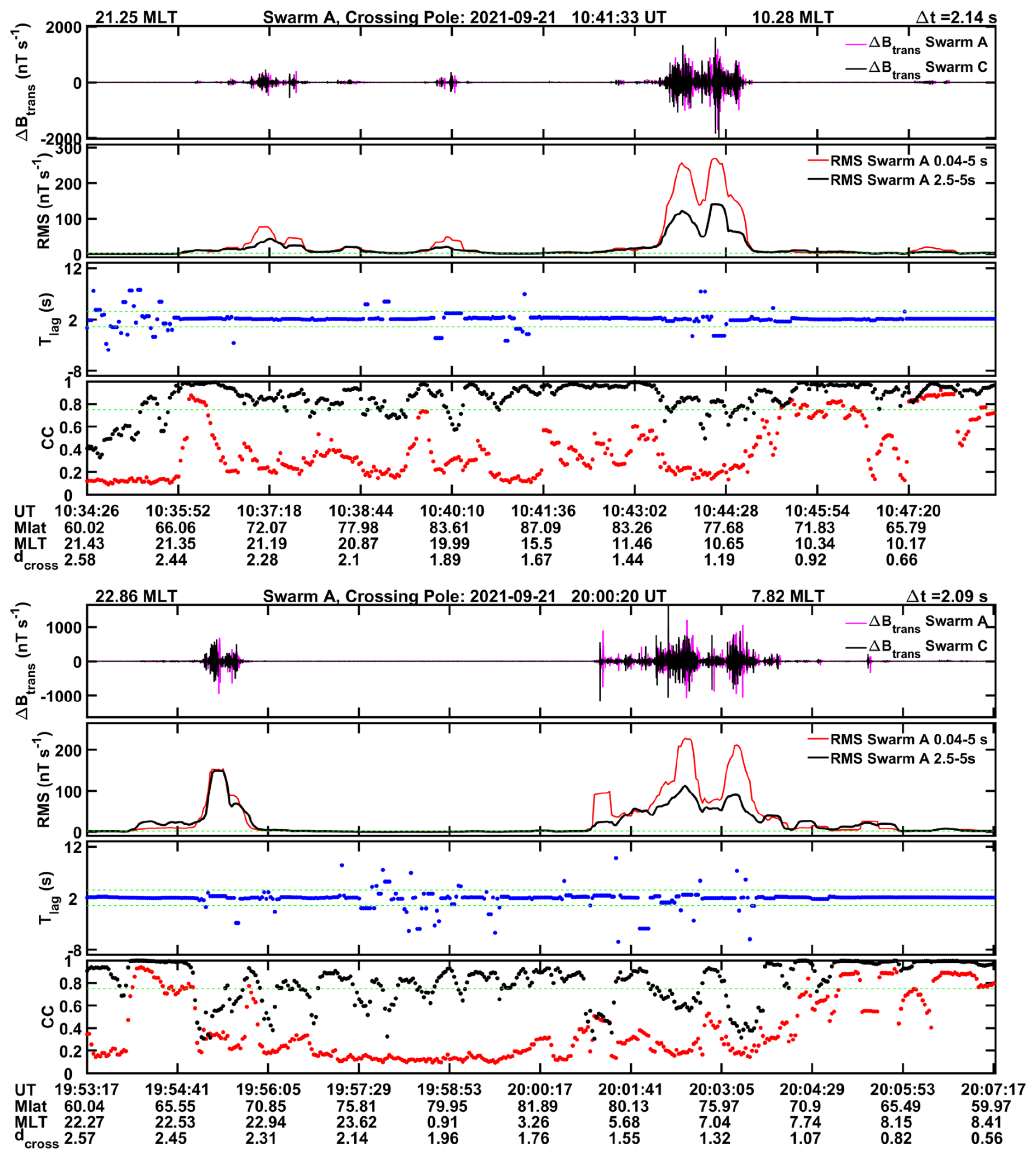
Figure 1 Examples of magnetic variations in the transverse, ΔB_trans, component within the period range of 0.04–5 s. The top panels of the two frames show the recordings of Swarm A and C along their orbits, crossing the polar region of the northern hemisphere. The second panels reflect the RMS value of the signal amplitude. Here the red curve shows the amplitude of the broad-band signal and the black curve that of the filtered 2.5 to 5 s period range. The latter values are multiplied by 5. The third panel contains the lag time, T-lag, between the signals for which the peak cross-correlation is achieved. The peak correlation coefficient, Cc, derived between Swarm A and C signals is shown in the bottom panels. Here again red dots result from the broad-band signal and black from long-period range. Along the horizontal axis temporal and spatial information is provided. The d_cross lists the spacecraft separation in cross-track direction.

From these observations we may conclude, that the longer-period signals reach largest amplitudes where broad-band signal appears. The cross-correlation coefficient between recording of Swarm A and C is reduced where the large-amplitude bursts occur, but it is still sufficient to deduce the optimal time shift from these long-period signals, fitting the actual along-track separation of Δt=2.1 s. On the other hand, the higher-frequency fluctuations are reaching only low Cc values, even at optimal time shift.

During both orbits, bursts of intense fine-scale features are observed with amplitudes surpassing partly 1000 nT s⁻¹ (corresponding to 100 µA m⁻²). They occurred predominantly in the morning and prenoon sector but also on the nightside, here less intense. Interestingly, the long-period amplitude follows closely the intensity of the broad-band signal (see second panels) but on a 5 to 10 times lower level. It may be surprising that the coefficient, Cc, is so low for the broad-band signal, although the cross-track spacecraft separation is only 1 km on the dayside and 2 km on the nightside, and the along-track time difference is only 2.1 s. Even more puzzling is the fact that the correlation coefficient for the long-period signals goes down in the regions where the FAC bursts appear. Answering these questions will be part of the study.

In order to get a better understanding of the small FAC characteristics, Fig. 2 shows for two bursts of activity a zoom into the magnetic signatures recorded by the two horizontal components, ΔB_trans and ΔB_along. Presented are intervals of 15 s, corresponding to about 100 km along-track. In the top frame observations from the late morning sector are plotted. Here, the recordings by the two spacecraft have little in common although the time-shift, Δt=2.1 s, between them has been accounted for. The lower frame is from the nightside. Also here, the signals at the two spacecraft differ significantly during active periods. Furthermore, when visually comparing the ΔB_trans and ΔB_along signals in Fig. 2, hardly any correlation is found between the two components lasting for some time. This indicates that the shape of the FAC structures is constantly changing.

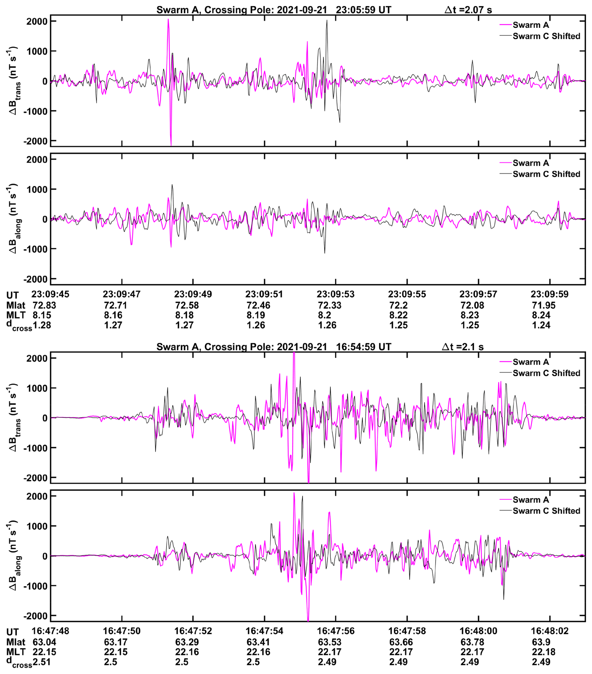
Figure 2 Examples of ΔB_trans and ΔB_along variations during bursts of km-scale FACs from the prenoon sector in the upper frame and from the nightside in the lower frame. Largest amplitudes are confined to very small scales. There is hardly any correlation observed between Swam A and C recordings.

The magnetic signature within the bursts covers a wide frequency spectrum. There is no clear preference for any frequency. Even very narrow features in ΔB_trans, e.g. around 23:09:48 and 16:47:55 UT, can reach large amplitudes. More details of the signal spectrum will be provided in Sect. 5.2. The FAC burst events in the upper and lower frames of Fig. 2 are from the day and night sides, respectively. Therefore, they are connected to very different source regions in the magnetosphere, but still, their characteristics are very similar. A pending question here is, what causes the fragmentation into the small filaments. By looking into a larger number of events we may find systematic characteristics.

4 Separation of the signal into period bands

From the examples presented above it is obvious that the FAC-related magnetic signal within the bursts covers a wide frequency range, and the variations of ΔB_trans and ΔB_along are quite independent from each other. Figure 1 furthermore suggests that the correlation properties between Swarm A and C vary with the apparent period (along-track scale length) of the signal. In order to identify the typical FAC properties we investigated the signal of the whole study period, 18 September to 4 October 2021, the days when the along-track separation was reduced to 2 s. Furthermore, we subdivide the signals of ΔB_trans and ΔB_along into eight quasi-logarithmically spaced period bands. The chosen −3 dB pass-band filter limits are 0.04–0.1 s, 0.1–0.16 s, 0.16–0.26 s, 0.26–0.44 s, 0.44–0.72 s, 0.72–1.2 s, 1.2–2.5 s, and 2.5–5 s. The last two period bands overlap with the spectral range of the FAC study by Lühr and Zhou (2025). In this way we want to extend that earlier study and find the relation between the km-scale and small-scale FAC characteristics. We interpret the apparent signal periods recorded by the satellites as along-track scale lengths of the current structures. Following the arguments of the earlier study we also here define halve the wavelength as the scale size of a FAC.

We have performed a cross-correlation analysis between the ΔB_trans components of the two satellites separately for the above listed period bands. For checking the stationarity of the signal, we applied the following analysis

$$\begin{array}{}\text{(2)}& \text{Cc}={\displaystyle \frac{\sum \left[\right(X-X_{\mathrm{m}})\cdot (Y-Y_{\mathrm{m}}\left)\right]}{\sqrt{\sum (X-X_{\mathrm{m}}{)}^{\mathrm{2}}\cdot \sum (Y-Y_{\mathrm{m}}{)}^{\mathrm{2}}}}}\end{array}$$

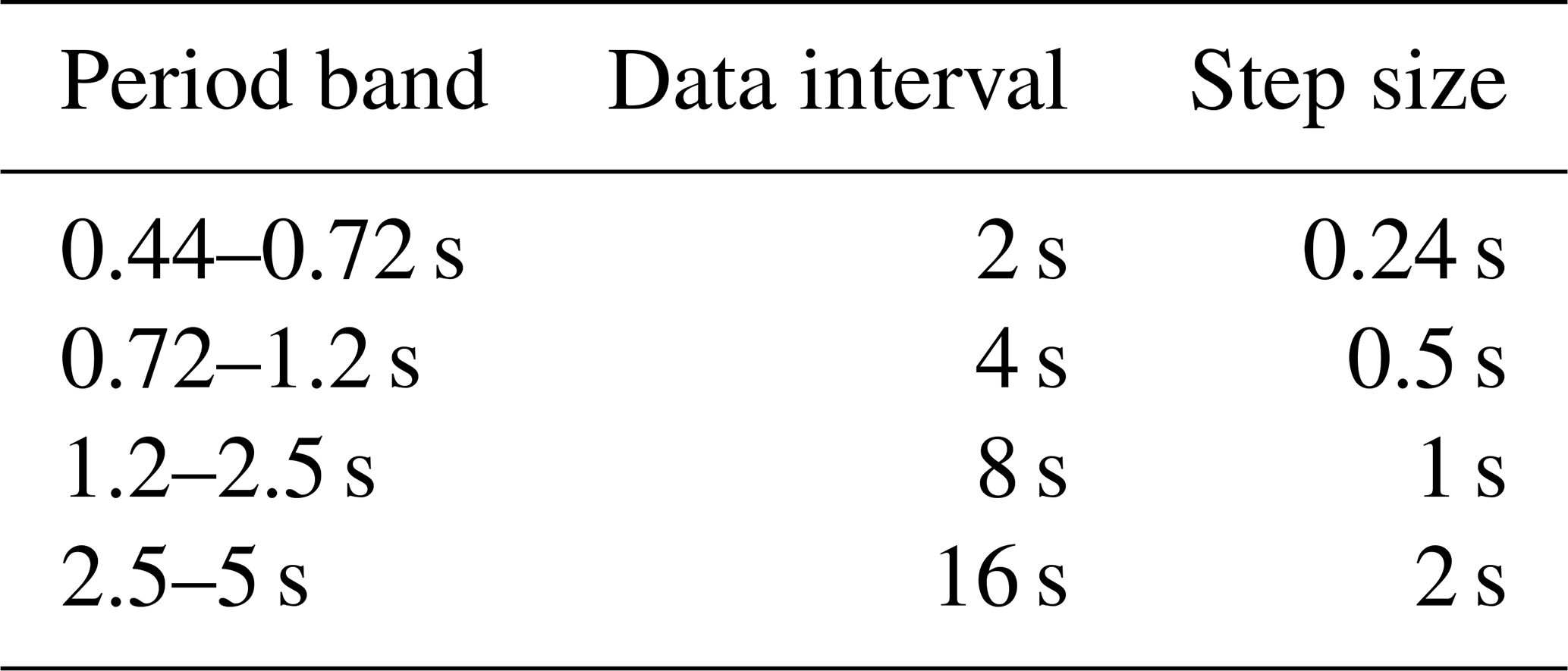
where, X represents the signal amplitude of ΔB_trans from Swarm A, Y represents the signal of ΔB_trans from Swarm C, and X_m and Y_m represent the mean values of ΔB_trans over the correlation intervals of the two satellites, respectively. The maxima of Cc and the corresponding time lags (T-lag) between the two satellite data series were determined. Applied data intervals and step sizes for the various period bands are listed in Table 1.

Table 1 Listing of the data interval lengths and step sizes for the cross-correlation analysis of the various period bands.

A number of criteria are defined for separating quasi-stationary FAC features from uncorrelated signal parts. The peak cross-correlation coefficient should be Cc>0.75 at a time shift close to the spacecraft separation time, Δt. It thus has to be T-lag=Δt ± 1.5 s. In order to make sure that only significant auroral FACs are considered, the signal variation, ΔB_trans, should surmount an amplitude threshold, RMS>2 nT s⁻¹. An equivalent set of criteria has been used by Lühr and Zhou (2025); therefore, direct comparisons between the two studies are possible.

A cross-correlation analysis has been applied to the signals in the four period bands listed in Table 1. Data intervals that pass all the above-described stability criteria are term “selected” and the others are “deselected”. Of interest here is the ratio of selected events normalized by all events (selected plus deselected) that exceed an amplitude of RMS=2 nT s⁻¹. Figure 3 presents for the northern (top) and southern (bottom) hemispheres the distribution of the derived ratios for the four considered period bands over the study period. Shown is the latitude distribution of the ratio, separately for each orbit, and for the up- and downleg arcs. White patches appear in Fig. 3 where no entries are available. Across the bottom of the frames we have listed the dates, magnetic local time (MLT) at 70° MLat, and the along-track time difference, between Swarm A and C. The up- and downleg orbital arcs are separated by about 12 h in local time. The displayed ratios cover the signal bands of apparent periods from 0.44 to 5 s (corresponding to 1.7–19 km scales).

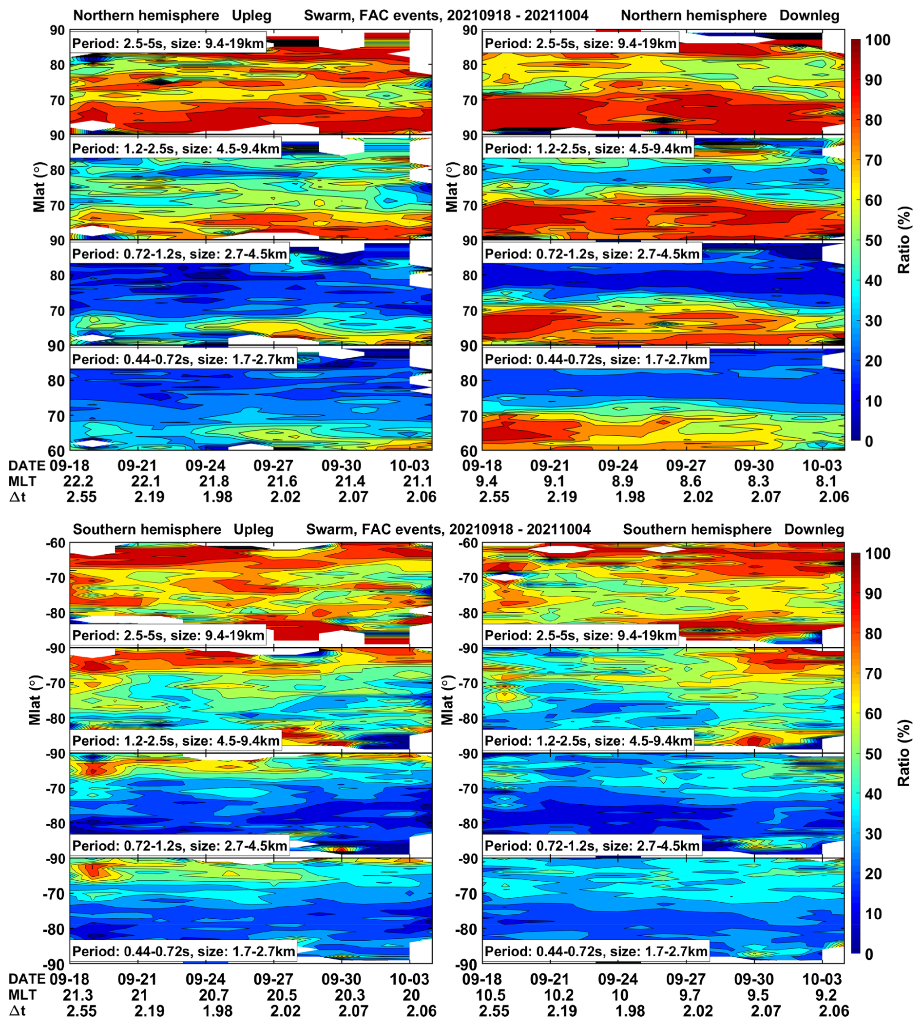
Figure 3 Latitude distribution of the ratio between positively detected stationary FAC structures and all wavy signals with amplitudes above the threshold of RMS>2 nT s⁻¹, separately for four period bands. Separate frames present up- and downleg orbital arcs, and the two hemispheres. The labels along the horizontal axis provide temporal and spatial information and the along-track time difference, Δt.

All four frames in Fig. 3 show an obvious change in correlation characteristic between the longest band (top panels) and the shorter periods below. A large majority (80 %–100 %) of the magnetic signatures in the 2.5–5 s period band (10–20 km scale) is well correlated between the two Swarm satellites. The smaller scale current structures (here 1.7–4.5 km scales) show much lower percentages of correlated features. Some exceptions are observed at the lower latitude end around 65° MLat, particularly on the dayside. This is especially true for the northern hemisphere and to a lesser extend to the nightside. For all the other regions and the shorter periods, the ratio of well-correlated events is low, typically below 20 %.

Here we like to mention that the cross-track separation between Swarm A and C is varying between 0.5 and 2.5 km during the 2 weeks of interest, while the along-track difference of 2 s is constant. When looking at the temporal evolution of correlation ratios in Fig. 3, we find hardly systematic changes following the cross-track separation. This observation strongly suggests that the decorrelation is dominated by the 2 s difference between quasi coplanar samples, not by the cross-track separation.

Quite outstanding are the high percentages of quasi-stationary FAC structures in the northern hemisphere for the longest period range, 2.5–5 s. This fact is valid for almost all latitudes except for a band between 75 and 80° MLat on the dayside and at somewhat lower latitudes on the nightside. The point of reduced correlation will be revisited in Sects. 5.2 and 6. On the other hand, hardly any well-correlated observations are found between Swarm A and C for periods shorter than about 1 s. This suggests, the FAC structures with along-track wavelengths of less than 7.5 km have a very short life-time, less than the 2 s, the lag-time between the sampling of the two satellites. It implies that the two Swarm satellites, even during this special constellation phase, cannot be used for estimating the FAC density of these narrow scales by means of the dual-satellite method (Ritter et al., 2013; Lühr et al., 2020). However, for the signals with periods longer than 2.5 s (>10 km scale) it can be used.

5 Statistical analysis

5.1 Polarization characteristic of FAC-related B-fields

When estimating FAC density from satellite magnetic field measurements a number of assumptions have to be made. This is in particular true when single-spacecraft measurements are interpreted. Most reliable results can be achieved when plane FAC sheets are crossed. In those cases, the two horizontal field components vary in phase. Conversely, when the satellite passes outside of the sheet or when the FAC has a filamentary shape, there exists a significant phase shift between the magnetic signatures of the two components. In those cases, FAC density estimates from single spacecraft are difficult.

In order to determine the magnetic signal properties, we analyzed their ellipticity parameters from the data of the two horizontal components, B_trans and B_along. For estimating the polarization parameters, we made use of the approach outlined by Fowler et al. (1967). In this way the following quantities are derived: the Ratio of polarized signal within the total signal, the degree of Ellipticity (a zero means linearly polarized, a +1 stands for right-handed circular and −1 for left-handed circular polarization), θ is the angle between the ellipse major axis and the B_trans component, f_peak reflects the frequency of the spectral peak within a given filter band, Amp_peak shows the signal amplitude at f_peak derived from the combined signal of the two components.

For the calculation of the ellipticity parameters we consider intervals of data that are twice as long as the longest period in a band and the step for successive processing is one quarter of the interval length. All these parameters are listed in Table 2 for the eight period bands. In this way we obtain a sufficiently detailed resolution of the signal variation at the various periods. The basis for the ellipticity analysis is the Fourier transform of the magnetic field recordings. We have considered for the further analysis, from each period band, only the four lowest frequency Fourier coefficients in the band (ignoring the constant part) because the higher frequencies fall beyond the filter cut-offs of the band-passes and represent mainly leakage effects. Just for the two longest period bands (1.2–2.5 s and 2.5–5 s) the five lowest frequencies are taken into account because of their larger bandwidth. The listed scale sizes signify halve the wavelength, as explained in the beginning of Sect. 4.

Table 2 Listing of the data interval lengths and step sizes for the ellipticity analysis of the various period bands.

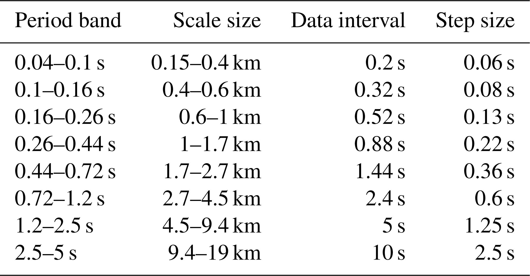
Figure 4 presents a compilation of the various ellipticity parameters and shows examples of comparisons with the actual data. Representative for the other filter bands, here the 0.16–0.26 s period range is selected. The analysis is applied to the active 2 s interval recorded by Swarm A on 21 September 2021, 23:09:47 to 23:09:49 UT. The signal context surrounding this bursty period can be seen in Fig. 6a. From the dynamic spectrogram in the top of Fig. 4a the limiting effect of the applied bandpass is clearly visible. Time-line plots of the two magnetic components exhibit largest amplitudes around 23:09:48.3 UT, as is also obvious from the spectrogram. In the frame below, the Ratio, in the bottom panel, stays close to 1, (except for a short period of small signal) indicating that the magnetic recordings can well be interpreted in terms of ellipticity for most of the time. The value of Ellipticity stays within ±0.2 for the one second around the signal peak, indicating a flat ellipse. Only during the first third of the interval is a more developed ellipse expected. These two regimes of Ellipticity exhibit also quite different angles between the ellipse major axes and the B_trans direction. Over the first third of the interval, we find large θ angles, up to 90°, while during the remaining two-thirds, small positive θ values dominate, implying a FAC sheet almost perpendicular to the orbit track. The spectral peak during this latter interval stays close to the frequency of 6 Hz, as expected for this filter band. The derived amplitude, Amp_peak (modulus of the combined B_trans and B_along) tracks well the signal intensity and reaches 20 nT around 23:09:48.3 UT.

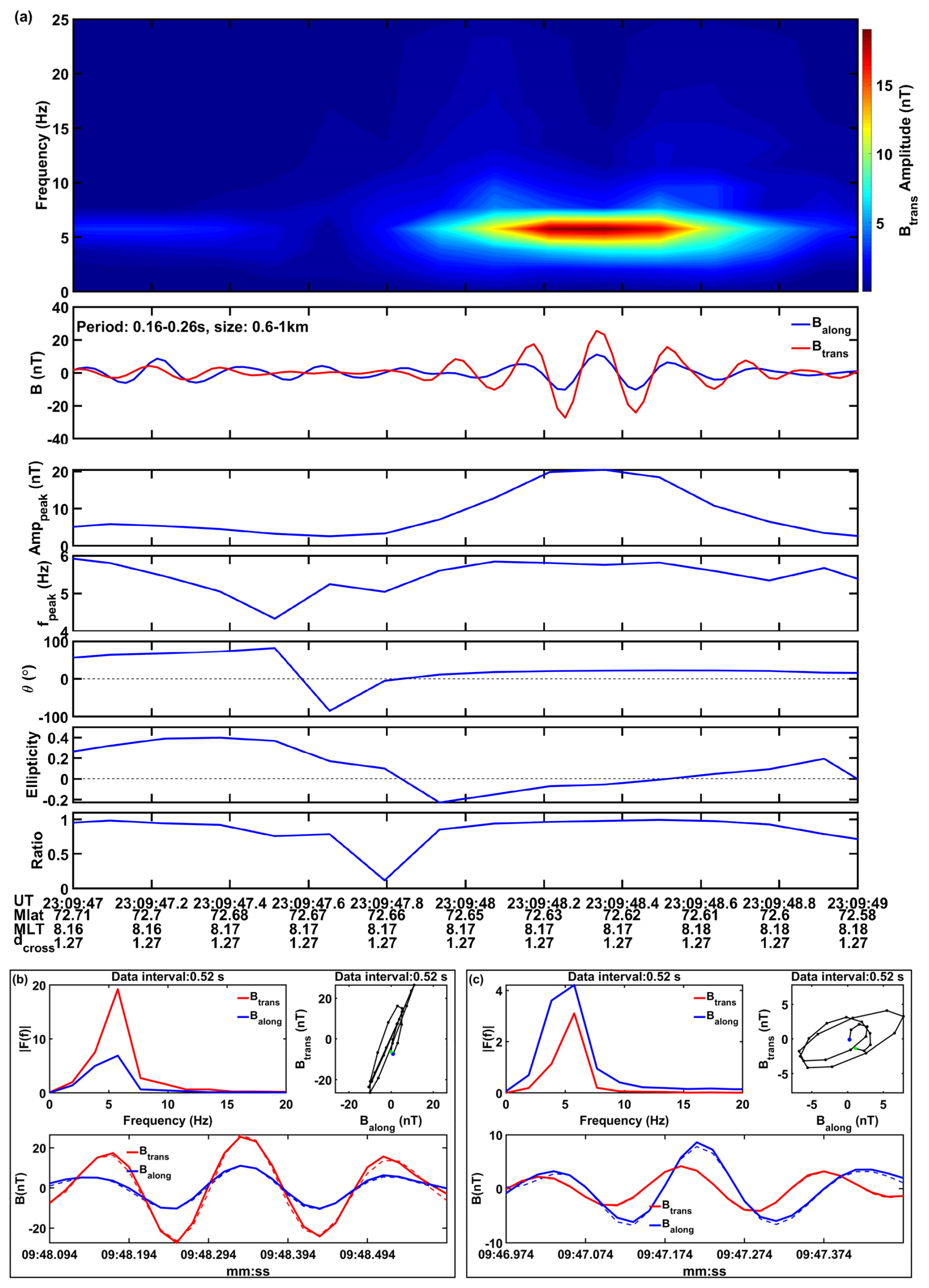
Figure 4 Example of ellipticity parameters derived over a 2 s interval for the 0.16–0.26 s period band. (a) The top panel displays the dynamic spectrum of the magnetic signal, below the time-lines of the two field components are shown. The five lower panels outline the temporal variations of the parameters determined by ellipticity analysis. (b, c) Details of the magnetic signals for two processing intervals.

The groups of panels in the lower part, Fig. 4b and c, show details of the results, taken along the line of processing steps, obtained from times of the two contrasting ellipticity regimes. In Fig. 4b, a time interval close to the signal maximum, the lower panels repeat the magnetic recordings of the two components. The dashed line represents the truncated spectrum and confirms that the four lowest frequencies, track the observed signals well. In the panels of the upper group, we find a nearly linearly polarized ellipse. Conversely, in the panels of Fig. 4c, derived from the early-time conditions, a clear phase difference exists between the magnetic field components. As a consequence, the hodograph shows a well-developed ellipse. All these derived ellipticity parameters will be used for estimating FAC densities at the various horizontal scales.

5.2 Deriving FAC density from ellipticity parameters

From the examples of magnetic field recordings, shown in Figs. 1 and 2, it is obvious that bursts of small-scale FACs with large amplitudes can be found both on the day and night sides. A question of interest is, are there preferred FAC scales sizes for the very large amplitudes? We thus tried to estimate the FAC densities separately for each period band. Due to the obvious filamentary shape of these small FACs there is no simple approach for obtaining reliable density values. Our chosen approach is thus to identify signatures of field variation that favor reliable FAC estimates.

The starting equation for commonly used FAC estimates from single-satellite magnetic field recordings is

$$\begin{array}{}\text{(3)}& j_z={\displaystyle \frac{\mathrm{1}}{{\mathit{\mu }}_{\mathrm{0}}}}{\displaystyle \frac{\mathrm{\Delta }B}{v_{\text{SC}}}}\end{array}$$

where ΔB is the time derivative, $\mathrm{d}B/\mathrm{d}t$, of the length of the vector formed by the components, B_trans and B_along, v_SC is the spacecraft velocity of 7.5 km s⁻¹, and μ₀ is the permeability in vacuum. Here, the crossing of a plane FAC sheet at right angle is assumed. In general cases there exists an angle, θ, between the sheet and the cross-track direction. Then the equation reads

$$\begin{array}{}\text{(4)}& j_z={\displaystyle \frac{\mathrm{1}}{{\mathit{\mu }}_{\mathrm{0}}}}{\displaystyle \frac{\mathrm{\Delta }B}{v_{\text{SC}}\cos \left(\mathit{\theta }\right)}}\end{array}$$

For the application of this equation to our small-scale FACs we make use of the ellipticity parameters. For example, the maximum magnetic field change within a given period band can be calculated from the derived peak amplitude and frequency

$$\begin{array}{}\text{(5)}& \mathrm{\Delta }{B}_{\text{peak}}=\mathrm{2}\mathit{\pi }{\text{Amp}}_{\text{peak}}{f}_{\text{peak}}\end{array}$$

Not all recorded wavy signals are suitable for FAC estimates. Therefore, we introduced 4 conditions for considering only the clean ones.

1. For obtaining clear ellipticity we require, Ratio>0.7.

2. Most reliable results are derived when the satellite crosses quasi-planar sheets of FACs indicated by near-linear polarization or a small Ellipticity value. We thus require, $\left|\text{Ellipticity}\right|<\mathrm{0.3}$.

3. In order to avoid problems from crossing the current sheet at too shallow angles, we require, $\left|\mathit{\theta }\right|<\mathrm{60}\mathit{°}$.

4. Very small signals, which may be caused by waves, are ignored by requiring, ΔB_peak>3 nT s⁻¹.

Figure 5a presents, as an example, for a 2 min interval of intense FAC activity (see Fig. 6a), the derived ellipticity parameters of the period band, 0.26–0.44 s. The five panels contain the derived values for the ellipticity parameters. Dashed horizontal lines in the panels mark the above-specified thresholds. Starting from the bottom, the Ratio is for most of the times above the limiting level of 0.7. The Ellipticity, in the panel above, is small during most of the interval and is thus suitable for FAC estimates. Also, the angle θ stays mostly inside the allowed range. In a majority of cases the angle is in the positive range. This is consistent with a FAC sheet nearly aligned with a circle of geomagnetic latitude. As expected, the spectral peak varies about the central frequency, 3.5 Hz, of the period band. Finally, the Amplitude closely tracks the signal activity shown in Fig. 6a. The ΔB_peak (see scale on right side) is calculated from the peak amplitude and peak frequency (see Eq. 5).

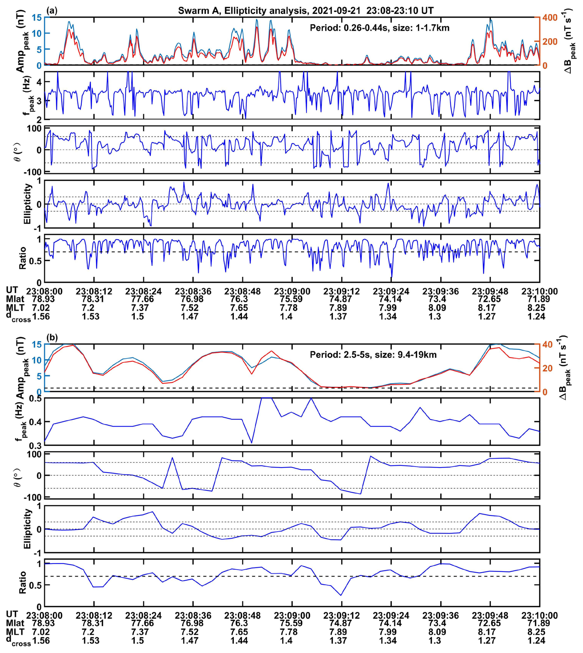
Figure 5 Temporal variation of the ellipticity parameters for a 2 min time interval. Dashed lines mark the thresholds that are considered for the estimation of reliable FAC densities. (a) Ellipticity parameters for the 0.26–0.44 s period band, (b) the same for the 2.5–5 s period band.

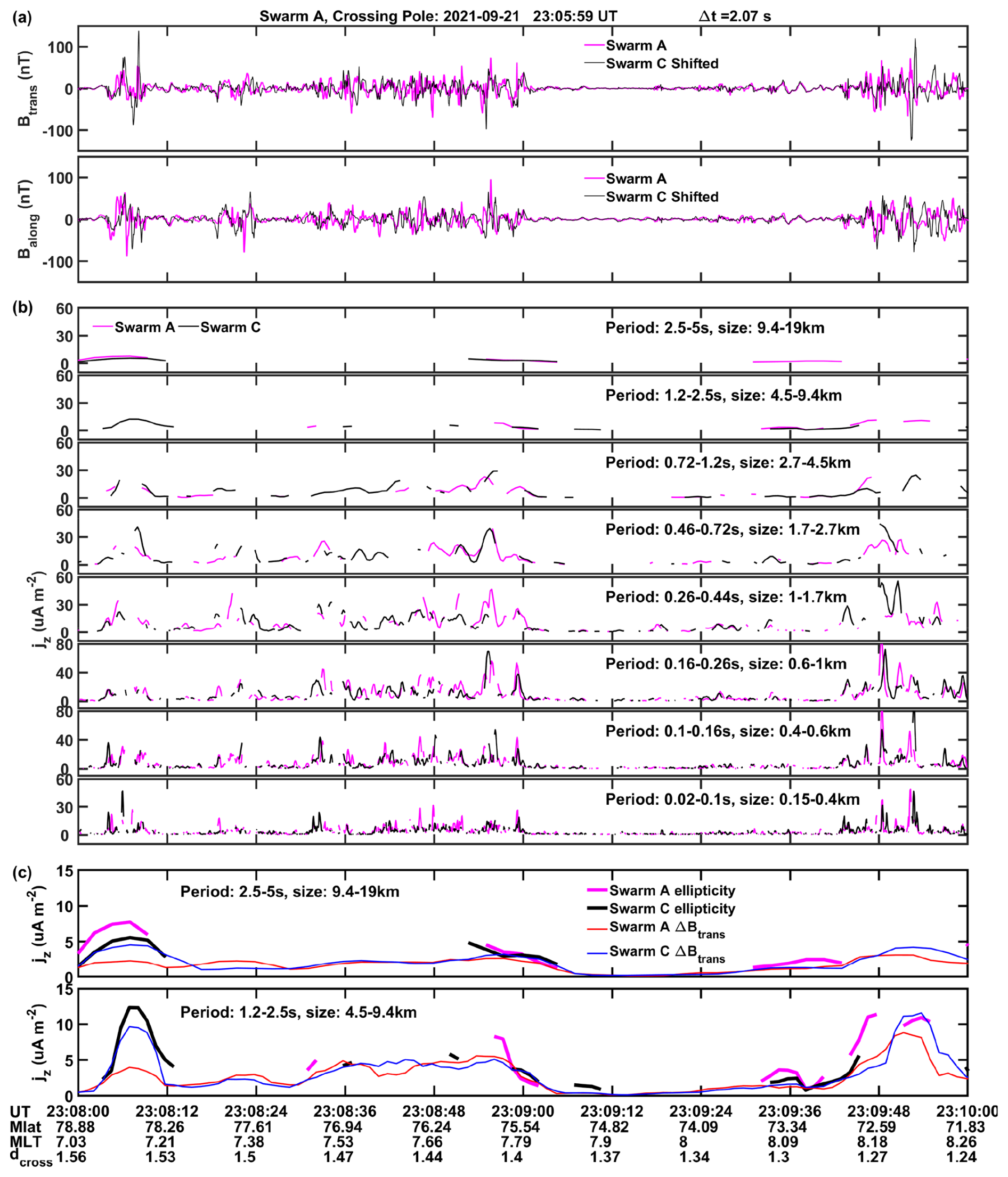
Figure 6 Temporal variation of FAC density estimates over a 2 min interval. (a) Timelines of B_trans and B_along variations over the considered interval, as recorded by Swarm A and C. (b) FAC density estimates derived from the ellipticity parameters, separately for all 8 period bands. (c) Comparison of FAC densities estimated by the simple single-satellite technique (thin lines) with results from the ellipticity approach (heavy line segments), for the two longest period bands.

For comparison, Fig. 5b shows the same set of ellipticity parameters but now for the longest period band, 2.5–5 s. The amplitude variations in the top panel track quite well the activity variations shown in Fig. 5a for the shorter-period signals. Otherwise, there are obvious differences. For example, the Ratio is on average lower, staying over longer periods close to the threshold. This indicates the presence of inharmonic signals, not contributing to the ellipticity. The Ellipticity, in the panel above, attains in several cases of sufficient Ratios large values outside the allowed band. For the angle θ we obtain again predominately positive values. The spectral peak is found around 0.4 Hz (2.5 s period) at the upper boundary of the period band. Worth noting is the difference in ΔB_peak, the scale range is smaller by a factor of 10 than that of the 0.26–0.44 s period band. This confirms also here a rapid decrease of FAC peak amplitudes towards larger structures.

With this information at hand, we can estimate the FAC density wherever the ellipticity parameters stay within the allowed ranges. Figure 6a presents the magnetic variations of the 2 min interval taken as an example. It is the same as considered in Fig. 5. In Fig. 6b we show the derived FAC densities for all the 8 period bands. Both the results from Swarm A and C are plotted. Since Swarm C sampled the same region 2 s later, its data series can be considered as independent from Swarm A. As can be seen in Fig. 6b, the current estimates from the two spacecraft complete each other quite well for the period bands shorter than 1 s. Thus, for them a fairly complete coverage is achieved. Times of enhanced and reduced FAC activity can well be tracked through all periods.

Just for the two longest periods fairly large gaps appear between valid FAC estimates. We have looked into the reasons for the gaps by checking the ellipticity parameters. Starting with the 2.5–5 s period band, in total 48 values are expected from Swarm A. From them 37 did not pass all the checks. Reasons were in 24 cases too large Ellipticity, in 20 cases too large angle θ and 17 times too small Ratio. As is obvious from the sum of these listed cases, two of the violations often occurred at the same time. Here a large Ellipticity was frequently accompanied by a large θ. Similar reasons have been deduced for the gaps in FAC density curves of the 1.2–2.5 s period band. These results indicate that field-aligned currents in the period range longer than 1 s (>5 km scales) are preferentially organized in filaments rather than current sheets.

It is interesting to note that the FAC peak amplitudes vary with the period (scale size). When looking at the panels of Fig. 6b, we find small current density values for the shortest period. The value increases rapidly towards the period band of 0.16–0.26 s. Largest FAC peak densities are observed in the 0.16–0.44 s period range (0.5–1.5 km scale size) reaching values up to 60 µA m⁻². For longer periods the amplitudes drop again. In the 2.5–5 s period band peak values are already down by about a factor of 5.

For verifying our FAC density estimates we performed for the period bands 1.2–2.5 s and 2.5–5 s a comparison with the densities derived by the basic single-satellite approach, as given in Eq. (3). Although these bands are least likely to be linearly polarized, so Eq. (3) may not be very accurate for FAC estimates, we made use of the ΔB_trans for ΔB in Eq. (3). The two panels of Fig. 6c show RMS values of the FAC densities as continuous curves from Swarm A and C, derived by the classic approach. For comparison, the partly available FAC densities from our ellipticity approach are added as heavy line segments. In principle, similar values are achieved by the two methods. It is expected that the ones from ellipticity are larger because they report the peak amplitude while we have shown the RMS values from the basic approach. It is convincing to see that the two very different techniques of FAC estimates provide quite similar results. Both methods confirm the reduction of FAC amplitudes towards longer periods (larger scales).

For supporting our suggestion of filamentary small-scale FAC structures we made some simple model calculations. As outlined by a cartoon on the left side of Fig. 7, we assume a fluxtube with circular cross-section of radius, r=10 km. For four satellite tracks past the tube center at distances e=20, 7, 5, 1 km we calculate the B_trans and B_along variations when assuming a current strength I=1 kA and homogeneous current density distribution within the fluxtube. The four hodographs in Fig. 7 illustrate the ellipticity characteristic of the derived field variations. It is obvious that we obtain in most cases well developed ellipses and an almost linear relation between B_trans and B_along only when passing close to the center. The artificially looking constant levels of B_along are from the passage through the current tube. If we had assumed a more realistic current density distribution that decreases from the center towards the border, the hodographs would have been even more elliptic. In any case, from these four example passes, only the last one, passage close to the center, would have passed our criteria for FAC estimates. This is consistent with our sparse yield of FAC estimates from the longest period band.

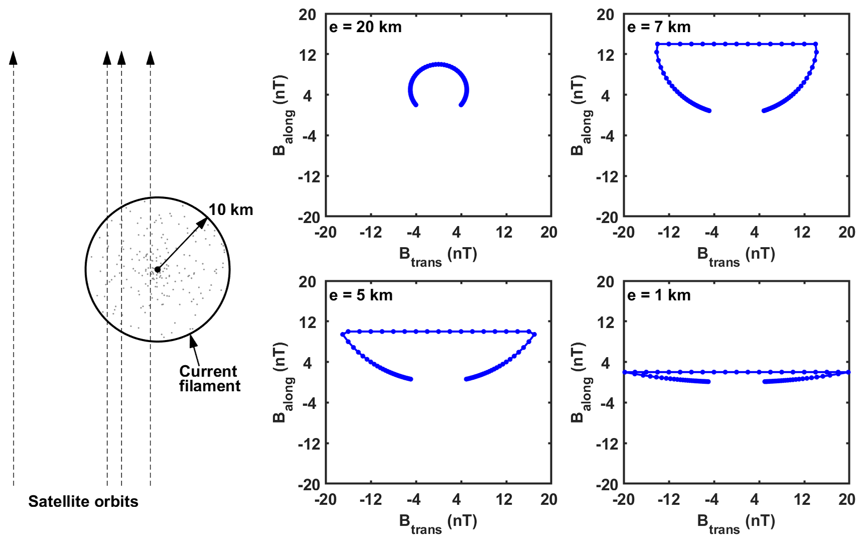
Figure 7 Modelling of the magnetic field ellipticity signatures for passes by a circular current tube of 10 km radius. On the left side the considered 4 trajectories at different distances past the current tube are illustrated. Resulting hodographs of the expected field variations are shown on the right side. Constant values of the B_along components come from measurements inside the tube with a homogeneous current density distribution.

So far, we looked only at short data intervals. For obtaining a better impression of the km-scale FACs we have plotted the derived FAC peak densities over the whole study period, 18 September through 4 October 2021. Results from Swarm A and C are again combined. Figure 8 shows the latitude distribution of derived peak current densities from each orbit for the five period bands, covering the period range, 0.1–1.2 s (0.4–4.5 km scales). The shortest period band has been dropped because of the fairly small amplitudes, and the two longest periods are not shown because of their sparse yield of reliable FAC estimates.

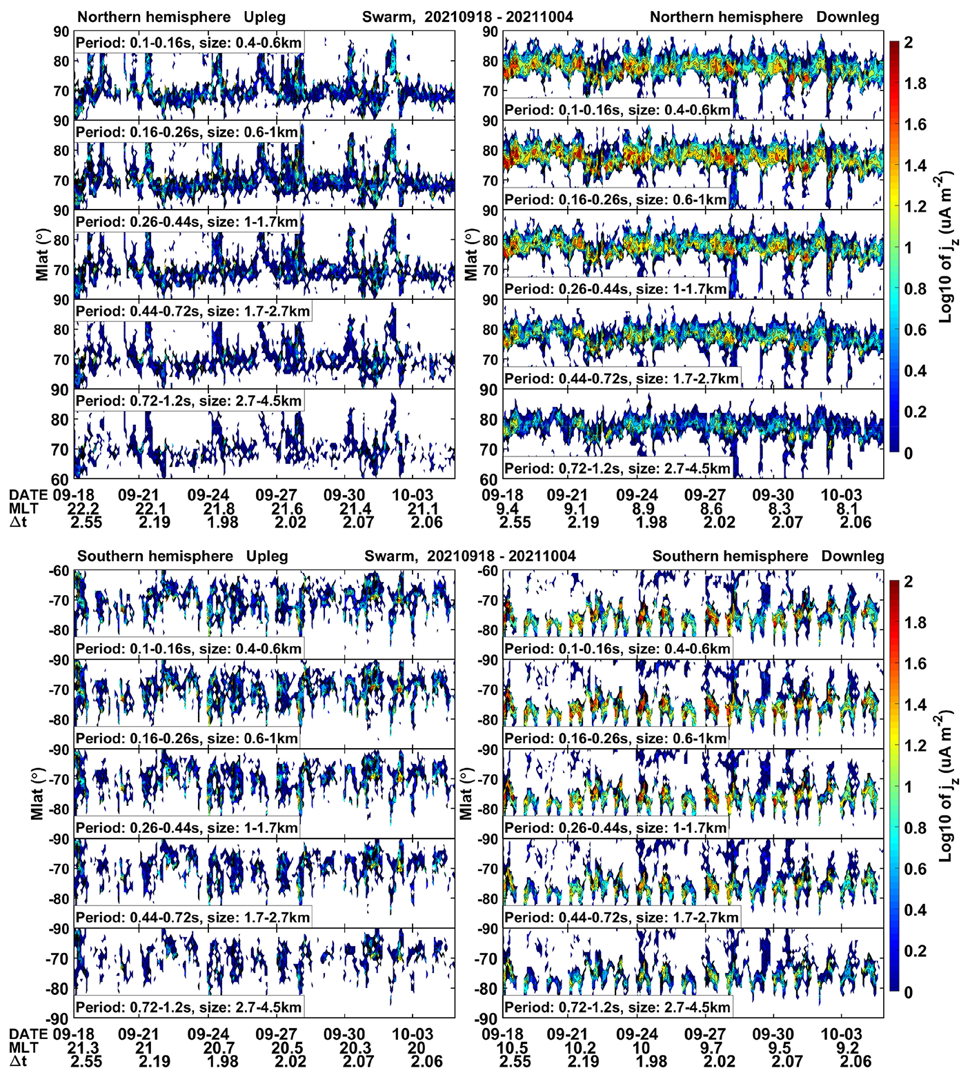
Figure 8 Latitudinal distribution of km-scale FAC density for the five period bands with largest amplitudes. The format is the same as that of Fig. 3, but only structures of horizontal scale sizes between 0.4–4.5 km are shown. White areas mark ranges without entries.

Figure 8 presents in the top row results from the northern hemisphere. The bottom row shows FAC densities from the southern hemisphere. The left column depicts km-scale FAC activity in the late evening sector around 21:00 MLT, which is close to the typical local time for substorm onsets (22:00 MLT) (see Wang et al., 2005) and to flow burst activity in the magnetotail (see Angelopoulos et al., 1994). The right column shows FAC activity in the prenoon hours. Because of the large range of derived FAC densities, a logarithmic scale has been chosen for the color bar. From both time sectors and over the whole study period we find clear evidence that largest FAC densities, up to 100 µA m⁻² are observed around the period range 0.16–0.26 s (0.6–1 km scale size). For longer periods the peak amplitudes drop significantly or fall even below our amplitude threshold.

Commonly, the km-scale FACs occupy only narrow latitude ranges of the auroral region, which vary with local time. In the prenoon sector, right column, this range is found at the poleward border, around 80° MLat, in the cusp/cleft region. Only occasionally signals are detected down to 60° MLat. In the southern hemisphere, regularly appearing gaps of current density are observed in the prenoon sector. They are caused by the fact that the Swarm A/C orbits in certain longitude sectors do not reach sufficiently high magnetic latitudes in this hemisphere. The extension of FAC activity to lower latitudes is achieved at similar UT times every day in both hemispheres. In the left column of Fig. 8, the pre-midnight km-scale FACs appear predominantly in the auroral oval around 70° MLat. This is the typical latitude for substorm activity and flow burst activity in the magnetotail. Also here, on certain days the activity extends to high latitudes. The appearance of FAC activity over a wide latitude range is an orbital effect. On most orbits the Swarm satellites approach the auroral region on their upleg arc around late evening and pass over through midnight to the morning sector. But due to the displacement of the magnetic pole, in some longitude sectors the passage goes from evening via noon sector to the morning side. In those cases, the plots in the left column contain also some noontime activity at high latitude. Similarly, the right columns contain some orbit-related duskside signal at lower latitude. Generally, in the southern hemisphere the FAC activity is not so well confined in latitude as in the north. This is caused by the larger offset between magnetic and geographic poles in the south. Thus, the MLT and MLat coverage by Swarm is varying much more between orbits in the southern than in the northern hemisphere.

When looking at km-FAC densities, the peak amplitudes, averaged over 1° in latitudes, vary on the dayside typically around 10 µA m⁻² but occasionally reach up to 100 µA m⁻². In the pre-midnight sector these peak averages are about an order of magnitude smaller. This confirms earlier results that intense, km-scale FACs appear most often in the sunlit high latitudes, particularly in the cusp/cleft region.

The previously shown results have identified the apparent period range 0.16–0.44 s (0.6–1.7 km scale) as the one where FAC densities peak. Now it would be interesting to see the spectral distribution of FAC density during times of enhanced activity. Figure 9a presents, as an example, a 5 min segment from 30 September 2021 of a pass through the cusp/cleft region in the southern hemisphere, which comprises a rather long passage through a region of intense small scale FAC activity. Shown are the ΔB_trans and ΔB_along components from Swarm A and C. Fluctuations reach up to 2000 nT s⁻¹. The interval from 23:41:30 to 23:44:00 UT is used for a harmonic analysis. Resulting spectra from the two components are presented in Fig. 9b. Here the spectral amplitudes have been averaged over a half-octave frequency range, in order to enhance the significance of the amplitude curve. Furthermore, the spectral results from Swarm A and C have been combined. A quite obvious spectral feature of both curves is the steep drop in signal strength towards lower frequencies. This is caused by the high-pass filter with a cutoff period at 5 s (see vertical dashed line). The spectra from the two magnetic field component, ΔB_trans and ΔB_along, exhibit very similar shapes but the spectral amplitude from ΔB_trans is larger by a factor of about 1.5 than that of ΔB_along. This indicates that the FAC sheets are preferentially aligned along circles of magnetic latitude.

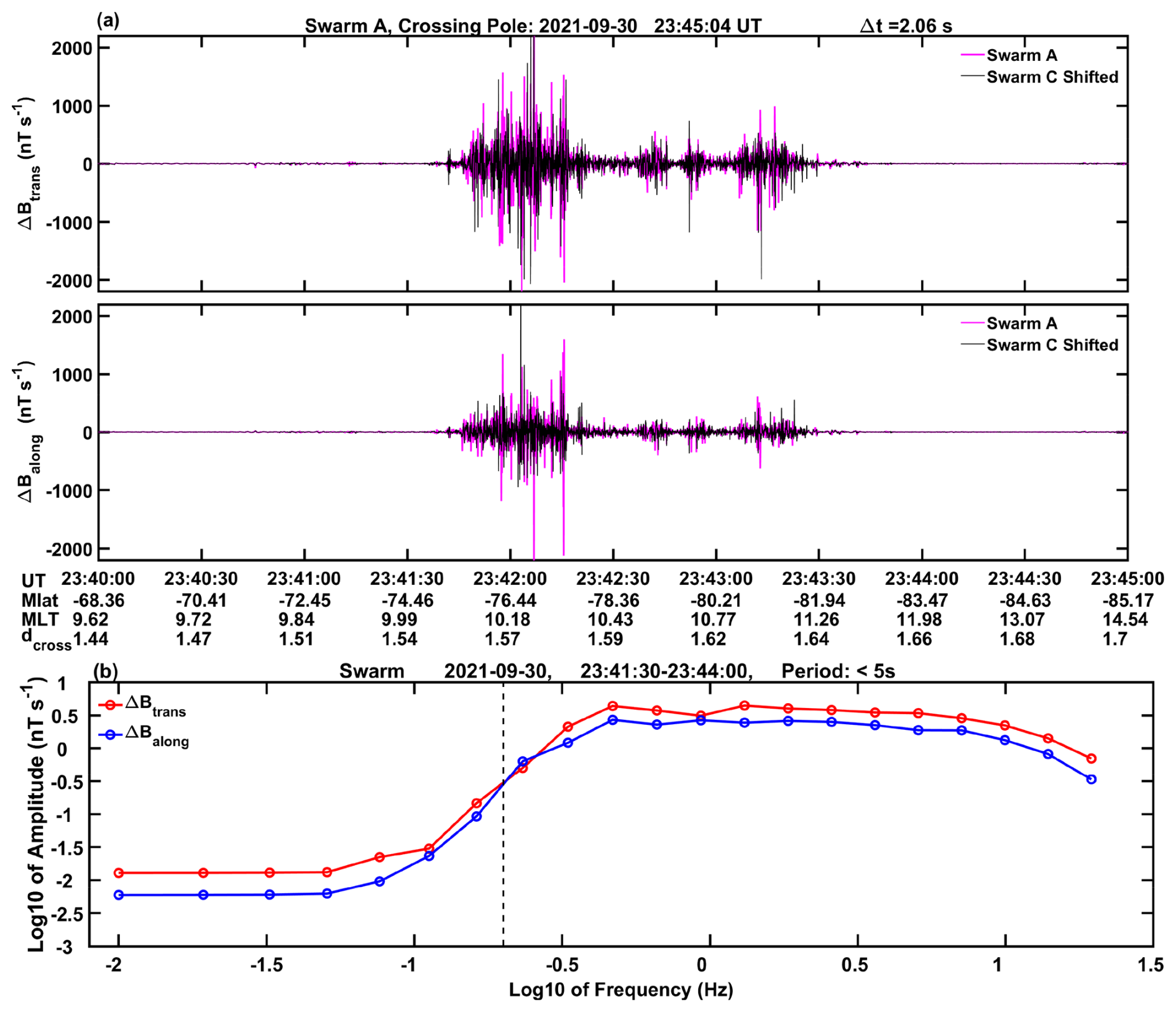
Figure 9 Example of signal spectra for a typical burst of km-scale FAC activity, separately for the field components ΔB_trans and ΔB_along. The steep amplitude roll-off is caused by the applied high-pass filter with a cutoff at 0.2 Hz (vertical dashed line). Spectra from Swarm A and C have been averaged.

Over the main part of the covered frequency range, we find a rather flat spectrum. Just at the high-frequency end, beyond about 8 Hertz, it starts to roll off. This is consistent with our observation of smaller FAC amplitudes within the shortest period band (0.04–0.1 s, 0.15–0.4 km scale). On the other hand, we find in Fig. 6 also FAC amplitude decreases towards the long-period end, a trend which is not reflected by the spectra. Obviously, the spectral shape is governed by the randomly appearing narrow large FAC spikes. They are causing an almost white spectrum reaching far into the lower frequency region. In that way they seem to override the contributions of longer-period signals to the spectrum.

6 Discussion

The focus of this study is on the km-scale FACs. However, we have included here also a part of the small-scale FACs with scale sizes of 5 to 20 km. These small-scale FACs were at the center of interest in our recent paper, Lühr and Zhou (2025). By using the high-resolution magnetic field data with a sampling rate of 50 Hz, here we extend the previous study to the smallest FAC scales resolved by the Swarm magnetometers. Furthermore, the previous investigations already indicated that there might be a connection between the two classes of FAC structure, but actually the two classes exhibit rather different characteristics. The km-scale FACs are made up of randomly occurring intense current density spikes. As a consequence, an almost “white spectrum” is obtained from the harmonic analysis of the magnetic field variations (see Fig. 9), reaching far into the longer period range. These spectral features are consistent with the results of Rother et al. (2007) who investigated kilometer-scale FACs based on 5 years of CHAMP data. They also report a flat FAC amplitude spectrum with a high-frequency role-off starting at 8 Hz. They argue that very intense narrow FACs appear randomly and with a spectrum exhibiting a long tail towards lower frequencies. The tail overlaps with the signals from the longer-period FAC structures. The upper cut-off frequency is determined by the typical width of the largest spikes, about 1 km (7.5 [km s⁻¹]$/$8 [Hz]), as reported by Rother et al. (2007) and found here. The good agreement with their more comprehensive statistical study suggests that our single spectrum result represents typical features of the km-scale FACs.

The km-scale FACs are limited to certain latitude regions that vary with local time. Individual features are very variable, lasting only order of 1 s. When visiting the same location 2 s later, structures with comparable amplitudes are seen but with quite different waveforms. Largest FAC densities are found for horizontal scale sizes of 0.5–2 km.

Conversely, the small-scale FACs reported in our previous study were found to be stationary over about 18 s. They exhibit a longitudinal correlation length of about 12 km and occur over a wide range of auroral latitudes. Whenever the small-scale FACs are accompanied by intense km-scale current structures their correlation properties between the recordings at the two Swarm satellites are compromised. This can directly be seen in the example displayed in Fig. 6a. The magnetic field recording of Swarm A and C are indistinguishable during times without km-scale features (e.g. 23:09:00–23:09:40 UT). But tiny small-scale structures are also present here. When FAC bursts appear, the small-scale signal is distorted but has larger amplitude. A confirmation of these characteristics can be obtained when comparing Figs. 3 and 8. The ratio of well-correlated small-scale FACs (2.5–5 s period) in Fig. 3 ranges around 90 %, except in some latitude bands. Intense km-scale FAC activity occurs on both the dayside and nightside in these same latitudinal bands in Fig. 8. We regard this effect as a consequence of spectral leakage from the km-scale into the small-scale FAC signal range.

In spite of the listed differences between the characteristics of the FAC classes, there seems to be a close relationship between them. Already in Fig. 1 we showed the juxtaposition of the superimposed scales. Whenever the amplitude of the broadband signal increases, the long-period signal (2.5–5 s) follows that trend although reduced by a factor of 5 to 10. A part of the signal strength in the low-frequency range may come from the broad-band contribution, but the fairly stable estimates of a correct T-lag imply a sufficient strength of the true small-scale FAC signature. Although the cross-correlation coefficient, Cc, of the small-scale variations drops simultaneously with the appearance of the intense km-scale signal, it still finds its maximum at the right time shift. Reduced Cc values at other locations, not accompanied by km-scale features, are caused by the very low signal amplitude of the small-scale signal. The observations of km-scale variations only appear in connection with a small-scale FAC signal, and small-scale FACs reach largest amplitudes only in regions where also km-scale signal appear. Already Lühr and Zhou (2025) found that large-amplitude, small-scale FACs exhibit reduced cross-correlation in the presence of more greatly amplified km-scale signals. These latter findings strongly suggest a connection between the simultaneous appearance of amplified small- and km-scale FACs.

For an explanation of that connection, we should have a closer look into the characteristic of the small-scale FACs. For example, Park et al. (2017) made use of Swarm electric field and magnetic field data to determine the reflection properties of the ionosphere for Alfvén waves in the period range from 2 to 15 s. This range overlaps very well with our class of small-scale FACs as defined in Lühr and Zhou (2025). Due to limitations of the E-field instrument on Swarm, Park et al. (2017) could not examine all seasons and local times, but for equinox conditions in 2014 they present a fairly complete picture. The September, October 2021 dataset considered here is also near equinox. Park et al. (2017) derived the wave reflection coefficient, α. The value α=0 indicates a complete absorption of the wave in the ionosphere, hence no reflection. Conversely, α=1 is expected for a perfectly conducting ionosphere which would produce total wave reflection. From the relation between E- and B-field perturbations they confirmed that the variations within their selected period range act like Alfvén waves. Park et al. (2017) reported largest reflection coefficients around 75° MLat on the sunlit dayside and around 65° MLat on the dark nightside with values of α=0.3–0.5. This indicates significant wave reflection in the region where we observe the small-scale FAC bursts.

It is well established that Alfvén waves can oscillate between the ionosphere and a magnetospheric reflection layer to form an Alfvén resonator (e.g. Lysak, 1991). There are also other Alfvén resonators described in the literature, e.g. the ionospheric Alfvén resonator (IAR) (e.g. Lotko and Zhang, 2018), which is confined to F-region altitudes. We prefer the one formed by the conducting ionosphere at the low-altitude boundary and the outward gradient in Alfvén speed at higher altitude, of order 1 to several R_E. Large-amplitude km-scale FACs have also been observed by the Freja satellite at 1700 km altitude in the cusp region and nightside auroral oval (e.g. Lühr et al., 1994). More recent studies show that counter-propagating Alfvén wave packets nonlinearly generate wave components at shorter wavelengths and higher frequencies (e.g. Maron and Goldreich, 2001; Chandran, 2004). When the interaction proceeds for a sufficiently long time, the resulting magnetic field fluctuations become turbulent. We suggest that this process occurs in the latitude regions where bursty signals are observed. It requires, however, continuous input of wave energy to compensate for losses due to ionospheric collisional dissipation. In the stationary state the obtained amplitude is determined by the balance between input power and dissipative losses. Greater input power yields larger amplitudes.

For further testing the idea of turbulent interaction we determined the power spectral density (PSD) of the magnetic field fluctuations. As an example, we took again the km-scale FAC burst on 30 September 2021 around 23:42 UT, shown in Fig. 9. The PSDs of the fluctuations from the two horizontal magnetic field components have been added. For enhancing the significance of the spectrum, the two very similar results from Swarm A and C have been merged and then averaged over a half-octave frequency range. Figure 10 presents the resulting PSD curve on log-log scales. In this case no high-pass filter has been applied to the data. The well confined interval of bursty signal is just detrended. Towards higher frequencies the PSD follows a power law decay. Over a large frequency range the spectral index equals $-\mathrm{5}/\mathrm{3}$. Such a slope is expected for fluid turbulence. This so-called Kolmogorow spectral slope is add for reference (dashed blue line). At frequencies beyond about 3 Hz the decline becomes steeper. We like to interpret our steeper decline as an indication of enhanced power dissipation during the process of turbulent interaction. This dissipation obviously increases a lot for signals with apparent frequencies larger than 8 Hz (wavelength <1 km).

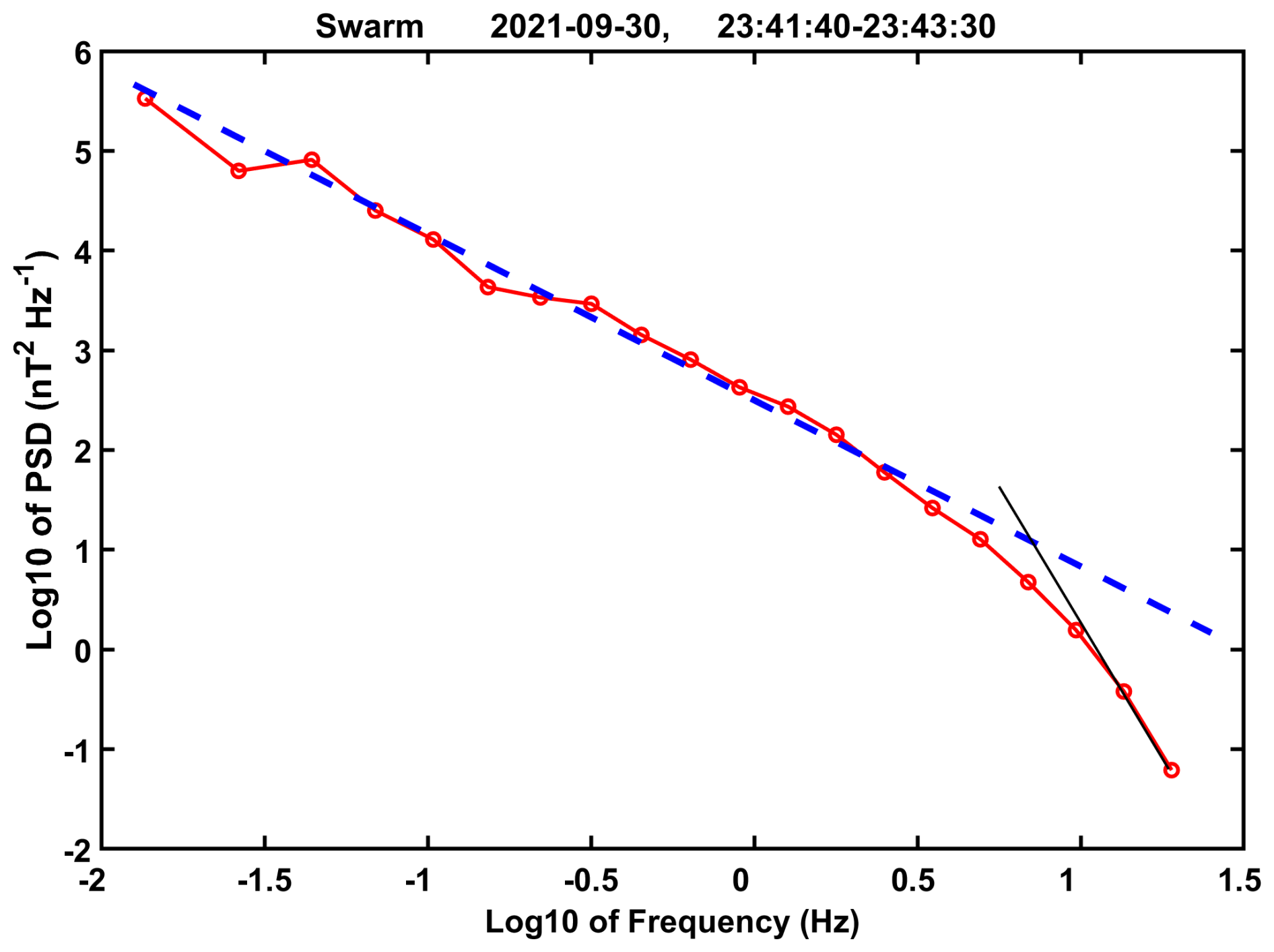
Figure 10 Power spectral density (PSD) of the magnetic field variations observed during the FAC burst shown in Fig. 9a. No filter has been applied in this case, and the PSDs from the two horizontal components are added. Spectra from Swarm A and C have been averaged. The dashed blue line represents the slope of the Kolmogorow index, $-\mathrm{5}/\mathrm{3}$, which is typical for fluid turbulence.

Throughout the paper we have interpreted temporal variation, recorded by the satellites, as crossings through spatial structures, but in reality, we cannot separate between temporal and spatial variations. The observed Doppler shifted magnetic field observations can be expressed as

$$\begin{array}{}\text{(6)}& B=A\cos \left[\right(\mathit{\omega }+vk\left)t\right]\end{array}$$

where A is the amplitude, ω is the cycle frequency, v is the spacecraft velocity, t is time, k is the wavenumber component in flight direction. Due to the large spacecraft velocity, the second term always dominates. Even for the smallest structures (<0.5 km), which are shown to be highly variable, we think the second term is about 10 times larger than the ω. All this shows that the interpretation of apparent signal variation as spatial scale is justified, but the resulting scale sizes are slightly underestimated.

The power loss scales as 1−α², so the Park et al. (2017) study with reflection coefficients of α=0.3–0.5 for small-scale Alfvén waves indicates that most of the Alfvén wave power (75 %–90 %) is dissipated in the ionosphere. This finding assumes, however, that the primary dissipation process is Joule heating. For km-scale Alfvén waves, the dominant dissipation process is Ohmic heating due to the finite parallel conductivity of the ionosphere (e.g., Lessard and Knudsen, 2001). The turbulent interaction between oscillating Alfvén wave packets is transferring energy from longer to shorter scale-length. Thus, the km-scale FACs gain more in amplitude than the small-scale FACs inside the activity bursts, which is consistent with our observations. However, Lessard and Knudsen (2001) also state that Alfvén waves below a certain spatial size are strongly damped upon traversing the ionosphere. Furthermore, the km-scale structures also seem to exhibit higher harmonic frequencies (>0.5 Hz) in the Alfvén wave resonator. This can explain the observed decorrelation between signals that are sampled only 2 s apart.

A remaining question is, what determines the smallest FAC sizes. The quasi-white spectrum starts to roll-off at an apparent frequency around 8 Hz. The corresponding 1 km wavelength can be regarded as the smallest wavelength of these bursty FACs. In a relevant model study, Lotko and Zhang (2018) have investigated the ionospheric dissipation properties of short-wavelength Alfvén waves trapped in an ionospheric Alfvén resonator formed by the plasma density gradients of topside and bottomside F-region. As expected, for longer wavelengths (>20 km) and lower frequencies they find the largest Joule heating rates in the E-region. For shorter wavelengths and, in particular, for higher harmonic resonator modes, dissipation in the F-region becomes increasingly important and severely limits the amplitudes of sub-km-scale modes. The resulting ionosphere-thermosphere heating at F-region altitudes, predicted by their model, is well supported by the observations of local air upwelling in connection with km-scale FACs in the cusp region (e.g. Lühr et al., 2004). In addition, these authors point out that single-satellite recordings of small-scale Alfvénic structures suffer from the spatial/temporal ambiguity when flying through regions containing very small-scale and multi-harmonic, F-region resonator modes. Thus, quantitatively determining detailed properties at the smallest scales is difficult from Swarm observations. Lotko and Zhang (2018) also note that absorption at wavelengths <0.5 km, projected to the F-region, occurs at altitudes above 2000 km where wave-particle interactions due to electron inertial effects and attendant Alfvénic parallel electric fields produce the soft (broadband) electron precipitation that commonly accompanies bursts of km-scale FACs (e.g. Watermann et al., 2009).

These considerations offer useful insights into the Swarm observations of km-scale FACs, but with some limitations. None of the ionospheric Alfvén resonator models address polarization characteristics, so we are left without an explanation for the transition from the magnetic elliptic polarization of small-scale FACs to the near-linear polarization of km-scale FACs. Alfvén waves do change helicity upon reflection at a conducting surface, so ionospheric reflection may produce a nearly linearly polarized superposition of right and left hand elliptically polarized waves above the E-region. Existing models are also linear or two-dimensional and cannot describe the generation of turbulence leading to the shorter wavelength and higher frequency wave power of km-scale FACs. While we have identified a possible causal connection between small- and km-scale FACs, how power in the energy-containing small-scale FACs cascades to the observed km-scale FACs remains unresolved.

7 Summary and conclusion

In this study we investigated the characteristics of the smallest-scale field-aligned currents at auroral latitudes. For this purpose, we used the high-resolution magnetic field data sampled at 50 Hz on the closely spaced Swarm A and C spacecraft. Particularly suitable are the 16 d of the quasi-coplanar configuration near 1 October 2021, as part of the counter rotating orbit phase. During those days the along-track separation between the spacecraft was reduced to 2 s and the cross-track separation varied only between 0–3 km. This special configuration enabled an analysis of the relationship between km-scale and small-scale FAC structures and their spectral properties at auroral latitudes. Major results of the study are listed below.

• 1.

  For small-scale FACs (5–20 km sizes) the correlation lengths, both spatial and temporal, as reported by Lühr and Zhou (2025), are confirmed. However, due to the very limited range of the spacecraft separations during the 16 d of this study, an upper limit on the duration could not be determined.

• 1.5

  An analysis of the polarization of magnetic signals in different period bands shows that the small-scale FACs are filamentary whereas the km-scale FACs are more sheet-like.

• 2.

  The km-scale FACs (0.5–5 km size) exhibit markedly different spatio-temporal characteristics. Narrow, large-amplitude FAC spikes appear quasi randomly. They apparently evolve on a time scale faster than the 2 s sampling interval between spacecraft. While their large amplitude persists between successive spacecraft samples, the waveform changes significantly. This result confirms the very transient character of these km-scale FACs. Peak FAC densities, exceeding 100 µA m⁻², are observed for 0.16–0.44 s signal periods, corresponding to horizontal scales of 0.5–2 km along the satellite track. Peak amplitudes rapidly decrease towards shorter and longer signal periods, corresponding to shorter and longer length scales along the satellite track.

• 3.

  The appearance of km-scale FACs is typically confined to a narrow latitude range of about 5°. The center latitude of the band varies with local time. Within the noon and prenoon sectors, FAC activity occurs predominately around 80° MLat, while in the nightside and dusk sectors, it occurs more typically around 70° MLat. Intense FAC densities, between 10 and 100 µA m⁻², are observed on the dayside. Amplitudes on the nightside are on average an order of magnitude smaller, although individual peaks can be comparable to those on the dayside.

• 4.

  The magnetic field variations from the km-scale FACs, recorded by Swarm, exhibit an almost white frequency spectrum, with a spectral roll-off starting at 8 Hz. This corresponds to an along-track scale-length of about 0.5 km. The low-frequency end of the flat spectrum extends to the band limit of 0.2 Hz, corresponding to the maximum spacecraft separation in this study, so the low-frequency cutoff is indeterminate. This observation confirms earlier suggestions that spectral leakage from the km-scale signal into the period range of small-scale FACs contaminates the magnetic signature of small-scale FACs. The degree of cross-correlation between Swarm A and Swarm C recordings is consequently reduced for small-scale FACs when accompanied by km-scale FACs.

• 5.

  In spite of the very different characteristics of small- and km-scale FACs, they seem to be closely connected. Small-scale FACs reach largest amplitudes when km-scale currents appear, and km-scale FACs are always accompanied by small-scale FACs. A plausible scenario for the occurrence of km-scale FACs on the dayside is as follows: (i) Magnetopause disturbances due to interplanetary and magnetosheath variability and dynamic reconnection launch downward propagating Alfvén waves that achieve 5–50 km transverse length scales upon reaching F-region altitudes. (ii) When the Alfvén wave generation is persistent, the waves pump the dayside ionospheric Alfvén resonator formed by the F-region depression in Alfvén speed. (iii) Wave amplification in the pumped resonator facilitates nonlinear interactions between counter-propagating, trapped Alfvén waves. A turbulent cascade to smaller transverse-scale (km-scale) ensues. (iv) The cascade reaches the dissipation range at length scales where ionospheric Ohmic dissipation $|k_{\text{perp}}\times B_{\text{perp}}{|}^{\mathrm{2}}/{\mathit{\sigma }}_{\Vert }$ absorbs the wave power. The spectral roll-off at the dissipation range determines the effective short wavelength cutoff of the observed field. Since nighttime Alfvén wave activity is more episodic than dayside activity, and is stimulated by magnetotail processes, its statistical properties are different, but the Alfvén wave dynamics within the ionosphere are similar.

These findings pose some interesting questions. What are the effects of the presumed km-scale Alfvén waves on thermospheric heating and neutral gas winds? What is the nature of the electric fields accompanying km-scale FACs? If small-scale and km-scale FACs are causally related, how is the elliptical polarization of small-scale FACs transformed into the linear polarization of km-scale FACs? What are the effects on charged particles, e.g., transverse acceleration of ions and/or field-aligned electron acceleration?