Ionospheric upwelling and the level of associated noise at solar minimum

We have studied the ionospheric upwelling with a magnitude of above 10¹³ m⁻² s⁻¹ using the data during the European Incoherent Scatter Scientific Association (EISCAT) Svalbard Radar International Polar Year (IPY-ESR) 2007 campaign, which coincides with the solar minimum. The noise level in low-, medium- and high-flux upflows is investigated. We found that the noise level in high-flux upflow is about 93 %, while in the low and medium categories it is 62 % and 80 %, respectively. This shows that robust and stringent filtering techniques must be ensured when analysing incoherent data in order not to introduce bias to the result. Analysis reveals that the frequency of the low-flux upflow events is about 8 and 73 times the medium- and high-flux upflow events, respectively. Seasonal observation shows that the noise level in the upflow classes is predominantly high during winter. The noise is minimal in summer, with a notable result indicating occurrence of actual data above noise in the low-flux class. Moreover, the percentage occurrence of the noise level in the data increases with increasing flux strength, irrespective of the season. Further analysis reveals that the noise level in the local time variation peaked around 17:00–18:00 LT (local time) and minimum around 12:00 LT.

1 Introduction

The European Incoherent Scatter Scientific Association (EISCAT; Rishbeth, 1985) is an international scientific body set up to carry out research that uses the incoherent scatter radar (ISR) technique to probe the ionosphere as well as the different layers of the atmosphere (Fu et al., 2015). The electromagnetic pulses transmitted from the radar interact with the ionospheric plasma, and the latter emits a fractional part of the exploring signal as scattering. The backscatter frequency spectrum received (referred to as the incoherent scatter, IS, spectrum) provides various information on properties and state of the ionosphere (Rishbeth and Williams, 1985). Several key ionospheric parameters can be derived from the IS spectrum (e.g. Gordon, 1958; Dougherty and Farley, 1961; Evans, 1969; Alcayde, 1997; Li et al., 2012). Such parameters include the electron density, ion and electron temperature, and ion drift velocity relative to the radar.

The data from ISR have been previously analysed by several authors. For example, Ogawa et al. (2009) used the ISR data to show that ionospheric upwelling can occur at any local time (LT). Vlasov et al. (2011), while analysing the EISCAT data of International Polar Year (IPY) 2007 have shown that travelling ionospheric disturbances and atmospheric gravity waves are common high-latitude phenomena and frequent during local summer. More recently, David et al. (2018), using the same set of data, have shown that the maximum occurrence peak of ion upwelling, irrespective of the class, occurs around 12:00 LT. Such analysis of data from Tromsø, where the EISCAT very-high-frequency (VHF) radar operates, shows that ionospheric upflow and downflow are possible under any level of geomagnetic conditions (Endo et al., 2000). According to Foster et al. (1998) and their study of some of the frequently run programmes of EISCAT, occurrence frequency of upwelling ions has a direct relationship with an increase in geodetic altitude. The study of stimulated electromagnetic emission by the EISCAT heating facility at Tromsø, used to modulate the ionosphere for experimental purposes, has shown that reduction is observed in the elevated electron temperature when the radio pumping is close to the gyro-harmonic frequency of the electron (Fu et al., 2015). Williams (1995), in their analysis of the initial phase of the EISCAT Svalbard Radar (ESR) observation, proposed that to properly investigate the polar ionosphere dynamics, a facility that addresses one k vector at a time (three-antenna facility) should be considered instead of the usual method of a single antenna swinging through the x, y and z directions in a sequence. Although the ESR facility, like other IS radars, is built with high gain and low noise performance owing to its transmitted power (up to a maximum of 1.0 MW), antenna sensitivity (42 m diameter) and high-latitude location (78°09^′11^′′ N), there is noise from other sources, such as the signal-to-noise ratio (SNR) that varies inversely as the square of the distance from the receiver to the target (i.e. $S\approx R^{-\mathrm{2}}$), noise associated with clutter in altitude up to 140 km (Wannberg et al., 1997) and electromagnetic noise in the background. Lehtinen (1989) and Vierinen et al. (2008) have suggested that the accuracy of the autocorrelation function in radar backscatter is limited as a result of disturbances from noise. David et al. (2018) worked on the technique to filter the real data from noise, but no statistical analysis to quantify the level of noise was carried out. Li et al. (2020), in their attempt to simulate the SNR of a proposed ISR (phased array radar) and compare it with an equivalent parabolic dish radar, showed theoretically, through their findings, that the SNR from the phased array radar is weaker compared to that of the equivalent parabolic dish, whereas the analysis of noise and its error were left for future work.

The data have been filtered to avoid terrain clutter and background electromagnetic effects. The data used come from the EISCAT Svalbard Radar (ESR) 42 m dish using altitude ranges between 100 and 470 km and a time resolution of 1 min. This will facilitate the goals of the present paper, which is the analysis of the statistical occurrence of noise associated with different classes of ionospheric upflow; local time (LT) dependence; and seasonal variability in the noise during ESR observations of upwelling ions at the solar minimum of 2007–2008, shown in Fig. 1, where the maximum daily total sunspot number is 66.0 in 2007 and 60.0 in 2008.

Such statistical studies have a potential application in the improvement of the EISCAT instrumentation – for example, in the development of the upgrade of the existing EISCAT radar, the EISCAT 3D. This is because, for example, noise from sources such as the signal-to-noise ratio influence the temporal resolution of the EISCAT 3D radar measurements (Stamm et al., 2021). The EISCAT 3D radar relies on a high-power and phased array system that can produce three-dimensional imaging of the upper-atmospheric structures and processes in high resolution (McCrea et al., 2015). With such high-resolution imaging capabilities of the EISCAT 3D radar data, they can enhance research in, for instance, ionospheric electron densities and ion flow velocities. Thus, the present study can contribute to the development of the recent EISCAT 3D radar.

2 Instrumentation and data

The primary data used for this work are sourced from the EISCAT Svalbard Radar (ESR) during the International Polar Year (IPY) campaign in 2007. The ESR is a fixed and field-aligned 42 m dish. Basic ionospheric parameters measured by the ESR are the electron density, electron and ion temperature, and ion velocity which are, respectively, abbreviated as n_e, T_e, T_i and v_i. In addition, about 300 daily observations of 312 444 field-aligned profiles were made, and each observation occurred during a deep solar minimum, as shown in Fig. 1.

The ESR observations of upwelling ions at solar minimum of 2007–2008, shown in Fig. 1, indicates that the maximum daily total sunspot number is 66.0 in 2007 and 60.0 in 2008. Likewise, the maximum daily F10.7 radio flux over the same period, as shown in Fig. 1, is 93.9 and 88.6 in 2007 and 2008, respectively. Noise or rejected data in this study refers to ISR data with very high values of unphysical velocities above 10 km s⁻¹ that were unintentionally obtained during incoherent scatter analysis (Jones et al., 1988; Blelly et al., 1996; David et al., 2018). The classes of flux ($\ge \mathrm{7.5}\times {\mathrm{10}}^{\mathrm{13}}$ m⁻² s⁻¹; Wahlund and Opgenoorth, 1989) in this study and the filtering methodology follow the work by David et al. (2018), where upflows are categorised as follows:

• low-flux upflow, 1.0×10¹³ m⁻² s${}^{-\mathrm{1}}\mathrm{\le }{f}_{\mathrm{ion}}<\mathrm{2.5}\times {\mathrm{10}}^{\mathrm{13}}$ m⁻² s⁻¹;

• medium-flux upflow, 2.5×10¹³ m⁻² s${}^{-\mathrm{1}}\mathrm{\le }{f}_{\mathrm{ion}}<\mathrm{7.5}\times {\mathrm{10}}^{\mathrm{13}}$ m⁻² s⁻¹;

• high-flux upflow, $f_{\mathrm{ion}}\ge \mathrm{7.5}\times {\mathrm{10}}^{\mathrm{13}}$ m⁻² s⁻¹.

3 Results and discussion

Figures 2 and 3 show the EISCAT Svalbard Radar ionospheric parameters plot for a dayside plot on 12 August 2007 and a nightside plot on 28 December 2007, respectively. The dayside plot in 12 August 2007 shows when the data are less noisy, while the nightside event represents a typical example of periods when ISR data are enmeshed with random unwanted data without physical meaning. Panels (a) to (e) on both figures are, respectively, the electron density, electron temperature, ion temperature, ion drift velocity and ion flux. The plot for 12 August 2007 indicates intermittent moderately intense electron precipitation down to the E region from 06:00 UT to around 10:30 UT and thereafter remains predominantly moderate throughout the rest of the period. On the other hand, the nightside event of 28 December 2007 shows that the ionosphere was predominantly quiet, with little or no electron precipitation to the E region, except in the evening time. The F region electron density in Fig. 2 indicates a long duration of elevation, whereas the F region electron density did not record significant enhancement in Fig. 3. In the second-topmost panel is the electron temperature, which indicates corresponding enhancement to the period of precipitation during the 12 August 2007 event shown in Fig. 2, while the same panel in Fig. 3 shows a noisy period, especially at the lower and higher altitudes. The middle panel indicates that a moderate temperature, with few intermittent intense ions, dominates the period of the 12 August 2007 event. The period between 22:00 UT on 28 December 2007 and 02:00 UT the following day indicates a mixture of moderate and elevated ion temperatures. Panels (d) and (e) in Fig. 2 show accelerated ions around afternoon and a corresponding high flux, respectively, whereas the ion velocity in Fig. 3 is unphysical and there is no corresponding high-flux upflow.

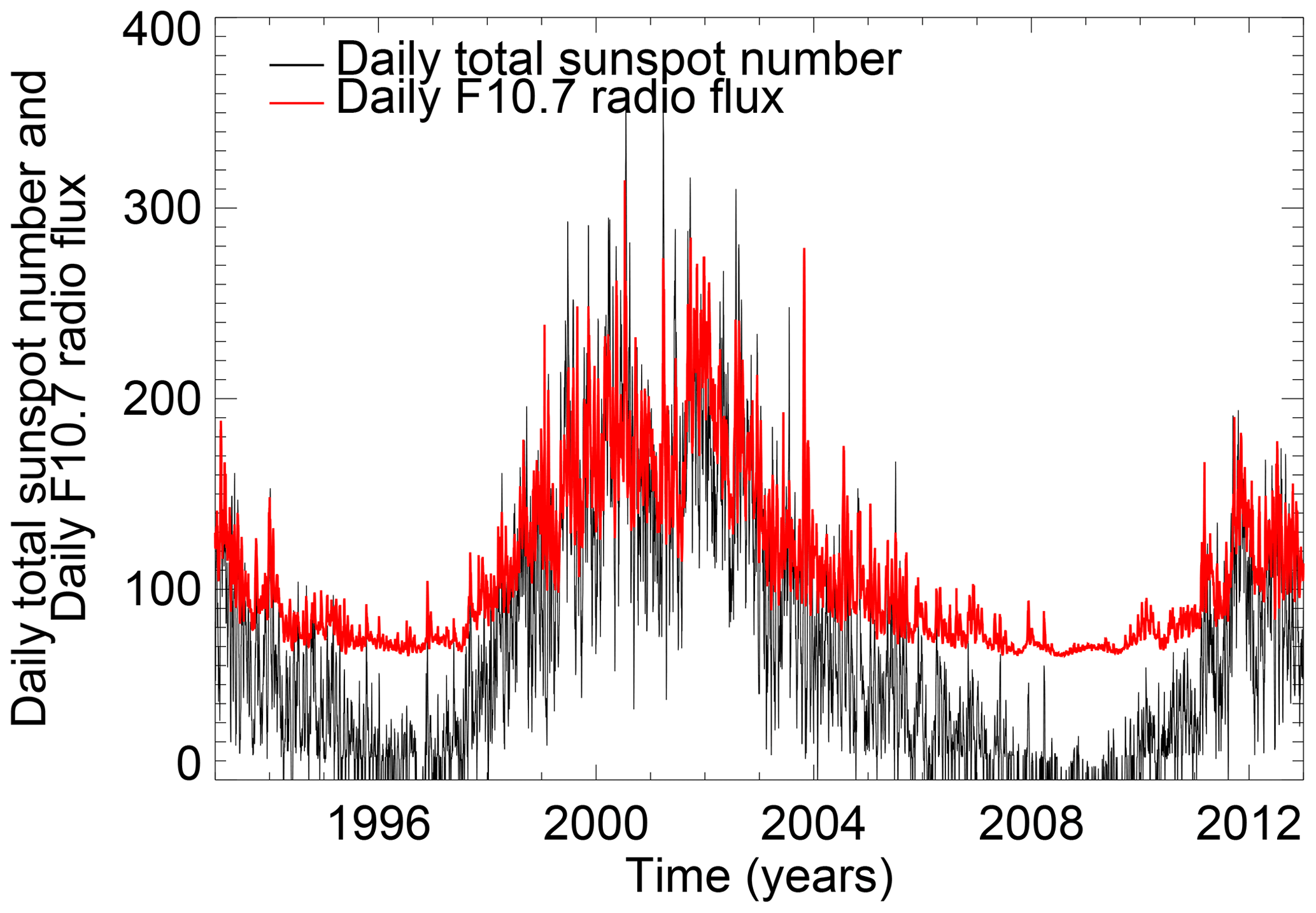
Figure 1 Daily sunspot number indicated in black and daily F10.7 radio flux indicated by the red line; adapted from David et al. (2018).

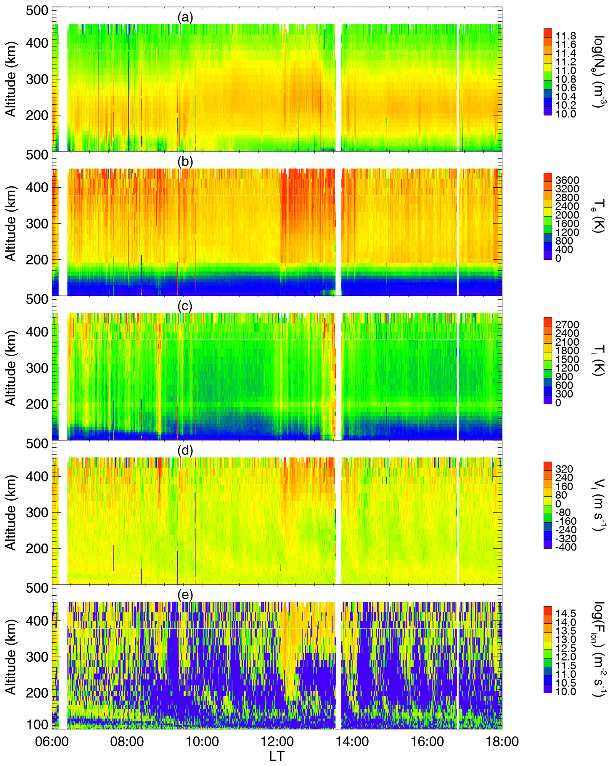
Figure 2 EISCAT Svalbard Radar (42 m dish) parameter plot for the dayside on 11 September 2007. The panels (a)–(e) are, respectively, the electron density, electron temperature, ion temperature, ion drift velocity and ion flux.

Table 1 shows the number of data points for both unfiltered and actual (filtered) data for each class of ion upflow flux as well as the percentages of the actual and noisy data. The actual data are the number of data points that satisfy the filtering technique (used in this work) set by David et al. (2018) for upwelling ions, while unfiltered data, on the other hand, are the number of data points before filtering that fell in the range of each class of upflow from the raw data obtained by the ESR during the period under investigation. The percentage of the actual data is calculated from the percentage ratio of the actual to the unfiltered data points. On the other hand, percentage noise for each class is obtained by

$$\mathrm{noise}=\left(\mathrm{1}-{\displaystyle \frac{\text{actual data point for each class}}{\text{unfiltered data point for each class}}}\right).$$

Table 1 Ion flux classification with associated signal and noise ratio.

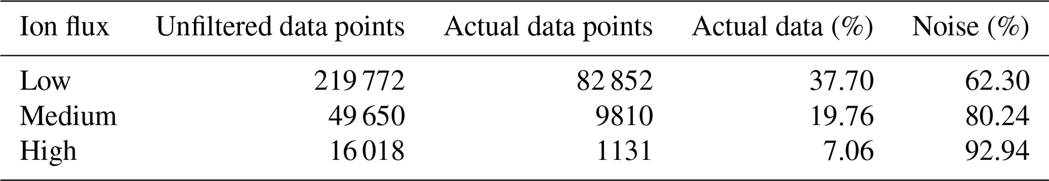
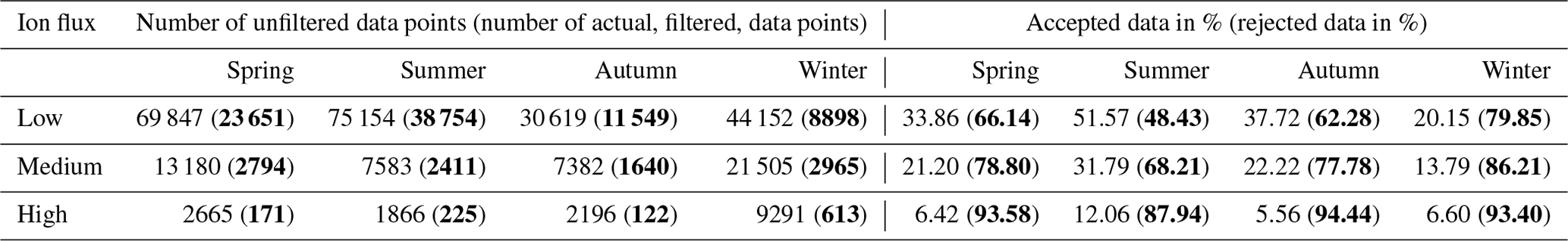
Table 2 Seasonal variation in the signal-to-noise ratio for different classes of ion flux upflow. The number of actual data points and the rejected data in % are in bold and in brackets.

The low-flux upflow is a common event and analysis of filtered data reveals that its frequency is about 8 and 73 times that of the medium- and high-flux upflow events, respectively. The data in Table 1 indicate that about 33 % of the ESR data satisfies the filter, of which about 29 % contribution is from the low-flux upflow, while medium- and high-flux upflow contribute about 3.4 % and 0.4 %, respectively. Investigation shows that the levels of noise in the three classes of upflow are about 62 %, 80 % and 93 % for the respective low-, medium-, and high-flux upflows. It is well known that ISR data are entangled in noise; the high-level occurrence observed here may be attributed to a low signal-to-noise ratio characterising much of the high-latitude data at a deep solar minimum around the period (David et al., 2018). It is therefore left open to research to investigate whether data outside the solar minimum would have a lower rejection rate.

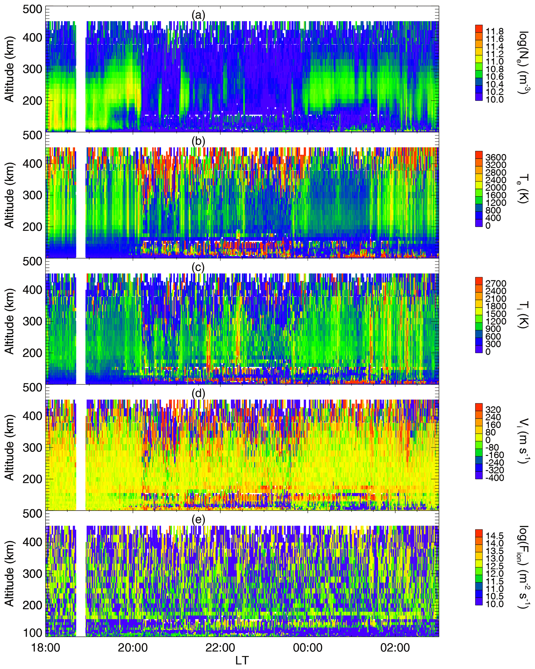
Figure 3 EISCAT Svalbard Radar (42 m dish) parameter plot for the nightside on 28 December 2007. The panels (a)–(e) are, respectively, the electron density, electron temperature, ion temperature, ion drift velocity and ion flux.

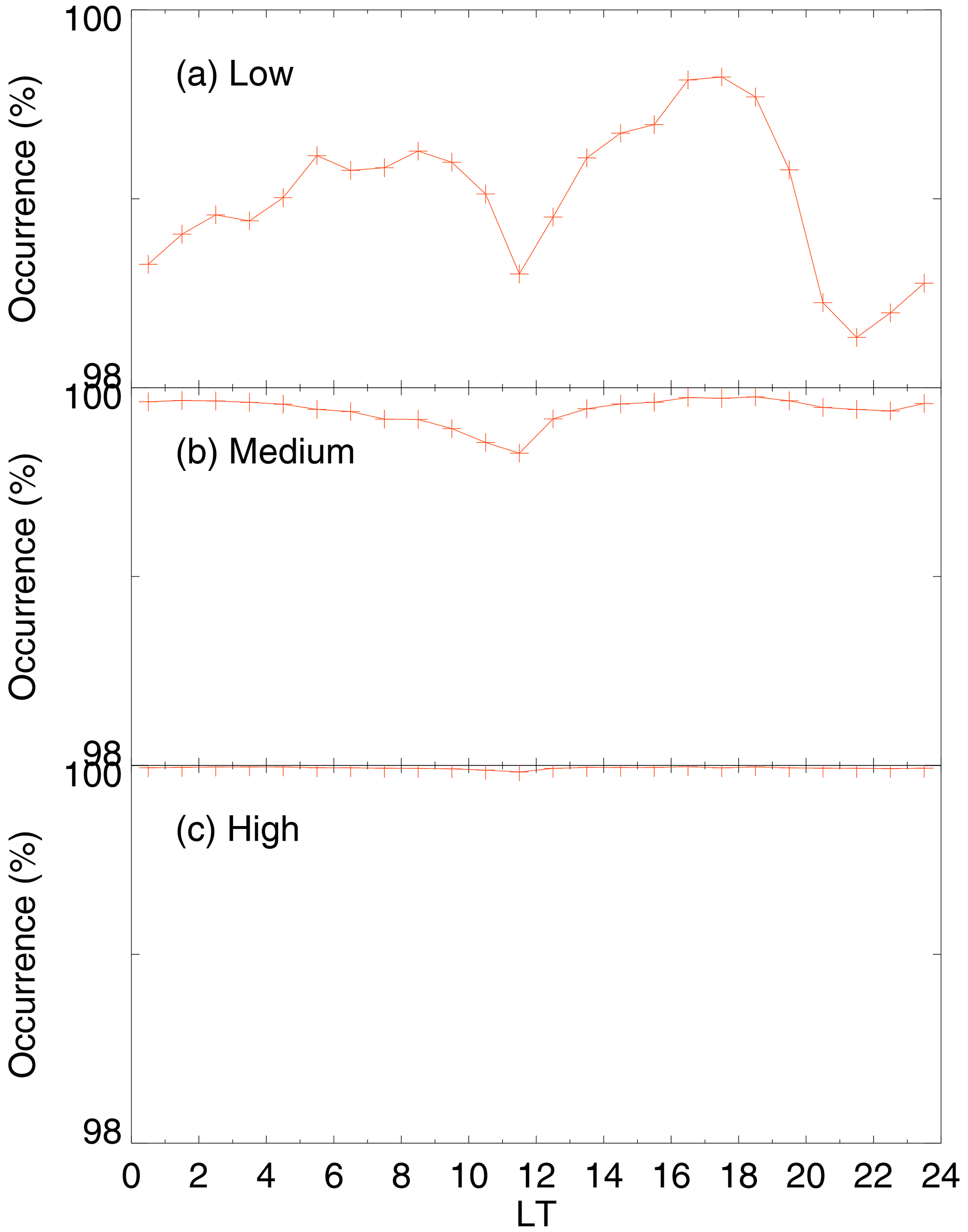
Figure 4 Local time distribution of noise occurrence in (a) low-, (b) medium-, and (c) high-flux upflow.

The geographical location of the ESR, reported by David et al. (2018), subjects it to variable radiation flux from the Sun and a variable rate of ionisation across the seasons. The result from Table 2, under the column for actual data/noise heading, reveals that the percentage of rejected data increases from low-flux upflow to high-flux upflow irrespectively of the season. The noise level in the low-flux upflow ranges from 48 %–80 % across the season, whereas the medium- and high-flux upflow, respectively, is 68 %–87 % and 87 %–95 %. However, there is no definite pattern across the season for the upflow classes. Moreover, the noise level for each category of upflow is predominantly high during winter and this is not unconnected with the radar data usually being of lower quality in winter. The noise, as expected, is minimal in summer, with a notable result as seen in the low flux showing the occurrence of actual data is about 51.6 % while noise is approximately 48.4 % – the only case in which actual data are above noise. Further analysis, as shown in Fig. 4, reveals the distribution of the three classes of ion flux upflows with respect to local time interval. Panel (a) in Fig. 4 shows the local time variation in the noise for the low-flux upflow, where a clear trough is observed around 12:00 LT and before midnight. The peak of the period when noisy data are observed is shown to be between 17:00 and 18:00 LT. The minimum percentage of the noise level across LT is above 98. Panel (b) in Fig. 4 also indicates that the noise level for the medium flux, though very high (above 99 % across LT), is the lowest around 12:00 LT. However, no distinct minimum is observed in the high-flux upflow shown in panel (c) in Fig. 4; in fact, the noisy data for the class approach 100 % for all local time.

It is worthy to note that the dip in the noise occurrence in Fig. 4 is a result of large ion outflows and an elevated ionisation rate, which are characteristics around the cusp (Welling et al., 2015). The contributory role to the suppression of noise in this sector as well as the midnight sector may be attributed, respectively, to the soft electron precipitation, which is characteristic of the abundant F-region ionisation, and the reconnection usually experienced on the nightside, leading to substorm.

In addition, it appears that the high level of rejected data is evident in ISR data, and, as a result, robust and stringent filtering techniques must be ensured when analysing incoherent radar data in order not to introduce bias to the result. Ogawa et al. (2009) and Endo et al. (2000) have pointed out that radar data are noisy in the topside ionosphere as a result of inadvertently obtained unphysical velocity, coupled with thermal noise from receivers, as well as uncertainties that arise from fitting line-of-sight velocity.

In light of the above, the proposed phased array ISR, named Sanya ISR, should take into cognizance an ISR that, in practice, will have a better SNR by ensuring the best radar system input constants, effectual scattering volume and spatial variability terms in space, as stated in the work of Li et al. (2020). The results of this work could also be integrated in the buildup of the EISCAT 3D to allow for comparison between the SNR of the Scandinavian Arctic infrastructure and the Sanya ISR, which is proposed to be the first multistatic ISR in a low-latitude region.

4 Summary and conclusions

Noise associated with incoherent scatter radar (ISR) data located at Longyearbyen in Svalbard has been investigated during the solar minimum and the results are summarised as follows:

• About 33 % of the raw data satisfies the filter, of which about 29 % contribution is from the low-flux upflow, while medium- and high-flux upflow contribute about 3.4 % and 0.4 %, respectively.

• Investigation shows that the levels of noise in the three classes of upflow are about 62 %, 80 % and 93 % for the respective low-, medium-, and high-flux upflows.

• The percentage occurrence of the noise level in the data increases with increasing flux strength, irrespective of the season.

• The noise level for each category of upflow is predominantly high during winter and minimal in summer.

• A notable result, as seen in the low-flux during summer, shows that the occurrence of actual data is about 51.6 %, while noise is approximately 48.4 % – the only case in which actual data exceeds noise.

• Local time variation indicates that the noise level peaked around 17:00–18:00 LT and hit a minimum around 12:00 LT.