On the relationship between the mesospheric sodium layer and the meteoric input function

This study examines the relationship between the concentration of atmospheric sodium and its meteoric input function (MIF). We use the measurements from the Colorado State University (CSU) and the Andes Lidar Observatory (ALO) lidar instruments with a new numerical model that includes sodium chemistry in the mesosphere and lower-thermosphere (MLT) region. The model is based on the continuity equation to treat all sodium-bearing species and runs at a high temporal resolution. The model simulation employs data assimilation to compare the MIF inferred from the meteor radiant distribution and the MIF derived from the new sodium chemistry model. The simulation captures the seasonal variability in the sodium number density compared with lidar observations over the CSU site. However, there were discrepancies for the ALO site, which is close to the South Atlantic Anomaly (SAA) region, indicating that it is challenging for the model to capture the observed sodium over the ALO. The CSU site had significantly more lidar observations (27 930 h) than the ALO site (1872 h). The simulation revealed that the uptake of the sodium species on meteoric smoke particles was a critical factor in determining the sodium concentration in the MLT, with the sodium removal rate by uptake found to be approximately 3 times that of the NaHCO₃ dimerization. Overall, the study's findings provide valuable information on the correlation between the MIF and the sodium concentration in the MLT region, contributing to a better understanding of the complex dynamics of this region. This knowledge can inform future research and guide the development of more accurate models to enhance our comprehension of the MLT region's behavior.

1 Introduction

Micro-meteoroids enter the Earth's atmosphere day and night, depositing their constituents into the atmosphere via ablation, creating a region that hosts various metal species, for example, Fe, K, Si, Mg, Ca and Na, in both their neutral and ionic forms (Plane et al., 2015, 2021, and references therein). The region is commonly referred to as the mesosphere and lower thermosphere (MLT), located between 75 and 110 km altitude. The metal layers in the MLT often serve as the tracers that facilitate the investigation of the dynamical and chemical processes within the region (Takahashi et al., 2014; Qiu et al., 2021). Quantitative measurements of metal atoms have been made since the 1950s (Hunten, 1967) via a variety of ground-based or spaceborne technologies (Koch et al., 2021, 2022). The large resonant scattering cross-section (Bowman et al., 1969) and the substantial presence of the sodium atom in the MLT make it one of the most researched metal layers in the atmosphere (Yu et al., 2022).

The sodium layer is usually studied via observations carried out by resonance lidars, satellites, and through Na D-line emission at 589.0 and 589.6 nm (Plane et al., 2012; Hedin and Gumbel, 2011; Langowski et al., 2017; Andrioli et al., 2020; J. Li et al., 2020). The sodium vertical profiles retrieved by lidars have been commonly used as a tracer to study atmospheric dynamics, such as gravity waves and wind shear. The long-term seasonal and short-term diurnal variabilities in metallic species have been investigated by several studies (Feng et al., 2013; Marsh et al., 2013; Cai et al., 2019a, b; Yu et al., 2022; She et al., 2023). A typical sodium chemistry scheme consists of neutral chemistry, ion chemistry and photolysis. The sodium chemistry research in recent years has primarily been based on the sodium chemistry model by Plane (2004), which has been cited in various subsequent works, including Bag et al. (2015) and references therein.

As meteoroids are the primary source of metal layers in the atmosphere, including the sodium layer, the meteoric input function (MIF) plays a crucial role in the modeling of metallic layers in the atmosphere. The MIF is a function designed to model the temporal and spatial variability in the meteoroid on the atmosphere (Pifko et al., 2013). Sporadic meteors are estimated to make up more than 95 % of the total meteoroid population, based on comparing the number of meteors originating from sporadic sources with those originating from known shower meteor sources (Chau and Galindo, 2008). This highlights the importance of incorporating sporadic meteor data in the MIF to accurately understand the sodium concentration in the mesosphere and lower-thermosphere (MLT) region as well as its correlation with meteoroid material input. It is well established that there are six apparent sources of sporadic meteors: North and South Apex (NA and SA, respectively), North and South Toroidal (NT and ST, respectively), and Helion and anti-Helion (H and AH, respectively) (Campbell-Brown, 2008; Kero et al., 2012; Li et al., 2022). However, the relative strength of these meteor radiant sources varies among the studies. For example, the NA and SA sources are found to be much stronger than other sources in results obtained with high-power large-aperture (HPLA) radars (Chau et al., 2007; Kero et al., 2012; Li and Zhou, 2019), while specular meteor radars found the difference to be much smaller (Campbell-Brown and Jones, 2006; Campbell-Brown, 2008). The detection sensitivity varies significantly among different facilities. For instance, the Arecibo Observatory (AO; 18° N, 66° W) detects approximately 20 times more meteors per unit area per unit time than the Jicamarca Radio Observatory (JRO; 12° S, 77° W) and at least 800 times more meteors than the Resolute Bay Incoherent Scatter North (RISR-N) radar (75° N, 95° W), despite all being HPLA facilities (Y. Li et al., 2020, 2023; Hedges et al., 2022). While meteor flux does exhibit variations based on time and latitude, these fluctuations alone cannot explain the magnitude of the observed difference.

Consequently, the total mass of the meteors that enter the Earth's atmosphere is subject to significant uncertainties. In the existing Whole Atmosphere Community Climate Model-Na (WACCM-Na) global sodium model (Dunker et al., 2015), the meteoric input function was modeled by placing a flux curve on each radiant meteor source with a definite ratio (more details can be found in Marsh et al., 2013). The flux curve model is based on observations carried out exclusively by the AO. Although the model can reproduce some of the flux characteristics of the meteors observed at the AO, it is a relatively simple model and, therefore, has several limitations (Li et al., 2022). One of the limitations is that the model cannot reproduce the velocity distribution of the meteors in radar observations.

This study introduces a new numerical model for sodium chemistry that utilizes the continuity equations for all Na-related reactions without steady-state approximations. The main objective is to investigate the relationship between the apparent sodium concentration and the MIF in the MLT region. We then compare the results of the new model with measurements from two instruments, namely, the Colorado State University (CSU) and the Andes Lidar Observatory (ALO) lidars. Furthermore, we compared the MIF derived from the new sodium chemistry model and lidar measurements from CSU and ALO against the results of the high-resolution meteor radiant distribution recently deduced from observations conducted at AO. Finally, we discuss the implications of these comparisons and suggest possible explanations for the discrepancy between the MIF derived from radar and those obtained from lidar observations.

2 The sodium chemistry model (NaChem)

2.1 Sodium chemistry

Numerical airglow models have been extensively used to investigate atmospheric airglow chemistry and gravity waves (Huang and Hickey, 2008; Huang and George, 2014; Huang, 2015). A new numerical sodium chemistry model, hereafter referred to as NaChem, was developed for this study. Table 1 lists the complete reactions and their corresponding rate coefficients used in NaChem, which includes neutral chemistry, ion chemistry and photochemistry. The dimerization reaction of NaHCO₃ (Reaction R25 in Table 1) is the outlet that removes Na atoms in the chemistry scheme. The Na atoms can also be removed by the uptake of sodium species onto meteoric smoke particles (Hunten et al., 1980; Kalashnikova et al., 2000; Plane, 2004), a process that can be turned on or off in the model. This study estimates the MIF in the numerical model by matching the amount of sodium atoms removed by the dimerization reaction and uptake, i.e., sodium sink, to maintain the observed sodium presence in the MLT. MIF is a function of time and latitude, representing the mass of meteoroid material entering Earth's atmosphere. Throughout the rest of the paper, the MIF estimated from the sodium chemistry numerical model will be referred to as MIF(s). On the other hand, the MIF derived from meteor radiant distribution will be referred to as MIF(m). The MIF(m) is determined through a 3-D meteoroid orbital simulation, a process similar to the seeding process discussed in Sect. 3.1 of Li et al. (2022), based on the meteor radiant distribution. MIF(m) is given in arbitrary units. Note that the meteor mass cannot be accurately determined via radar measurements; however, the seasonal variation in meteoroid material input can be represented by MIF(m). The estimation of meteor mass is further discussed in Sect. 5. In contrast, MIF(s) is expressed in units of 1 cm⁻³ s⁻¹.

The numerical model utilizes the continuity equation to track the time evolution of all 14 Na-related species. Table 2 presents a comprehensive list of these species, along with their corresponding production and loss rates. The background gas species, including species such as O₃, O₂, O, H, H₂ and H₂O, and the temperature are provided by WACCM version 6 (WACCM6; Jiao et al., 2022). Here, we use the dynamic version of WACCM nudged with version 2 of NASA's Modern-Era Retrospective analysis for Research and Applications (MERRA-2) reanalysis dataset (Hunziker and Wendt, 1974; Molod et al., 2015; Gettelman et al., 2019). The WACCM reference profiles are linearly interpolated to a resolution of 1 min and updated every minute during the simulation. It is worth noting that the Na-related reactions, which are illustrated in Table 2, do not significantly impact the background gas species, as the effect is orders of magnitude smaller than the variation in the major gas species themselves. Therefore, the major gas species are simulated independently of Na-related reactions.

2.2 Numerical scheme

As discussed earlier, it is worth noting that the reactions of sodium chemistry in NaChem share similarities with those in previous models (e.g., Plane et al., 2015, and references therein); however, the implementation of the numerical chemistry scheme differs. NaChem uses continuity equations to treat all chemicals involved, including short-lived intermediate species. Treating all species with the continuity equation is a straightforward and more accurate approach than using steady-state approximations. Moreover, by treating all species in a uniform manner, the numerical model is more compact and easier to interpret. The computational capability of a personal computer nowadays has advanced enough to process an ultrafine time step (microseconds) that is necessary for numerical simulations of short-lived species in a reasonable duration. Still, the differential equations for production and loss of short-lived species can be numerically unstable unless a microsecond or even sub-microsecond time step is used (Higham, 2002). The concern of the differential equation instability can be largely mitigated by a first-order exponential integrator (Hochbruck and Ostermann, 2010), i.e.,

$$\begin{array}{}\text{(1a)}& {\displaystyle }c=x_{\mathrm{0}}-{\displaystyle \frac{a_{\mathrm{0}}}{b_{\mathrm{0}}}},\text{(1b)}& {\displaystyle }{x}_{\mathrm{1}}={\displaystyle \frac{a_{\mathrm{0}}}{b_{\mathrm{0}}}}+c{e}^{-b_{\mathrm{0}}\mathrm{\Delta }t}.\end{array}$$

Here, x₀ is the value of the current step. In the simulation, it is the number density of the species. a₀ (1 cm⁻³ s⁻¹) is the production of the species, b₀ (1 s⁻¹) is the loss rate of the species, Δt is the step size in time and x₁ is the value of the next step. The units for x₀, x₁ and c are 1 cm⁻³.

The exponential integrator, as expressed in Eqs. (1a) and (1b), is the solution to the continuity equation. Note that Reaction (R25), listed in Table 1, is an exception that was carried out using an explicit Euler integrator in the simulation. This reaction's continuity equation is structured differently from the others because it represents the only mechanism for removing Na atoms from the chemistry simulation, apart from the uptakes of sodium species. Our testing indicates that both the exponential integrator and explicit Euler integrator yield nearly identical results. However, for numerical stability, the explicit Euler integrator requires a step size of ∼ 1 µs, which is orders of magnitude smaller than the exponential integrator. The default time step of NaChem is 0.1 s with the exponential integrator.

Table 1 Reactions in NaChem. f_a and f_x are branching ratios.

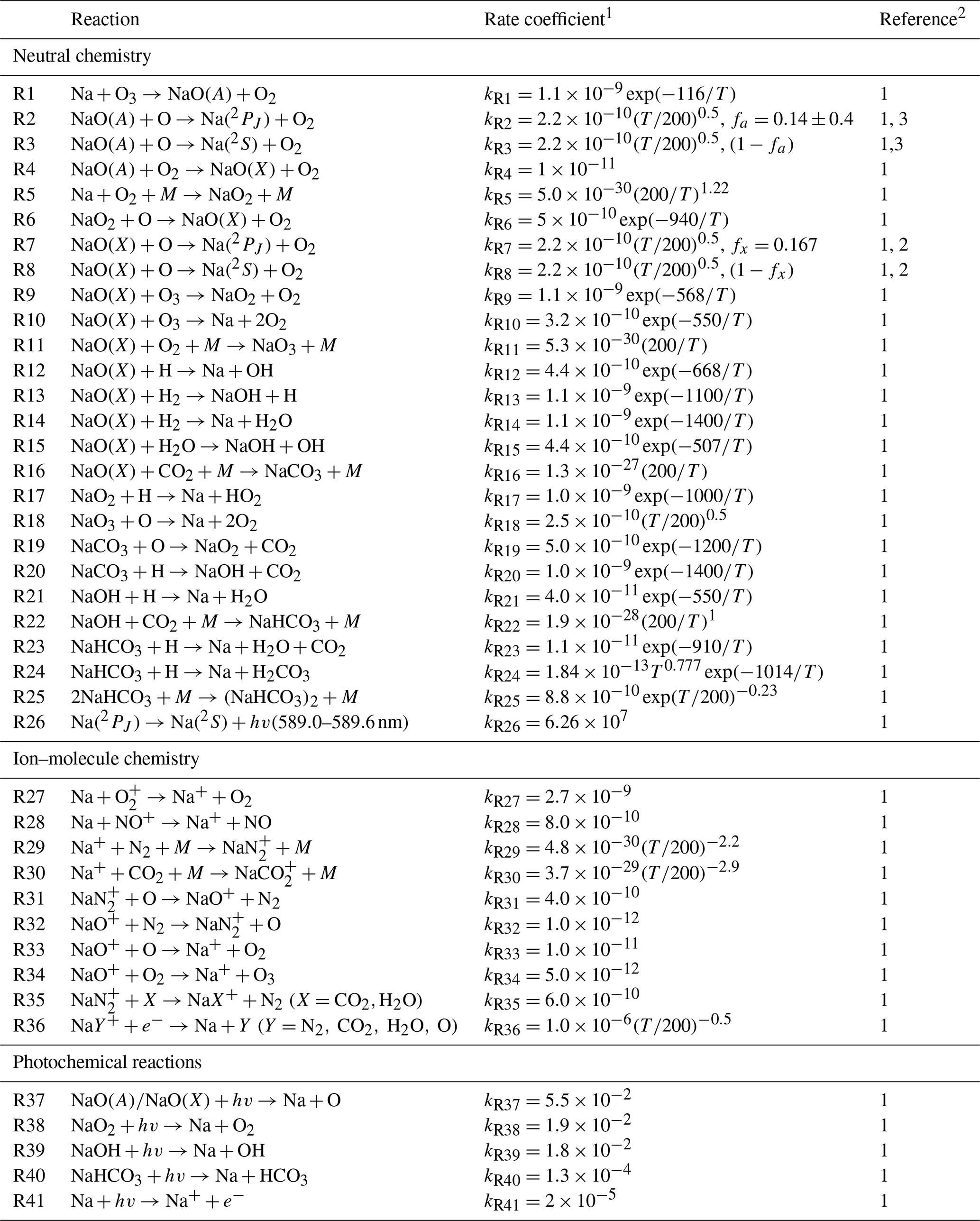
¹ Units for rate coefficient are as follows: unimolecular – per second (s⁻¹); bimolecular – cubic centimeters per second (cm³ s⁻¹); termolecular – sextic centimeters per second (cm⁶ s⁻¹); etc. ² The numerals in the “Reference” column refer to the following publications: 1 – Plane (2004); 2 – Plane et al. (2012); 3 – Griffin et al. (2001).

Table 2 The production and loss terms of the sodium-related species.

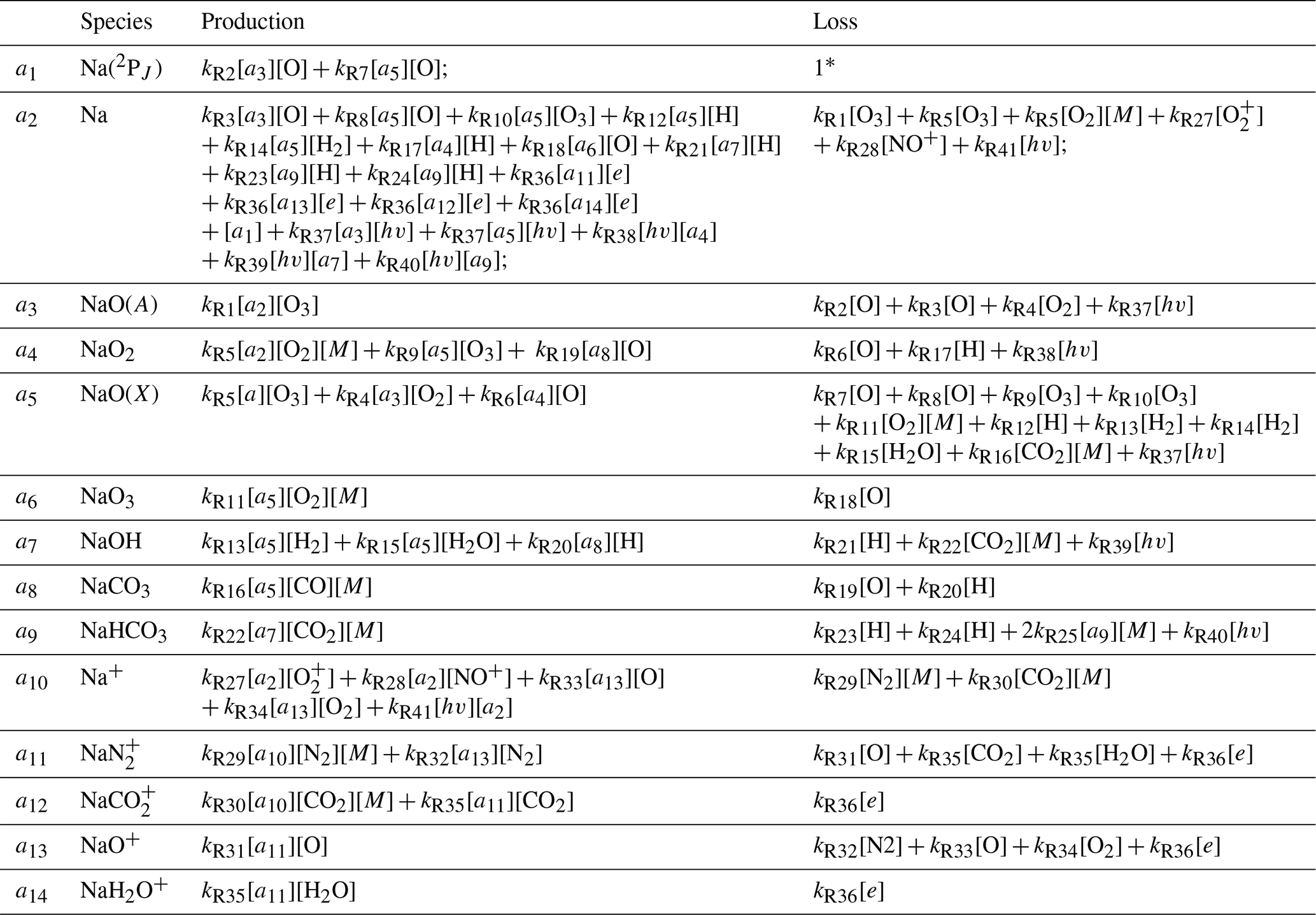
^* In Species 1, as of the current state of the model, all Na(²P_J) atoms return to their ground state immediately, so the loss term is set to 1. The [hv] is the term that represents loss via photoionization, which is approximately a sinusoidal function based on the solar zenith angle of the respective local solar time.

3 CSU and ALO sodium lidar observations and data processing

3.1 Observations

Several aspects of the current research, i.e., the presence of sodium in the MLT, require cross-validation with the measurements. One primary objective of the present model is to match the observed seasonal variation in the sodium layer. Measurements by the Colorado State University (CSU; 41.4° N, 111.5° W) lidar, also known as the Utah State University (USU) lidar, and the lidar data acquired by the Andes Lidar Observatory (ALO; 30.3° S, 70.7° W) are used to facilitate the research in the current study. We were unable to acquire more ALO data after 2019, as the COVID situation disrupted the site operation. The CSU data comprise 27 930 h of lidar observations between 1990 and 2020, whereas the ALO data consist of 1872 h between 2014 and 2019.

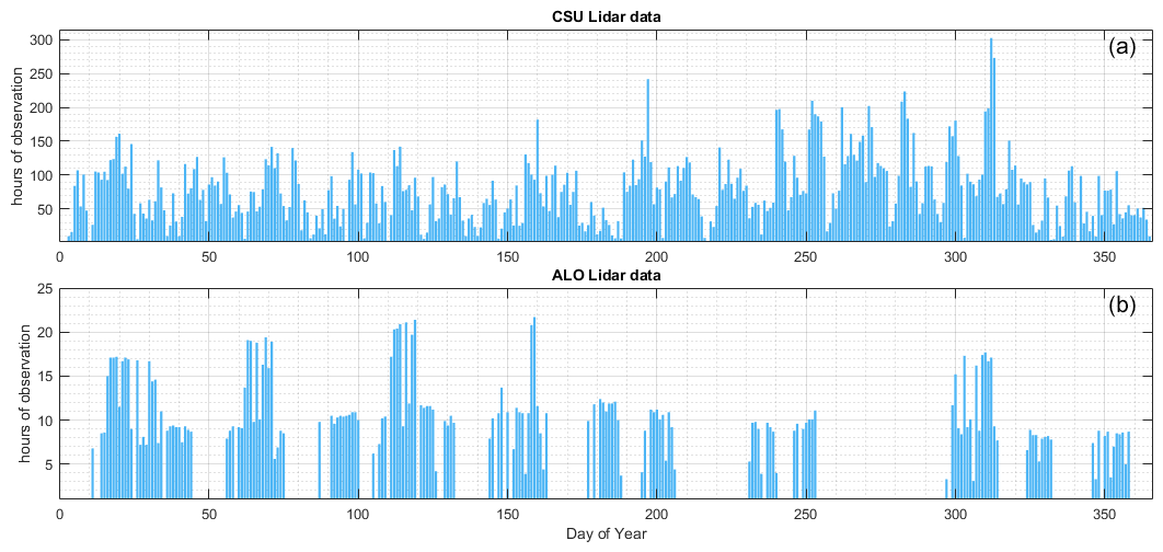
Figure 1 Available hours of lidar observations: (a) CSU lidar (1990–2020) and (b) ALO lidar (2014–2019).

The statistics of data available from CSU and ALO are presented in Fig. 1. The lidar observations from both sites consist of nocturnal observations only, and a typical nocturnal observation lasts between 8 and 11 h. Note that, in Fig. 1, there could be as many as 300 h of sodium observations on a single day of year, which means that the data of the date comprise observations from many different years on that day. The CSU data almost covered every day of the year with only a few exceptions, whereas the ALO data were much more sparse. As a result, due to the significantly larger number of CSU observations, the statistical reliability of the seasonal variation in the sodium layer derived from ALO observations may not be as strong as that of the CSU data. As depicted in Fig. 2, the overall seasonal trend in the sodium vertical profile derived from CSU lidar observations closely aligns with the simulation-based estimate by Marsh et al. (2013). In contrast, the ALO lidar observations deviate from the findings reported by Marsh et al. (2013). The ALO measurements exhibit a prominent peak around June, while the results in Marsh et al. (2013) show a double peak in March and October.

3.2 Data processing

The sodium layer in atmospheric observations is often affected by perturbations of atmospheric dynamics, which is why sodium is commonly used as a tracer in the study of the MLT dynamics (Plane et al., 2015). However, studying the sodium layer itself can be complicated due to the underlying chemical processes coupled with the dynamics. In order to mitigate the effects of atmospheric dynamics, we process the sodium vertical profiles from observations in three steps. First, we average the profiles by the day of the year, meaning that we take the average of the data from the same day of the year from different years. Missing data are treated using linear interpolation. Next, we smooth the averaged profiles using a 15 d running average. Finally, the height profile for each time step is further smoothed by fitting it with a skew-normal distribution (Azzalini and Valle, 1996), using the least-squares error method.

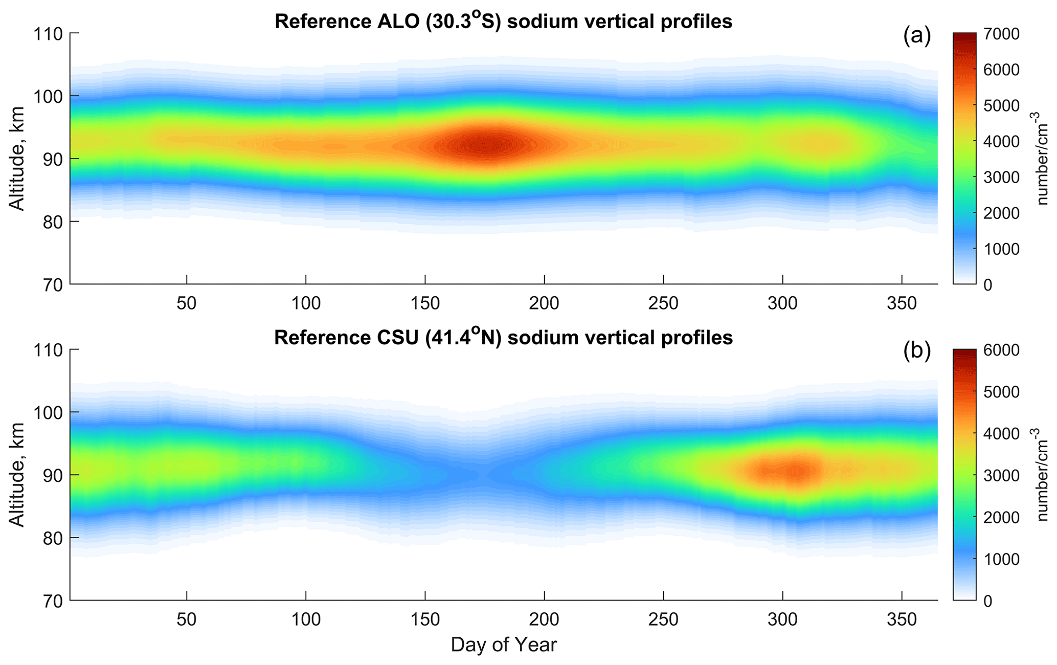
Figure 2 The reference annual sodium vertical profiles at the (a) ALO and (b) CSU. The reference profiles are the averages throughout all of the available data on the same days at the respective sites; these averages are fitted by a skew-normal distribution that mitigates atmospheric dynamics. In essence, the reference profiles are measurements with small-scale dynamics removed via the steps discussed in Sect. 3.2.

Figure 2 displays the processed annual sodium vertical profiles from the lidar measurements, referred to as reference profiles hereafter. These profiles serve as references to guide the numerical simulation of the NaChem model. The reference profiles are Na lidar measurements fitted using a skew-normal distribution, smoothed by a 15 d running average, and processed through linear 2-D interpolation across time and altitude. The lidar measurements have an altitude resolution of 500 m for the ALO and from 75 to 140 m for the CSU. These measurements are interpolated to a 100 m resolution as inputs to the NaChem model. The time resolutions of the lidar measurements typically vary between 1 and 10 min, depending on the experiment, and are linear interpolated to 0.1 s. The reference profiles inherently include diffusion and other dynamic effects on the sodium species in the MLT, as these observational data represent snapshots of sodium diffusion at various times. By constantly matching the observed Na profile to the simulated Na profile, the diffusion is included implicitly in the model. The seasonal column densities of both the ALO and CSU profiles are similar to a sinusoidal function, with the ALO data peaking near June and CSU data peaking in November. The centroid height of the sodium layer is higher in the ALO data than in the CSU data.

4 Results

4.1 Sensitivity test

Sodium in the atmosphere could manifest in many forms, i.e., in sodium-bearing neutral chemicals and ionic chemicals. The sodium number densities are typically obtained via lidar measurements. Given the complexity of the sodium chemistry, the observed sodium is merely a subset, possibly not even a major constituent, of the total number of all of the sodium-bearing species in the atmosphere. The total sodium content is defined as the total number of sodium atoms in all 14 sodium-bearing species, as listed in Table 2. In summary, the sodium that we can detect does not necessarily provide an accurate representation of the total sodium content or the overall count of sodium-bearing species, as unobservable species such as Na⁺ and NaHCO₃ could constitute a substantial portion of the total sodium content.

Understanding the impact of each background species, i.e., species listed in Fig. 3, on the total sodium content is essential to study the underlying mechanism of the chemical reactions. Therefore, we present a sensitivity test by isolating variables. The sensitivity test is done by altering the number density of background species in question by 2 orders of magnitude, i.e., by a factor of 0.1 and 10, while keeping the number densities of other background species and the atomic sodium fixed. The simulation is kept running until all of the numbers are stable. The diurnal variations in the sodium and background species are not considered in the sensitivity test, as they introduce unnecessary complexity. The results of the sensitivity test of the 11 background species and temperatures involved in the numerical simulation are shown in Fig. 3. Each panel contains three lines, where the red curve shows the unaltered vertical profile of the total sodium content. The results of the species altered by a factor of 0.1 and 10 are shown in light blue and yellow, respectively.

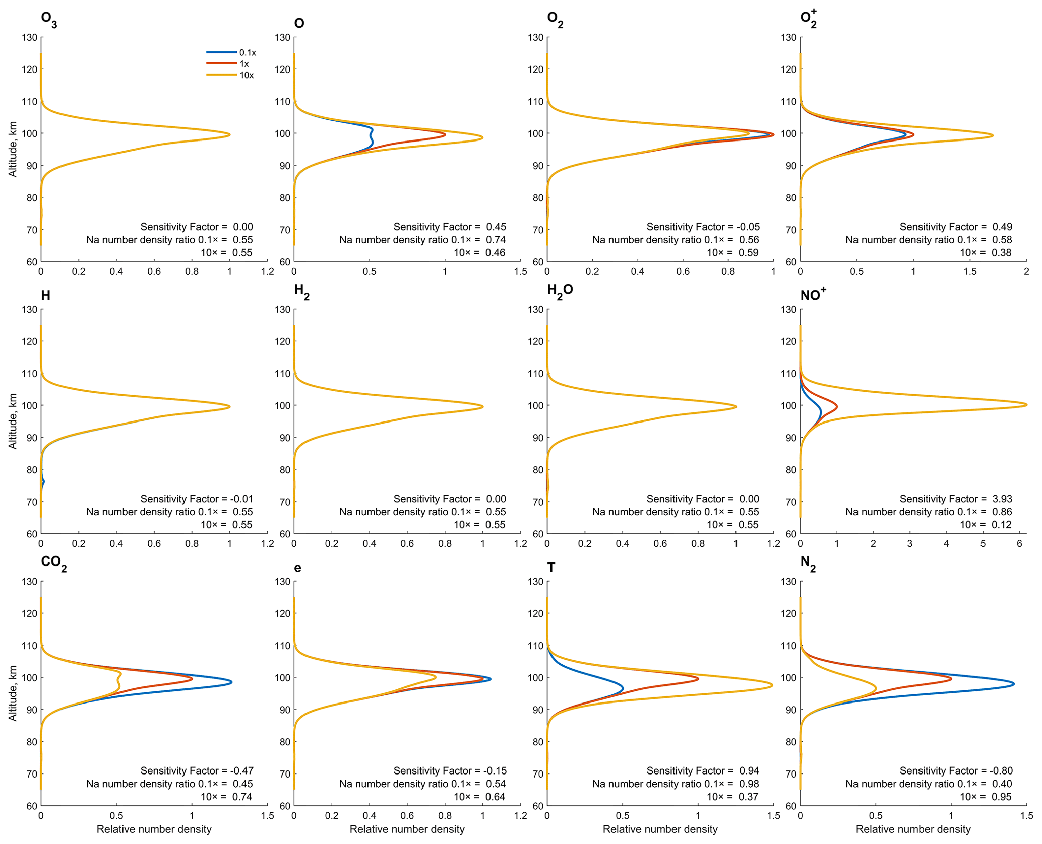
Figure 3 Sensitivity test of 11 background species and temperature on Na chemistry. The total sodium content vertical profile for the respective background species altered by a factor of 10 and 0.1 are shown in yellow and light blue, respectively. The reference sodium content vertical profiles are shown in red. Additionally, the sensitivity factor and the Na number density ratio to the concentration of all sodium species are presented in each panel.

In Fig. 3, only the yellow curve is visible in some of the panels because the three curves are drawn on top of each other, indicating that the change in the respective background species bears little to no effect on the sodium chemistry. A sensitivity factor is defined to better quantify the weight of each background species in sodium chemistry. The factor is calculated by the following equation:

$$\begin{array}{}\text{(2)}& \mathrm{sensitivity}\mathrm{factor}={\displaystyle \frac{{\mathrm{NaT}}_{\mathrm{c}}^{\mathrm{10}}-{\mathrm{NaT}}_{\mathrm{c}}^{\mathrm{0.1}}}{{\mathrm{NaT}}_{\mathrm{c}}}}.\end{array}$$

Here, ${\mathrm{NaT}}_{\mathrm{c}}^{\mathrm{10}}$ is the column density of the total sodium content with the respective species altered by a factor of 10; ${\mathrm{NaT}}_{\mathrm{c}}^{\mathrm{0.1}}$ is the same operation as the previous one but altered by a factor of 0.1. The denominator, NaT_c, is the column density of the reference profile. The sensitivity factor provides a general insight into how variations in the background species correlate with the sodium number density. A greater absolute value for the sensitivity factor indicates a stronger correlation. A positive sensitivity factor indicates a positive correlation between the total sodium content and the respective species, and vice versa. The reference profile is the total sodium content in steady state in the background condition of the midnight new year of 2002, giving a typical sodium vertical profile similar to the one shown in Fig. 5 of Plane (2004). In the simulation, a greater total sodium content implies that a smaller percentage of the sodium chemicals are present as sodium atoms, as the altitude profile of the sodium atoms is fixed in the sensitivity test. In reality, instead of the sodium atoms, the total sodium content should be more or less conserved. Hence, a higher total sodium content in our simulation suggests that less sodium can be detected by the lidar.

Although the sensitivity factor could be different upon a change in the reference profile, it still gives an insight into the significance of each background species with respect to the sodium chemistry. Apparently, the weight of some background species, namely, O₃, H, H₂ and H₂O, is negligible in sodium chemistry, meaning that removing these species and their associated reactions has no effect on the overall sodium chemistry. Nevertheless, these species are still kept in our numerical model for completeness. The impact of species that convert Na atom to Na⁺, as listed in Reactions (R27) and (R28) of Table 1, is generally strong. The effect of NO⁺, in particular, is the most significant according to the sensitivity factor, greater than the combined effect of all of the other species. Consequently, the number density of the observable [Na] atom by lidar is strongly anticorrelated with the fluctuations in the NO⁺. In a nutshell, more NO⁺ will directly lead to fewer observable Na atoms. That being said, the interaction between sodium and background species is rather complex. The scope of the sensitivity factor in the present paper was limited to column density. As a result, variations and behaviors of the sodium chemicals by altitude are overlooked. The actual impact of the background species may differ at different altitudes.

4.2 Meteoric input function

The estimation of meteoric influx is subject to many uncertainties among different techniques (Li et al., 2022). Moreover, the meteor flux estimated by the sodium chemistry model also varies (Marsh et al., 2013; Plane et al., 2015). The previous model of Plane (2004) and the following similar models indicate that the rate of dimerization, or the speed of removing sodium from the system, is heavily correlated with the vertical transport in the MLT. The NaChem model does not explicitly incorporate vertical transport, but the vertical transport by diffusion is inherently embedded within the input of the observed sodium vertical profile.

Unlike the previous models (Plane, 2004; March et al., 2013; and references therein), the present NaChem model took an indirect route to estimate the meteor mass input. During the simulation, the NaHCO₃ dimerization and the uptake of the sodium species on meteoric smoke particles, which can be turned on or off, create a deficit of sodium atoms. Meanwhile, a meteor input function injects an appropriate amount of sodium atoms so that the present sodium vertical profile always matches the reference profiles. This is carried out by finding the difference between the current sodium profile (with the deficit) and the corresponding reference profile in every iteration and then replacing the former with the latter. The study by Plane (2004) found that the diffusion coefficient is highly correlated with the sodium sink, primarily because the dimerization reaction occurs predominantly at lower altitudes. The simulation circumvents this uncertainty by directly incorporating the observational sodium vertical profile, given that diffusion is already inherently included in the measurements.

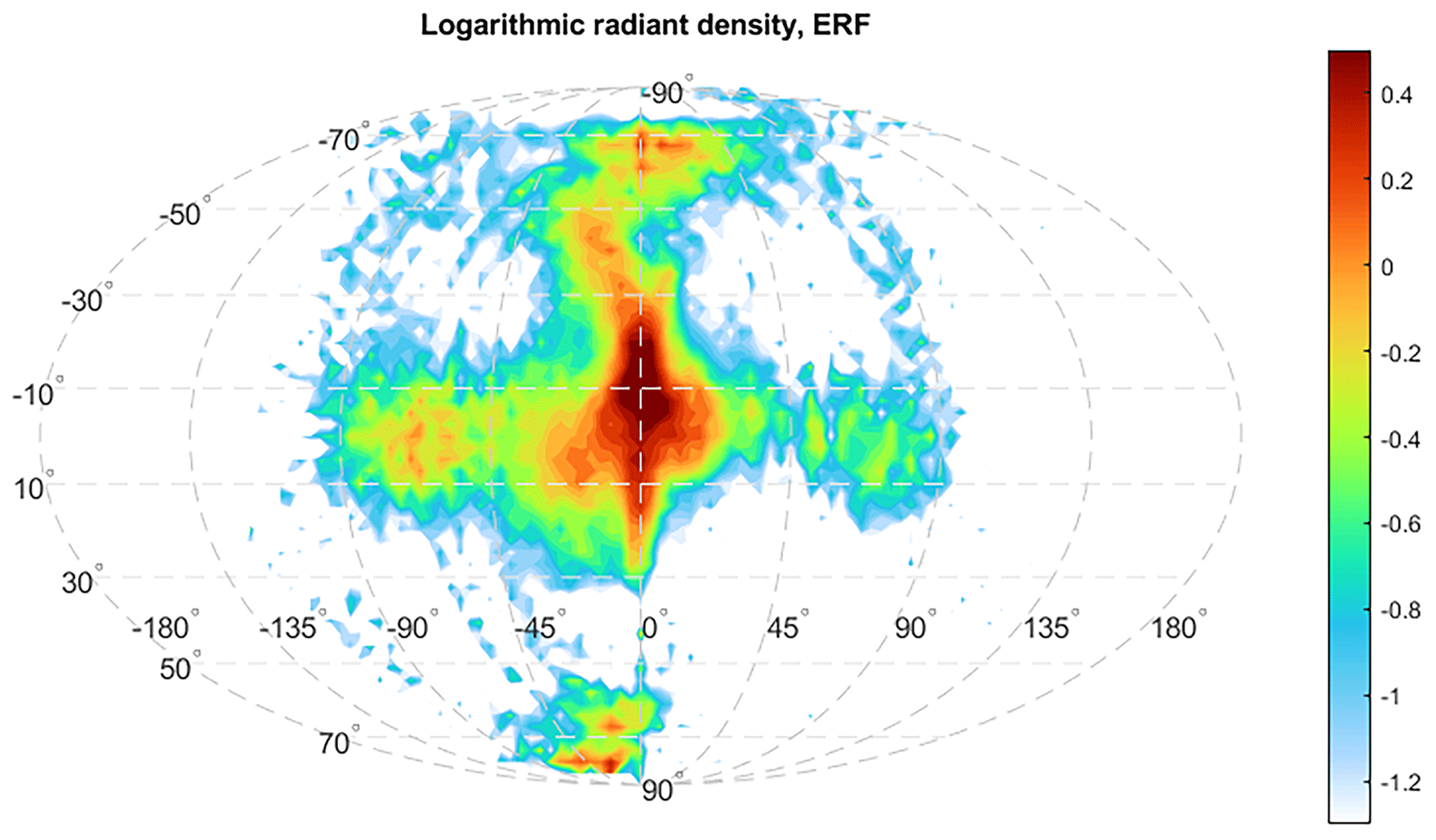
Figure 4 Logarithmic meteor radiant source distribution derived from the AO observations. The figure is in a.u. (arbitrary units). The figure illustrates the relative frequency of meteor occurrence at different radiant directions in the Earth reference frame (ERF), equivalent to ground-based observations. The latitude of the ERF is centered on the ecliptic plane. The longitude of the ERF is centered in the apex direction, the moving direction of the Earth, where the highest number of meteors encounter Earth. The radiant distribution is derived from the number of meteor events. The figure has been reproduced from Li et al. (2022).

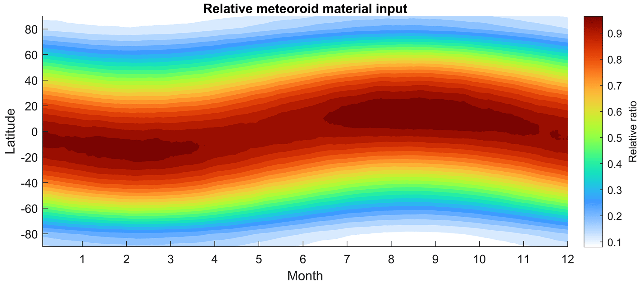
Figure 5 Relative seasonal and latitudinal meteoroid input by meteor occurrence, inferred from the radiant source distribution shown in Fig. 4. The figure is normalized to its max value.

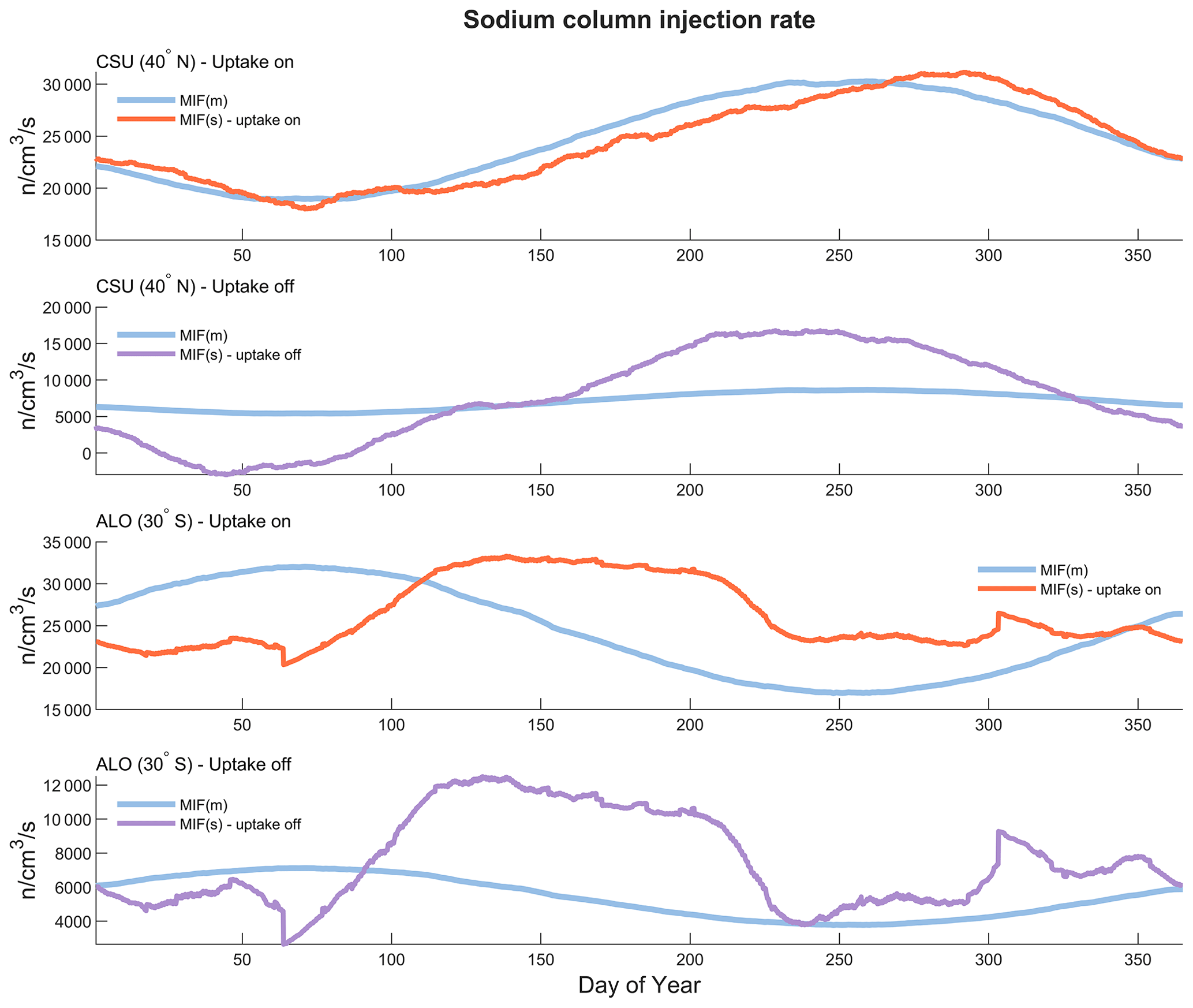
Figure 6 A comparison between two meteor input functions: MIF(m), which is inferred from the micro-meteor radiant distribution, and MIF(s), derived from an Na chemistry model with sodium input from lidar observations.

Figure 4 shows the high-resolution meteor radiant source distribution recently inferred from the AO observations (Li et al., 2022). The typical mass of the AO meteors is estimated to be around 10⁻¹³ kg based on the flux rate (Li and Zhou, 2019). Mathews et al. (2001) estimated the limiting meteor mass of 10⁻¹⁴ kg based on the meteor ballistic parameter. Limiting mass is the smallest mass a meteoroid must have to generate sufficient ionization to be detected by radar. Despite these estimations being based on various simplified assumptions that may lead to inaccurate results, the estimated limiting mass at AO is still at least 2 orders of magnitude smaller than the estimations of other facilities by similar means. More than 95 % of the meteoroid population in the Earth's atmosphere is found to be sporadic meteors by HPLA radar observation (Chau and Galindo, 2008), which are typically low-mass meteors evolved from the outer solar system due to the Poynting–Robertson drag (Nesvorný et al., 2011; Koschny et al., 2019). That being said, the percentage of sporadic meteors and the radiant source distribution are both estimated based on the occurrence. However, the occurrence of sporadic meteors may not be able to represent their mass distribution. The relative seasonal and latitudinal meteoroid input by the number of occurrence inferred from the new radiant source distribution is depicted in Fig. 5. The meteoric input generally follows a sinusoidal pattern and differs from the one used in the previous work, as shown in Fig. 1 of Marsh et al. (2013). Although the interplanetary dust (meteor) background on the Earth's orbit could vary in different locations due to a variety of reasons, e.g., Jupiter resonance, it is still safe to assume no change in the interplanetary dust background for our purpose. Taking a stable interplanetary dust background, the seasonal sinusoidal pattern of MIF(m) should follow the Earth's axis rotation relative to the ecliptic plane.

Figure 6 shows a comparison between two types of meteoric input functions: MIF(m), which is inferred from the micro-meteor radiant distribution, and MIF(s), derived using the Na chemistry model with sodium input from the lidar observations. MIF(m) is in arbitrary units and has been linearly scaled to match the amplitude of MIF(s). As for MIF(s), MIF(m) is also smoothed by a 15 d running average. For the MIF(s) model simulations, we used two scenarios, one with and one without uptake by smoke particles, for the ALO and CSU data. The MIF(s) with uptake by smoke particles exhibits a good match with the MIF(m) on the CSU dataset, while it does not show as good of a match on the ALO dataset. The MIF(s) with smoke uptake off is represented by a purple line, while the MIF(s) with smoke uptake turned on is depicted by an orange line. The MIF(s) could become negative when the reference sodium vertical profile decreases faster than the removal rate by the dimerization, as shown by the purple line in Fig. 6, indicating that the dimerization process alone is not sufficient to account for all of the sodium atom depletion in the MLT region. MIF(m) is derived from a global micro-meteor radiant distribution model, as depicted in Figs. 4 and 5. The smoke uptake of sodium species in this study is implemented using a methodology similar to Plane (2004); however, instead of applying smoke uptake solely to the three major sodium species, namely, Na, NaHCO₃ and Na⁺, it is applied to all 14 sodium-bearing species. The optimal uptake factor to obtain the best results was found to be $\mathrm{2}\times {\mathrm{10}}^{-\mathrm{2}}$ km⁻¹ s⁻¹. The smoke uptake and NaHCO₃ dimerization account for approximately 75 % and 25 % of the Na sink, respectively.

According to the global meteoroid orbital model outlined in Li et al. (2022), the latitudes spanning 29.5 to 30.5° S (ALO) account for 0.52 % of the total meteor input, while those between 39.5 and 40.5° N (CSU) represent 0.67%. The CSU site shares more meteor input due to its closer proximity to one of the apex meteor radiant sources. The global total sodium injection rate inferred from the ALO-data-based simulation is (2.01±0.68) × 10²³ atoms s⁻¹, while the CSU-data-based simulation suggests a global sodium injection rate of (1.28±0.55) × 10²³ atoms s⁻¹. The error is determined by calculating the standard deviation of the detrended, unsmoothed raw MIF(s). Note that both MIF(m) and MIF(s), presented in Fig. 6, are smoothed by a 15 d running average. Assuming that the relative sodium elemental abundance in meteoroid material is 0.8 % (Vondrak et al., 2008), the deduced total meteoroid material input of the ALO-based simulation is 83±28 t d⁻¹. From CSU-based simulation, the rate is 53±23 t d⁻¹. Both estimations are close to 80–130 t d⁻¹, the value reported by the Long Duration Exposure Facility (Love and Brownlee, 1993; McBride et al., 1999). It is worth noting that the estimated total daily input of meteoroid materials varies among previous studies, ranging from 4.6 t d⁻¹ (Marsh et al., 2013) to 300 t d⁻¹ (Nesvorný et al., 2010), with an intermediate value of 20 t d⁻¹ reported by Carrillo-Sánchez et al. (2020). While these estimates seem quite disparate, the variance is relatively small given that the daily input rate is derived from combinations of chemicals that can fluctuate by several orders of magnitude. For example, the NO⁺, which exhibits the highest sensitivity factor according to the sensitivity test, undergoes diurnal variations in approximately 3 orders of magnitude.

5 Discussion

The sodium concentration in the sodium layer in the MLT region is governed by several factors, including chemistry, dynamics and the MIF. It is difficult to discern which of these three components is more important than the others. In this section, we discuss various factors that may contribute to modeling the sodium concentration in the MLT.

The mass of the meteoroids has been estimated and measured using various methods. These include the ballistic parameter derived from meteor deceleration (Mathews et al., 2001), estimation of meteor head echo plasma distribution through a combination of meteor ablation models and radar cross-section measurements (Close et al., 2005; Sugar et al., 2021), flux rate determination (Zhou and Kelley, 1997), and spacecraft in situ measurements (Leinert and Grün, 1990), among others. The mass estimated by the meteor ballistic parameter is commonly referred to as momentum or dynamical mass. The mass estimated by the meteor ablation model is usually called the scattering mass. The meteor momentum mass from AO ultrahigh-frequency (UHF) radar observation is estimated to be 10⁻¹⁴–10⁻⁷ kg, with the typical mass being 10⁻¹³ kg. On the other hand, the meteor scattering mass is estimated to be 10⁻⁹–10^−5.5 kg by data from the EISCAT (European Incoherent Scatter Scientific Association) UHF radar (Kero et al., 2008) and 10⁻⁷–10^−4.5 kg by data from the ALTAIR (ARPA Long-Range Tracking And Instrumentation Radar) UHF radar (Close et al., 2005). While the detection sensitivity among different facilities differs, these estimations are still off by many orders of magnitude. The assessments of either momentum mass or scattering mass are based on a variety of simplified assumptions. They are subject to errors due to the complexity of radar beam patterns, background atmosphere conditions, aspect sensitivity, meteor radiant sources and many other possible factors. For example, meteor radar observation is subject to bias against low-mass, low-velocity meteors (Close et al., 2007; Janches et al., 2015).

Another aspect that may contribute to MIF(m) uncertainty is the meteor radiant distribution. The meteor radiant distributions, shown in Fig. 4 and many other studies (Chau et al., 2007; Campbell-Brown and Jones, 2006; Kero et al., 2012), are inferred or measured by meteor occurrence instead of mass input. Currently, retrieving a more accurate estimation of the meteor mass input is still a topic under active research, and there is no quantitative study on the disparities between meteor occurrence and meteor mass input. The radiant sources of the meteors are expected to differ by mass, as their orbital evolution is highly correlated to their mass. The interplanetary dust interacts with the solar wind while in the solar system, losing its momentum in the process and evolving into orbits with a smaller semi-major axis and lower eccentricity. The effect is called the Poynting–Robertson effect (Robertson, 1937), which behaves like a drag force and defines the evolution of interplanetary dust, and it could be the major reason for the existence of sporadic meteors (Li and Zhou, 2019; Koschny et al., 2019). The importance of the Poynting–Robertson effect is highly dependent on the density and mass of the object. By and large, the orbits of the smaller particles evolve exponentially faster. The orbital dynamics of interplanetary particles have been very well summarized in Sect. 2.2 of Koschny et al. (2019). For the reasons above, the meteor radiant distribution of mass could deviate from the radiant distribution of occurrence. Therefore, the meteor input rates, as shown in the blue curves of Fig. 6, could be different from those derived from the meteor radiant distribution of mass because they were derived from the meteor radiant distribution by occurrence.

In the sodium chemistry model presented in this work, the MIF is the sole source of sodium, while the sodium sink comprises NaHCO₃ dimerization and smoke uptake. The MIF(s) is determined by matching the sink rate of the sodium atoms with the rate of sodium injection. In other words, MIF(s) represents the amount of sodium injection needed to keep the sodium concentration equal to the reference sodium profiles. If the chemical lifetime of sodium in the MLT is short, then the seasonal variation in both the MIF and sodium concentration in the MLT should be similar. After examining Figs. 2, 5 and 6, it can be observed that the averaged seasonal variation in sodium over the years at both sites (ALO and CSU) does not correspond to the trend in the MIF(m) at their respective latitudes. This may indicate that the chemical lifetime of sodium in the MLT should be relatively long, as there is no immediate effect of MIF(m) on the sodium concentration. The MIF(m) displays a sinusoidal pattern that peaks in March at the ALO's latitude and in August at the CSU's latitude, whereas the sodium layer shows dual peaks in the CSU lidar observations and one peak in June in the ALO lidar observations.

In this study, the MIF(s) derived from the NaChem simulation, based on the CSU lidar measurements with uptake turned on, was able to match the amplitude of MIF(m) obtained from the meteor radiant distribution. Although the model does not directly incorporate any dynamical processes, the vertical transport by diffusion is implicitly included. The model forces the sodium layer to be the same as the data, which are derived from the average of many years' measurements, in which the diffusions are inherently embedded. The combination of observational data with the numerical chemistry model in this paper is a relatively straightforward application of data assimilation (Bouttier and Courtier, 2002). The lidar data of both sites (CSU and ALO) indicate that the sodium column density consistently increases by about 20 % from 22:00 to 04:00 LT the next day. This can be attributed to the fact that, during nighttime, the large deposits of Na⁺ formed by daytime reactions are slowly neutralized to Na. As a result, the sodium column density consistently increases throughout the night. The same effect can be reproduced in the NaChem simulation, albeit with a smaller amplitude. The simulation shows the increase to be about 8 %. The value is obtained by maintaining a constant total number of sodium-bearing species through the deactivation of the sodium sink.

While meridional transport or atmospheric dynamics both contribute to the seasonal variation in the sodium layer in the MLT, the diurnal sodium profile is the mean of observations of thousands of days, of which the variation by atmospheric dynamics should be much less prominent. The lack of explicit dynamics in the model may be one of the sources of inconsistency when compared to the MIF(m) observations. Further, WACCM6, which supplied the background species to NaChem, is an older version that does not fully incorporate the dynamics of each ion species. Despite our results showing good agreement between the MIF(s) and MIF(m), there might be several plausible factors that could lead to potential errors. For example, the Na sink by NaHCO₃ dimerization varies by the diffusion rate or the vertical transport of sodium atoms in the chemistry model (Plane, 2004). Likewise, the MIF(m) may also differ if the meteoroid mass input differs from the radiant source distribution by the occurrence of meteors, as discussed in the aforementioned paragraph.

6 Conclusion

This work introduced a new sodium chemistry model that simulates the time evolution of all sodium-bearing species using the continuity equation without making any steady-state assumption. The model employs an exponential integrator and runs with a high time resolution to maintain numerical stability. The model is simple to maintain in such a configuration and can be scaled up to include additional capabilities more easily. The model is highly optimized for processing efficiency and benefits from the use of an exponential integrator. Therefore, within an acceptable total CPU time, NaChem can afford a temporal resolution of up to milliseconds, several orders of magnitude smaller than those used in other Na models. During our testing, the ratio of CPU time to simulated real time is about 1 to 1000 using a 0.1 s time step.

The model simulation was able to reproduce the seasonal variation in the sodium layer in the MLT by simulations of chemical reactions. The simulation results at the CSU's latitude capture the general trend in the seasonal variation at the location. The MIF(s) based on the ALO data exhibited less conformity with the corresponding MIF(m), which could be attributed to inadequate statistics of the observational data. Comparably, the CSU dataset is more reliable, as the insufficient lidar hours in the ALO dataset may lead to inaccurate statistics. In the simulation, when forcing the sodium layer to be the observation-based reference profile, the inferred MIF is estimated to be 83±28 t d⁻¹ at the ALO and 53±23 t d⁻¹ at CSU. The numerical simulation by NaChem could reproduce the general trend in the diurnal and seasonal variation in the sodium layer compared to the observations by the CSU lidar. There are some inconsistencies in MIF(m) and MIF(s) based on data obtained from the ALO lidar. These inconsistencies may have originated from poor statistics resulting from insufficient observation hours.

In summary, a new sodium chemistry model has been developed in this work to investigate the relationship between the MIF and the sodium layer. We also compared the MIF(m) derived from radar meteor observation to the MIF(s) derived from the chemistry model and lidar observations. Our results indicate that the uptake of sodium species onto meteoric smoke particles removes approximately 3 times more sodium than the dimerization of NaHCO₃. Our future work will focus on incorporating the plausible factors that may lead to potential errors discussed above into the chemistry model.