the Creative Commons Attribution 4.0 License.
the Creative Commons Attribution 4.0 License.
 | 13 Jun 2024
Scale size estimation and flow pattern recognition around a magnetosheath jet
Adrian Pöppelwerth
Georg Glebe
Johannes Z. D. Mieth
Florian Koller
Tomas Karlsson
Zoltán Vörös
Ferdinand Plaschke
Transient enhancements in the dynamic pressure, so-called magnetosheath jets or simply jets, are abundantly found in the magnetosheath. They travel from the bow shock through the magnetosheath towards the magnetopause. On their way through the magnetosheath, jets disturb the ambient plasma. Multiple studies already investigated their scale size perpendicular to their propagation direction, and almost exclusively in a statistical manner. In this paper, we use multi-point measurements from the Time History of Events and Macroscale Interactions during Substorms (THEMIS) mission to study the passage of a single jet. The method described here allows us to estimate the spatial distribution of the dynamic pressure within the jet. Furthermore, the size perpendicular to the propagation direction can be estimated for different cross sections.
In the jet event investigated here, both the dynamic pressure and the perpendicular size increase along the propagation axis from the front part towards the center of the jet and decrease again towards the rear part, but neither monotonically nor symmetrically. We obtain a maximum diameter in the perpendicular direction of about 1 RE and a dynamic pressure of about 6 nPa at the jet center.
- Article
(2727 KB) - Full-text XML
- BibTeX
- EndNote


The magnetic field of Earth is an obstacle to supersonic solar wind. To flow around the magnetopause, the boundary between the terrestrial and interplanetary magnetic fields (IMFs), the solar wind must be decelerated to sub-magnetosonic speeds. This takes place upstream at the bow shock where the solar wind is decelerated, heated and deflected.
Depending on the angle θBn between the bow shock normal and the IMF, the bow shock can be divided into a quasi-parallel (θBn<45°) or quasi-perpendicular (θBn>45°) shock (e.g., Balogh et al., 2005). Particles reflected at the quasi-parallel shock can travel far upstream along the IMF and interact with the incoming solar wind. This leads to a region called foreshock which hosts a zoo of instabilities and waves (Eastwood et al., 2005). The waves are convected back to the shock with the solar wind, causing a rippled and undulated quasi-parallel bow shock.
The region between the bow shock and the magnetopause is called the magnetosheath (e.g., Spreiter et al., 1966). In the magnetosheath, localized enhancements in the dynamic pressure are frequently observed. These so-called magnetosheath jets (see the review by Plaschke et al., 2018) were first reported by Němeček et al. (1998). Various definitions of jets can be found in the literature, which compare the dynamic pressure enhancement, e.g., with the ambient plasma (e.g., Archer et al., 2012) or with the upstream solar wind (e.g., Plaschke et al., 2013). Jets are observed more often behind the quasi-parallel bow shock (e.g., Vuorinen et al., 2019), which corresponds to low IMF cone angle conditions for the subsolar magnetosheath, and favor quiet solar wind (e.g., Plaschke et al., 2013). LaMoury et al. (2021) and Koller et al. (2023) further investigated the statistical dependence of jet occurrence on solar wind parameters. Jet impact rates determined by LaMoury et al. (2021) showed that more magnetosheath jets impact the magnetopause under low IMF magnitude, low solar wind density and high Mach number conditions. However, the dominant occurrence-controlling parameters are low IMF cone angles and high solar wind speeds.
Jet formation downstream of the quasi-parallel bow shock may be explained by a mechanism suggested by Hietala et al. (2009, 2012). At the undulated bow shock, the incoming solar wind will be less decelerated and heated when passing the inclined parts. The geometry of the ripples can cause the flow to converge or diverge, resulting in density increases or decreases behind the shock. This leads to plasma regions with higher velocity and density than in the surrounding magnetosheath. Jets may also form due to solar wind discontinuities interacting with the bow shock (e.g., Archer et al., 2012). For example, hot flow anomalies (HFAs, e.g., Savin et al., 2012) or short large-amplitude magnetic structures (SLAMS, e.g., Schwartz and Burgess, 1991) can cause additional shock rippling when passing through the shock (e.g., Karlsson et al., 2018; Raptis et al., 2022b). This was also visible in simulations by Suni et al. (2021). They showed that jets can form due to the impact of compressional structures (like SLAMS) at the bow shock.
Geoeffective jets (with diameters > 2 RE) reach the magnetopause several times per hour (Plaschke et al., 2020a) and therefore have a big impact on the magnetosphere and ionosphere. They can indent the magnetopause (e.g., Shue et al., 2009), can cause surface waves (e.g., Archer et al., 2019), and may even penetrate through the boundary (e.g., Dmitriev and Suvorova, 2015). In addition, Němeček et al. (2023) showed in a statistical study that jets can be an explanation for extreme magnetopause positions and deviations from the model predictions. Hietala et al. (2018) showed that jets can trigger and suppress reconnection at the magnetopause, as they can modify the magnetic field in the magnetosheath and thus alter the shear angle at the magnetopause. This leads to situations where reconnection is triggered when it is not expected and vice versa (see also Vuorinen et al., 2021). Additionally, upon impact, jets can enhance ionospheric flow channels (Hietala et al., 2012) and disturb radio communication (Dmitriev and Suvorova, 2023). Nykyri et al. (2019) proposed that jets might even trigger substorms, leading to auroral brightenings. Also, Han et al. (2017) hypothesized in a statistical study that jets impacting the magnetopause might be one possible source of throat auroras.
On their way from the bow shock to the magnetopause, plasma jets interact with the ambient magnetosheath plasma. Palmroth et al. (2021) used global hybrid-Vlasov simulations to study the evolution of jets inside the magnetosheath. They reported that the jets thermalize on their way to the magnetopause and become more “magnetosheath-like” while they keep their propagation direction. In addition, Raptis et al. (2022a) reported that jets may contain two plasma populations, a cold and fast jet and a hotter and slower background population. Not only the jets but also the ambient plasma are affected by the interaction. Recent studies showed a slight alignment of the magnetic field in the jet propagation direction (Plaschke et al., 2020b) and a stirring of the magnetosheath plasma in the vicinity of the jet (Plaschke et al., 2017). Plaschke and Hietala (2018) reported in a statistical analysis that jets push slower plasma ahead of them and out of their way. Jets act like plows, and after their passage, the magnetosheath plasma fills the wake regions behind them. Plaschke and Hietala (2018) speculated that properties of jets like their scale size may influence the interaction.
Multiple studies report that magnetosheath jets have scale sizes on the order of 1 RE in the directions parallel and perpendicular to the jet propagation. To obtain a simple estimation of the parallel size of a jet, it is sufficient to integrate the plasma velocity over the jet observation interval (Plaschke et al., 2020a) or multiply the duration of the jet interval by the maximum speed to get an upper size limit (Gunell et al., 2014). To obtain the perpendicular size, at least two spacecraft are needed. Plaschke et al. (2016, 2020a) and Gunell et al. (2014) used pairs of spacecraft and derived the scale sizes in statistical studies from the probabilities of both spacecraft observing a jet. Karlsson et al. (2012) used the four Cluster spacecraft (Escoubet et al., 2001) to investigate the scale sizes of single jets. The authors performed a minimum variance analysis to obtain a suitable, jet-specific coordinate system. They extrapolated density profiles in these directions with linear fits allowing them to estimate the scale sizes in all three directions.
However, apart from Karlsson et al. (2012), all the aforementioned authors used statistical analyses to obtain information on the scale sizes and other properties of magnetosheath jets. Here we show for the first time the spatial distribution of the dynamic pressure within different cross sections of a jet. To achieve this, we select a jet event observed by the Time History of Events and Macroscale Interactions during Substorms (THEMIS) spacecraft (Angelopoulos, 2008) and transform the velocity measurements into a coordinate system aligned with the jet propagation direction. We use the vortical behavior of the plasma in the jet path (Plaschke and Hietala, 2018) to determine the position of the spacecraft within the plane perpendicular to the propagation direction. Ultimately, we use the positions and measurements of the spacecraft to estimate dynamic pressure profiles perpendicular to the propagation direction within different cross sections. In addition, we determine the perpendicular sizes with these profiles for different cross sections.
We focus on a jet observed by the THEMIS A, D and E spacecraft (THA, THD and THE) on 13 October 2010, around 16:04:00 UT. Measurements of the magnetic field (FGM, Auster et al., 2008), ion velocity, ion density, ion energy flux density and dynamic pressure (ESA, McFadden et al., 2008) in the geocentric solar ecliptic (GSE) x direction (Pdyn,x) are shown in Fig. 1 in the rows from top to bottom (full moments in spin resolution). Following Plaschke et al. (2013), we label the point of the maximum dynamic pressure ratio with reference to the upstream OMNI solar wind measurements (King and Papitashvili, 2005) tmax. The start and end times of the jet interval are labeled tstart and tend, respectively. They denote the times where Pdyn,x equals one-fourth of the solar wind dynamic pressure (Pdyn,sw). The spacecraft THA, THD and THE observed the jet for 50, 66 and 43 s, respectively.
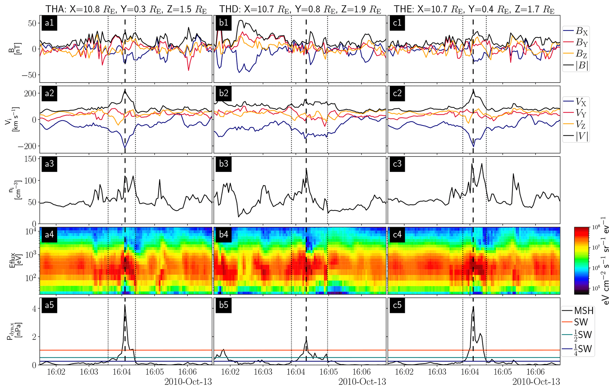
Figure 1Plasma jet observed by the three THEMIS spacecraft THA (a), THD (b) and THE (c), respectively. From top to bottom, the magnetic field and ion velocity components in GSE coordinates and their magnitudes, the ion density, the ion energy flux density and the GSE-X component of the dynamic pressure are shown. The vertical dashed lines in each column mark the times of the maximum dynamic pressure ratio (tmax). The dotted lines denote the start (tstart) and end times (tend) of the jet intervals. The horizontal lines in the last row represent the solar wind dynamic pressure as well as half and a quarter thereof (in orange, cyan and blue, respectively).
The ion energy flux density (Fig. 1a4–c4) and the high ion density (Fig. 1a3–c3) clearly show that all three spacecraft are in the magnetosheath at the time of the event. The positions in GSE coordinates are given above each column of the figure; they show that all the spacecraft are close to the Sun–Earth line. The dynamic pressure (Fig. 1a5–c5) exhibits a clear increase above the solar wind value for all the spacecraft, ensuring that we are indeed observing a jet. The times tmax are separated by only 13 s, and the dynamic pressure peaks resulted from a combined increase in ion density and Vx for every spacecraft. The increase in density is rather high compared to the statistics presented in Plaschke et al. (2013), as we observe an increase of about 100 %–200 % from the ambient magnetosheath to the jet core around tmax. Although the velocities appear relatively low, they are still greater than half of the solar wind velocity while we are closer to the magnetopause.
A closer look at Fig. 1 shows a certain correlation of the individual components of the magnetic field B and the ion velocity V at THA and THE (Pearson correlation coefficients are between −0.34 and 0.92). Since the plasma beta is on the order of 10 within the jet and even higher outside, we can assume that the magnetic field lines align with the jet plasma flow, as discussed in Plaschke et al. (2020b). Outside the jet, in the ambient magnetosheath, the correlation is significantly lower (between −0.13 and 0.55).
Raptis et al. (2022a) showed by investigating the velocity distribution function (VDF) that jets may contain a mixture of two plasma populations. In a similar manner, we integrated the 3D VDF over two velocity axes to obtain a 1D VDF along the third velocity component. This is shown in Fig. 2 for the time tmax for all three velocity components of THA, THD and THE.
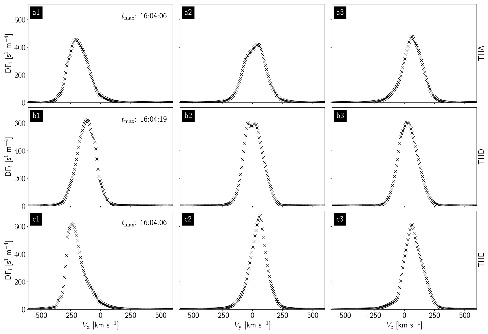
Figure 2The integrated 1D velocity distribution function along the velocity components at the time of maximum dynamic pressure tmax. The columns from left to right represent the Vx, Vy and Vz components, respectively. The rows from top to bottom show the results for THA, THD and THE, respectively. In the left column we denote the time tmax for each spacecraft.
The rows from top to bottom show the VDFs for THA, THD and THE, respectively, and the columns from left to right represent the Vx, Vy and Vz components, respectively. We notice, in agreement with Raptis et al. (2022a), that the Vy component (VDF) of THD (see Fig. 2b2) shows two separate maxima. In addition, the Vx and Vy components deviate from the ideal Maxwellian distribution. THA and THE measurements exhibit only single peaks in the 1D VDFs but also deviate from the ideal Maxwellian distribution (see Fig. 2a1–a3 and c1–c3). The deviations of the 1D VDFs from the ideal Maxwell curve could indicate that all three spacecraft are observing a mixture of jet and magnetosheath plasma. As THD is further away from the other two spacecraft and observes a lower dynamic pressure, we assume THD to be closer to the edge of the jet. It is even possible that THD does not observe the jet but the ambient magnetosheath, because the peak velocity in Fig. 2b1 is comparable to the background velocity in THA and THE (Fig. 2a1 and c1).
Therefore, we continue our analysis only for THA and THE by determining their jet velocities from the 1D VDFs similarly to Raptis et al. (2022a) in the following manner: we examine the 1D VDFs at each time point and use the Vx, Vy and Vz values at which the 1D VDFs have their maximum. If we observe deviations from the ideal Maxwellian (e.g., Fig. 2a1 or Fig. 2c1), we choose the highest absolute velocity in the x direction and the velocity of the coldest population for the y and z directions. We justify this procedure because the deviations from the ideal Maxwellian distribution indicate multiple plasma populations that may influence the moment calculations (for the influence of a background population on the moment calculation, see Raptis et al., 2022a).
To facilitate the analysis of the measurements, we need to define a coordinate system that is aligned with the direction of the jet propagation. As the velocities are rather turbulent, we choose a short time (12 s) centered around tmax and investigated the velocity directions (from the 1D VDFs) measured by THA and THE to determine the propagation direction. For an easier comparison of the directions, we use spherical coordinates with the polar angle Θ and the azimuthal angle φ to visualize the direction of the velocities:
The results are shown in Fig. 3, where the crosses in red, orange and blue represent the measurements of THA, THD and THE, respectively. THD deviates strongly from THA and THE and is only shown for completeness. The black dot represents the mean value of the THA and THE measurements.
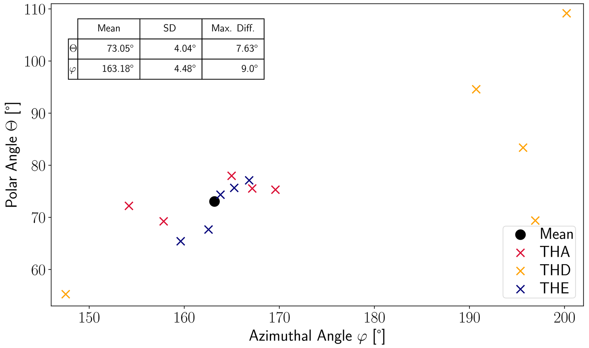
Figure 3The polar angle Θ plotted against the azimuthal angle φ for velocity measurements of THA, THD and THE around tmax in red, orange and blue, respectively. The black dot represents the mean value of the THA and THE measurements. The table in the upper right shows the mean values, standard deviations and maximum differences of Θ and φ.
The directions of THA and THE are more similar and do not vary significantly around tmax. We therefore can assume that the mean values of Θ = 73.05° and φ = 163.18° represent the propagation direction Vjet well. In addition, we also calculate the standard deviation (Θ=4.04°, φ=4.48°) and maximum difference from the mean (Θ=7.63°, φ=9.00°). To treat the uncertainty of the propagation direction conservatively, we will use the maximum differences as error estimation. With the mean values for Θ and φ, we determine the propagation direction (in GSE coordinates) and calculate the axes of the new coordinate system as follows:
eX is the unit vector along the GSE-X axis. points in the propagation direction of the jet, while and are oriented perpendicular to the propagation direction and complete the right-handed system. We choose the position of spacecraft THA at tmax (see the top of Fig. 1) as the origin of our jet coordinate system since THA observes the highest dynamic pressure. To transform the velocities and positions, we simply rotate them into the new coordinate system.
Using the jet coordinate system, we can investigate the flow patterns at the spacecraft positions. This is shown in Fig. 4, where the arrows indicate the ion velocities (from the 1D VDFs) at the spacecraft positions (circles) of THA, THD and THE in red, orange and blue, respectively. The figure shows the orientation of the velocities in the plane, perpendicular to the propagation direction, for 11 time steps from 15 s before to 15 s after tmax. The Y′ and Z′ axes are identical for each time step.
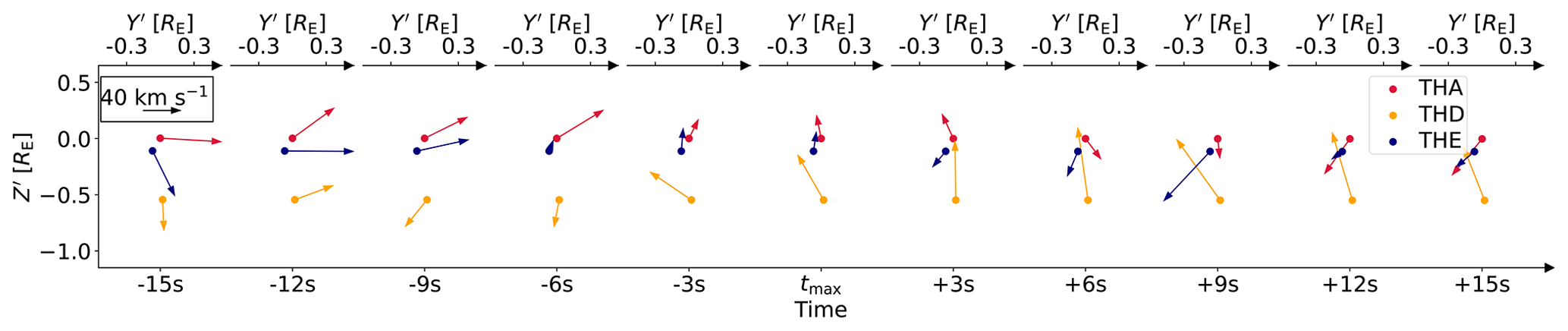
Figure 4Ion velocities from the 1D VDFs at the three spacecraft positions for 11 time steps around tmax in the plane perpendicular to the jet propagation direction. The circles represent the spacecraft positions and the arrows indicate the velocities. The colors for THA, THD and THE are red, orange and blue, respectively. The top axis shows the corresponding Y′ coordinates for each time step, while the bottom axis displays the time steps. In the upper-left corner, the black arrow indicates the scale.
Plaschke and Hietala (2018) reported that the vortical motion of the plasma is not only visible outside of the jet, but is also apparent within the jet structure. Therefore we choose this time range where all spacecraft observe the jet. We remind the reader that we will primarily focus on THA and THE as we have already discussed that THD is farther away from the other two spacecraft and might observe a mixture of plasma populations or even just the ambient magnetosheath. That said, we argue that the following description also applies to THD, but we expect deviations from the general behavior as the conditions are different compared to THA and THE.
On the left side of Fig. 4, prior to tmax, the arrows point towards the positive Y′ direction but in different Z′ directions. We interpret these as signs of diverging flow. Closer to tmax, from 3 s before to 9 s after tmax, the arrows show a rather turbulent behavior, and we observe rotations of the arrows, mostly in the counterclockwise direction. Looking at Fig. 1a5 and c5, we see two high dynamic pressure peaks in this time interval at THA and THE. In contrast, the arrows on the right side in Fig. 4, from −12 to −15 s, corresponding to times after tmax, point towards the negative Y′ direction. The arrows point additionally towards roughly one point and show signs of a converging plasma flow.
In Appendix A we show that the visibility of this vortical motion is not strongly dependent on the propagation direction, as the same flow patterns are still visible at THA and THE for slightly rotated coordinate systems that are consistent with the determined uncertainties.
Next we determine which regions of the jet the spacecraft observe. In order to achieve this, we use the diverging flows before and the converging flows after tmax to estimate the position of the central axis of the jet. Thereafter, we can calculate the spacecraft distances from the central axis within different cross sections of the jet.
We extend the THA and THE velocity vectors in the plane and determine the central axis as the point where the two lines intersect. As an example, in Fig. 5a, b we show the estimation for the time steps 12 s before and 15 s after tmax. The gray lines indicate the extension of the velocity vectors and the black cross represents the estimated position of the central axis. In Fig. 5c we present the estimated positions of the central axis for all the time steps, except where we observe the largest dynamic pressures (from 3 s before to 9 s after tmax).
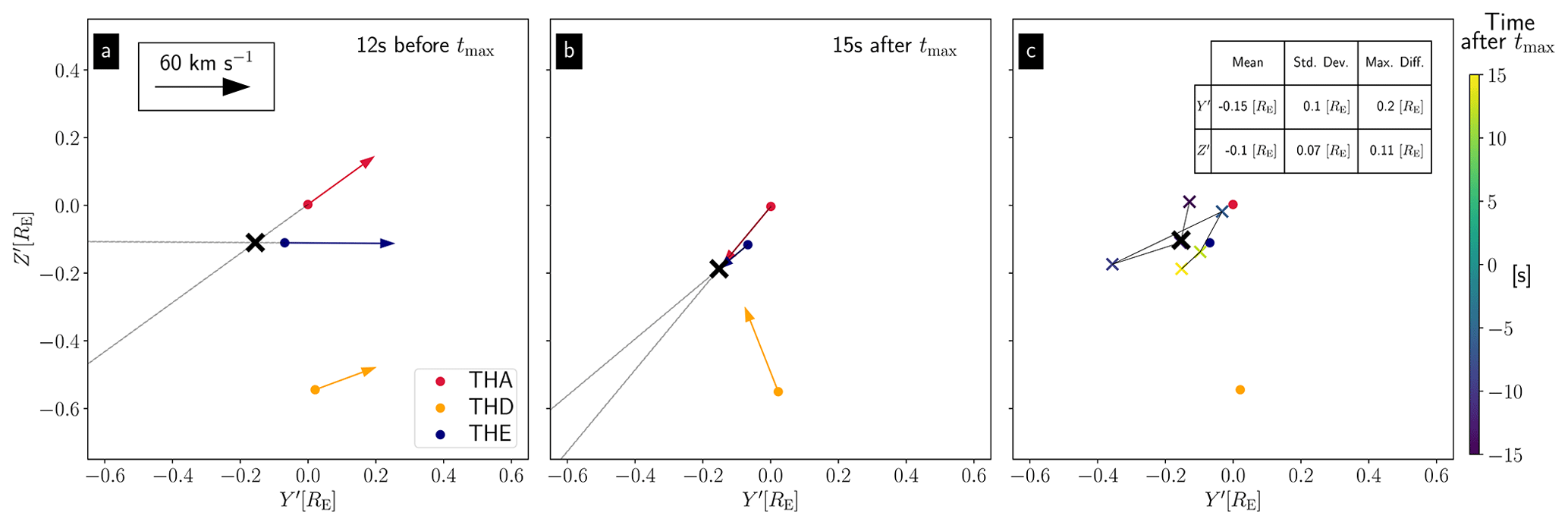
Figure 5(a, b) Ion velocities from 1D VDF peaks at the three spacecraft positions 12 s before (a) and 15 s after tmax (b) in the plane perpendicular to the jet propagation. The circles represent the positions of the spacecraft and the arrows indicate the velocities. The colors for THA, THD and THE are red, orange and blue, respectively. The black arrow indicates the scale. The gray lines are simple extensions of the velocity vectors, and the black crosses mark the intersections of the lines, representing the estimated center positions. (c) The colored crosses show the estimated positions for different time steps. The color corresponds to the time as indicated by the color bar. The black cross represents the mean value, and the dots in red, orange and blue are the positions of THA, THD and THE, respectively. The table in the upper right denotes the mean values, standard deviations and maximum differences of the Y′ and Z′ coordinates.
Based on Fig. 5c, we can calculate the mean position of the central axis: RE and RE. We also observe that the position is relatively well determined, as can be seen by the low standard deviations ( RE, RE) and maximum differences ( RE, RE). Only the estimation at 9 s prior to tmax causes a large error, especially in the Y′ direction. Again, to be conservative, we use the maximum differences as uncertainties and assume the position of the central axis to be valid for the entire jet interval.
In the next section we will use the spacecraft positions and their distances from the central axis to investigate the dynamic pressure profiles for different cross sections. In order to achieve this, we fit a Gaussian distribution that can also be used to estimate the scale size of the corresponding cross section to the Pdyn,x measurements:
Here the parameters P0 and ΔR are the amplitude and width of the Gaussian, and r represents the distance to the central axis. The choice of the Gaussian profile may be somewhat arbitrary. Even though we cannot guarantee that it describes the jets in reality, the measurements in this case are well described by this profile. To apply this fit, we have to assume a monotonous decrease in the dynamic pressure from the center towards the edges in the direction perpendicular to the jet propagation (with increasing r). We furthermore assume a rotational symmetry around the central jet axis to ensure a robust fit. However, we do not make any assumptions for the dynamic pressure along the propagation axis.
Using the estimated position of the central axis, we calculate the distances of the spacecraft from the central axis r in the plane. This results in distances of 0.19 RE, 0.48 RE and 0.09 RE for THA, THD and THE, respectively. These values change only marginally (maximum 3 %) over the jet interval due to the spacecraft movement, assuming the central axis stays constant.
To obtain dynamic pressure profiles, we plot Pdyn,x derived from the velocities from the 1D VDFs in the spacecraft system against the distances r for different times and apply the Gaussian fit. In Fig. 6, we show this for the times tmax−9 s (a), tmax (b) and tmax+15 s (c). Crosses in red, orange and blue represent the data points for THA, THD and THE, respectively. We also plot one-fourth of the solar wind dynamic pressure (blue horizontal line) in Fig. 6a–c, and the Gaussian distribution is shown as black dashed line. The gray area visualizes the standard deviation σ of the optimal fit parameters. Here, σ is the square root of the diagonal elements of the covariance matrix for the fitting parameters.
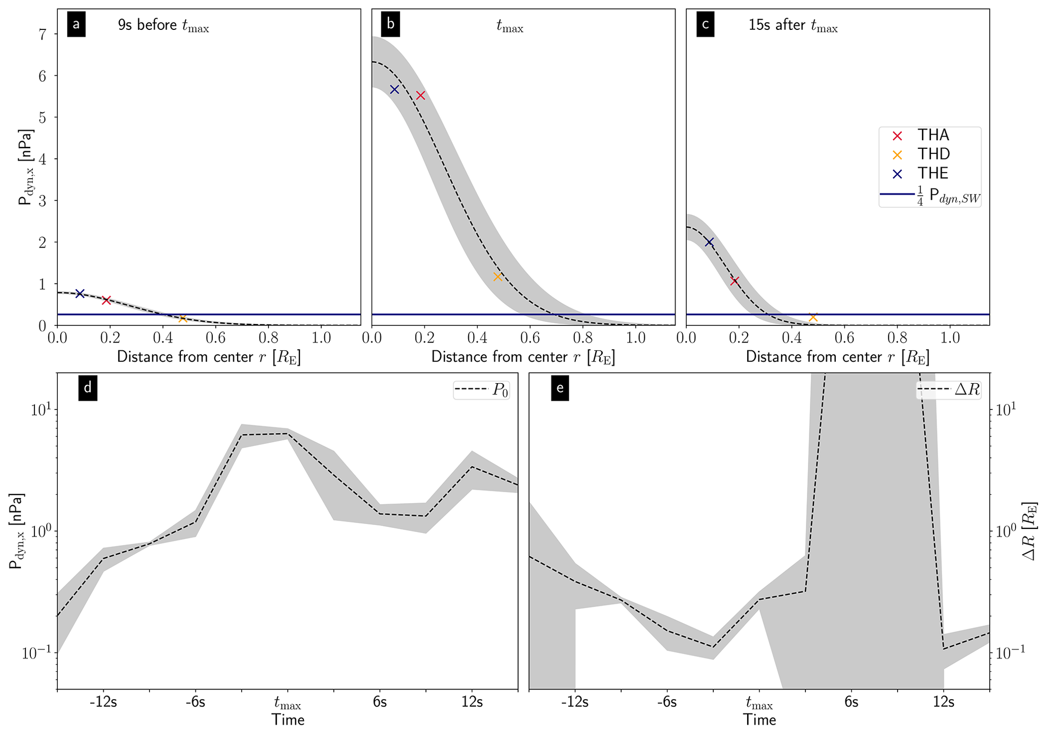
Figure 6Dynamic pressure Pdyn,x derived from velocities from the 1D VDFs in the spacecraft system versus the distance from the center r at THA, THD and THE (crosses in red, orange and blue, respectively) at 9 s before tmax (a), at tmax (b) and at 15 s after tmax (c). The black dashed line represents a fit with a Gaussian distribution to the data points. The blue horizontal line depicts one-fourth of the solar wind dynamic pressure. In panels (d) and (e) we display the development of the fit parameter P0 and ΔR, respectively. The gray areas in all the panels visualize the subtraction/addition of 1 standard deviation σ from/to the optimal fit parameters.
In the three time steps shown, the dynamic pressure is highest at the spacecraft closest to the center (THE). While we see some deviations from the data in Fig. 6b (larger gray area), the fit in Fig. 6a and c represents the data points very well. The fit parameters are P0=0.79 ± 0.02 nPa and ΔR=0.27 ± 0.01 RE at tmax−9 s, P0=6.33 ± 0.60 nPa and ΔR=0.27 ± 0.04 RE at tmax and P0=2.39 ± 0.32 nPa and ΔR=0.15 ± 0.02 RE at tmax+15 s. The estimated central jet dynamic pressure is higher at tmax (6 nPa) than earlier at tmax−9 s (1 nPa) or later at tmax+15 s (2 nPa).
Furthermore, we show the evolution of the central axis dynamic pressure P0 and the width of the Gaussian fit ΔR, obtained by fitting Eq. (3) to the data for the different time steps, in Fig. 6d and e, respectively. In both panels the optimal fit parameters are shown in black, and the gray areas visualize the standard deviation σ of the optimal fit parameters. We observe an increase in the dynamic pressure P0 from tmax−15 s to tmax, followed by a decrease thereafter. In addition, we can recognize a second peak at tmax+12 s, which is already visible in Fig. 1c5 and partially in Fig. 1a5. The increase and decrease in the dynamic pressure along the central jet axis are neither symmetric nor monotonic. The width of the Gaussian profile ΔR shows no clear trend within the jet but two extreme outliers where the fit was not appropriate (6 and 9 s after tmax). At these times, THD observed higher Pdyn,x values than THA despite being farther away from the central axis, resulting in an unrealistic width of the Gaussian fit. On the left side of Fig. 6e, ΔR decreases until 3 s before tmax. It then increases even beyond tmax and is quite low at the end after the two outliers. The uncertainty of ΔR is greater compared to P0, which is indicated by the larger gray area. In contrast, the values of ΔR only vary by about 1 order of magnitude (excluding the two outliers), while the values of P0 change more strongly between approximately 2 orders of magnitude.
The intersection of the fit with nPa leads to an estimation of the jet size in the direction perpendicular to the jet propagation. We choose one-fourth of the solar wind dynamic pressure as a threshold to be consistent with the definitions of tstart and tend for jets, which determine the scale size in the jet propagation direction (see the criterion of Plaschke et al., 2013). The Gaussian fits (black lines) intersect the horizontal line at 0.40 RE, 0.69 RE and 0.31 RE at tmax−9 s, tmax and tmax+15 s, respectively. It is essential to note that both P0 and ΔR contribute to the perpendicular size, and one of them alone cannot describe it. The shape is therefore quite complex, as we observe contrary increases and decreases in P0 and ΔR.
For instance, the width of the Gaussian distribution ΔR is quite similar in the front and central parts, but the higher dynamic pressure in the jet center results in a larger perpendicular size of the jet around tmax. Similarly, the lower dynamic pressure in the front part results in a smaller perpendicular extension. On the other hand, the comparison between the front part (tmax−9 s) and the rear part (tmax+15 s) shows the opposite behavior. We observe a larger perpendicular extension in the front part, although the central dynamic pressure is higher in the rear part. In this case, the greater width of the Gaussian distribution ΔR at tmax−9 s leads to the larger perpendicular size.
We applied the fit here to the measurements from all three spacecraft to reduce the uncertainty of the parameters and to provide an estimate of the uncertainty, which is not possible when fitting to only two data points. However, the qualitative results remain the same if we only use the dynamic pressure measurements from THA and THE. Thus, the possibility that THD is not observing the plasma of the jet but the ambient magnetosheath does not change the conclusions we can draw from our method applied to this jet. In Appendix B we show that the dynamic pressure profiles do not strongly depend on the position of the central axis, as the parameters P0 and ΔR and their evolution over the jet interval vary only marginally with a varying central axis position.
We can compare the estimated scale sizes with previous results. In previous studies, different authors reported a range of scale sizes of magnetosheath jets. Plaschke et al. (2020a) found that most of the jets should be on the order of 0.1 RE, although they argued that these small jets are less likely to be observed. For the observed magnetosheath jets, they reported a median diameter of about 1 RE in the directions parallel and perpendicular to the flow. Gunell et al. (2014) calculated upper limits and found median values of 4.9 and 3.6 RE for the sizes parallel and perpendicular to the flow, respectively. Both studies used pairs of spacecraft and the probabilities that both will observe a jet to calculate sizes perpendicular to the propagation directions. Karlsson et al. (2012) found scale sizes between 0.1 and 10 RE for one direction perpendicular to the magnetic field; for the other two dimensions, the sizes were found to be a factor of 3–10 larger. Thus, our results with diameters of approximately 1.3 RE at tmax and 0.8 RE at times before and after tmax fit very well to the earlier reported sizes.
The method presented by Karlsson et al. (2012) can be used to obtain the sizes of single jets in all three dimensions. This is only possible if the structure is associated with a magnetic field discontinuity, which was the case for all their events. In contrast to this, our method provides scale sizes for the directions parallel and perpendicular to the flow under the assumption of rotational symmetry and a constant propagation direction. We have shown that the latter is given for this jet event to some extent. Furthermore, we assume radial dynamic pressure profiles that resemble Gaussian distributions. The problem can thus be reduced to two dimensions. This enables us to estimate the perpendicular scale size for different cross sections of a jet. Together with the parallel scale size, we could create a simple 3D model of the magnetosheath jet. To apply this method, it is necessary to observe the flow pattern described by Plaschke and Hietala (2018). At least one of the two motions – diverging or converging plasma flow – should be visible to determine the position of the jet's central axis. Observing both parts of the vortical motion leads to more reliable results. This estimation is therefore not applicable to all jets observed by multiple spacecraft, as individual events can deviate strongly from the average behavior. As Plaschke et al. (2020b) have shown for the alignment of velocity and magnetic field, the fluctuations can easily be on the same order of magnitude as the average alignment effect.
Note that the method described in this paper relies on the abovementioned assumptions and simplifications. The choice of the Gaussian distribution for the fit implies a corresponding monotonous decrease in the dynamic pressure from the center towards the edges. These assumptions may not necessarily be satisfied in general or in some parts of the jet. To perform our analysis, we need at least two spacecraft. However, as is evident for this jet event, this is not necessarily sufficient, as the spacecraft should be well separated from each other. More spacecraft observing the same jet or the ambient magnetosheath would allow an evaluation of the validity of our assumptions.
In this paper we demonstrate a new method to determine the size for single jet events using in principle measurements from only two spacecraft. Here we have observed the vortical motion of plasma within a jet with the three THEMIS spacecraft THA, THD and THE. From the diverging flows ahead of and the converging plasma flows behind the jet's maximum dynamic pressure region (at tmax), we were able to estimate the position of the jet's central axis. The distances of the spacecraft from the central axis were used together with the measured Pdyn,x to fit Gaussian distributions. This allowed us to determine the dynamic pressure profiles and the perpendicular sizes of the jet within different cross sections.
Here we have presented dynamic pressure profiles for the jet event for three different times (tmax−9 s, tmax and tmax+15 s). Together with the development of the fit parameters P0 and ΔR, we can draw the following conclusions for this event.
-
The dynamic pressure in the central part of the jet is higher at tmax (6 nPa) and decreases towards the front and rear parts. However, the increase and decrease are neither monotonic nor symmetrical. In addition, we observed a second peak after tmax.
-
The width of the Gaussian distribution and the central dynamic pressure are variable over the jet interval. This results in a rather complex shape with a varying diameter along the propagation axis. We observed the largest perpendicular size at tmax (1.2 RE) due to the high dynamic pressure in the center.
In this paper we cannot explain the asymmetric and non-monotonic increase and decrease in the dynamic pressure along the central axis or the variations in the width of the Gaussian profile. Future work could therefore focus on the evolution of jets and small-scale structures within a jet. However, it may be advantageous or necessary to use spacecraft data with a higher resolution for this task.
The apparent larger scale size around tmax suggests that some spacecraft may only observe central parts of a jet rather than the front and rear parts when passing through edge regions. In addition, spacecraft are unlikely to observe the exact center of a jet. Thus, they would measure just a fraction of the dynamic pressure in the jet center (a lower limit) as Pdyn,x decreases towards the edges, and this would not necessarily be representative for the jet. This implies that statistical studies of dynamic pressures of jets may significantly and systematically underestimate the maximum values (e.g., Raptis et al., 2020). Furthermore, we also emphasize that the comparison of observations with simulations for jets and in general transient and localized phenomena in any plasma environment must take this bias into account.
The jet event selected for this case study belongs to a fraction of jet observations that show clear signs of the expected flow pattern that is needed for the estimation of the central axis. Furthermore, this jet event appears to be quite rare, as we observe very high densities and comparatively low velocities. Other events may differ quantitatively from this case, but we see no reason why it should not work for them. We would like to remind the reader once again that this case study only demonstrates the concept of determining the jet size of individual events and does not claim to determine the general shape of jets.
With only three spacecraft available, there are uncertainties regarding the quality and applicability of the fit and validity of our assumption of rotational symmetry. To increase our confidence in the fit and our assumptions, it would be useful to obtain measurements from even more spacecraft on a jet. This could be achieved through conjunctions of spacecraft from different missions like Cluster (Escoubet et al., 2001), Magnetospheric Multiscale (MMS, Burch et al., 2016) and THEMIS (Angelopoulos, 2008).
The propagation direction of the jet (Vjet) may have a great impact on our analysis. If the direction is incorrect or poorly determined, it is possible that we will not notice the vortical movement even though it is actually present or vice versa. We estimated Vjet as a mean value of multiple measurements by THA and THE. Thus, we imply a constant propagation direction over time and that the velocities at both spacecraft positions represent the propagation well. To handle the uncertainty of these assumptions, we take a look at the maximum differences from the mean velocity (Fig. 3). Adding or subtracting these values to or from Vjet results in Vjet,max and Vjet,min as alternative propagation directions.
With Vjet,max and Vjet,min, we can transform the measured ion velocities and the positions of the spacecraft into new coordinate systems using Eq. (2). We then look at the transformed velocities in the plane (perpendicular to the propagation direction). This is shown in Fig. A1 for Vjet,max in the top row, for Vjet,min in the bottom row and for Vjet in the middle row (for comparison).
We observe the diverging flows before and the converging flows after tmax in all three cases. In addition, we also investigate whether the use of the velocities from the 1D VDFs has an influence on our results. Therefore we use the same propagation directions Vjet,max, Vjet and Vjet,min and transform the ion velocities calculated from the full moments. This is shown in Fig. A2.
Although there are some changes, we can again observe in all cases the diverging flows before and the converging flows after tmax. Thus we conclude that the flow pattern we observe is not an artifact from our data handling.
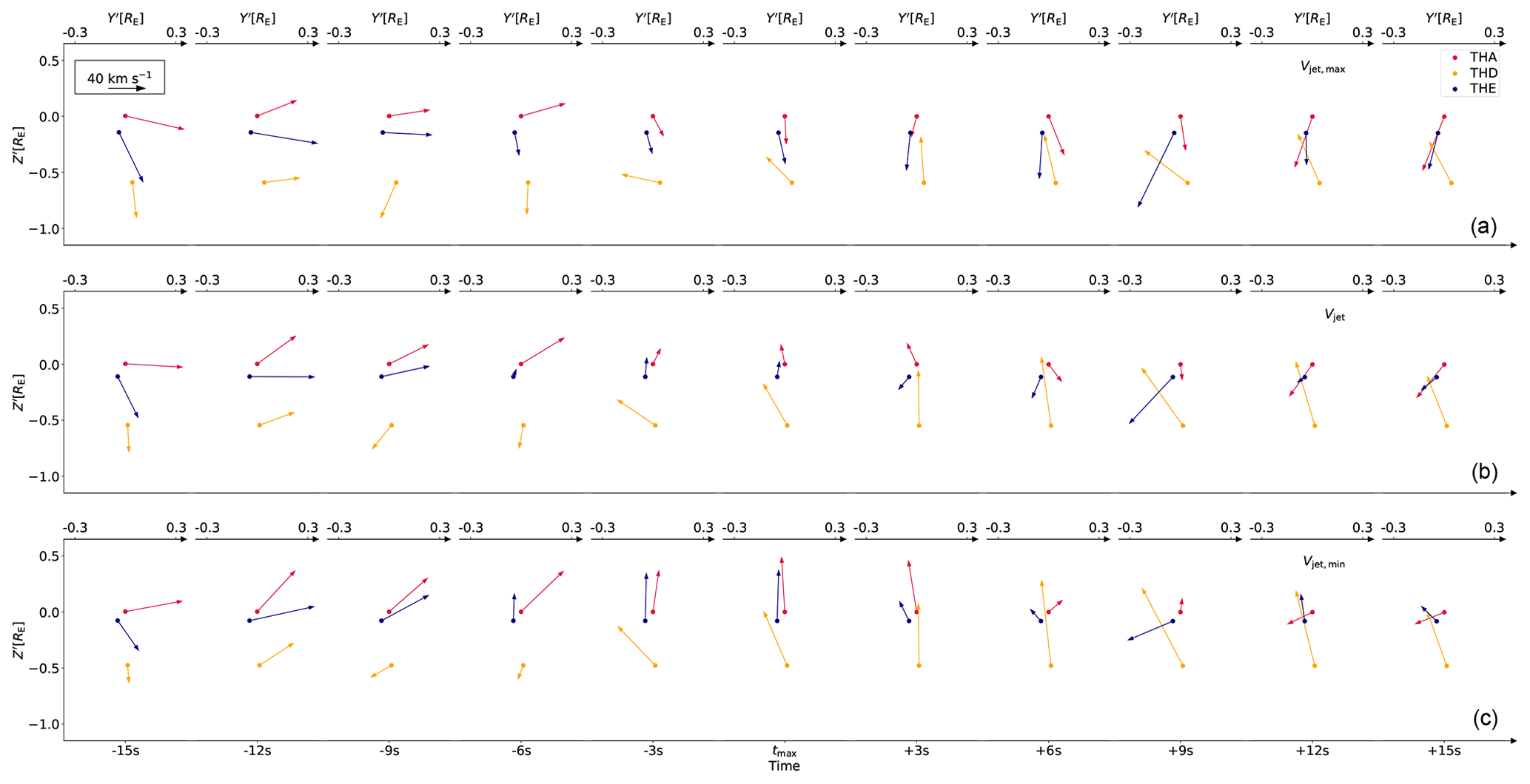
Figure A1Ion velocities from the 1D VDFs at the three spacecraft positions for 11 time steps around tmax in the plane perpendicular to the jet propagation direction. The circles represent the spacecraft positions and the arrows indicate the velocities. The colors for THA, THD and THE are red, orange and blue, respectively. The top axes (a) show the corresponding Y′ coordinates for each time step, while the bottom axis in panel (c) displays the time steps. In the upper-left corner, the black arrow indicates the scale. Panels (a), (b) and (c) were calculated with Vjet,max, Vjet and Vjet,min as propagation directions, respectively.
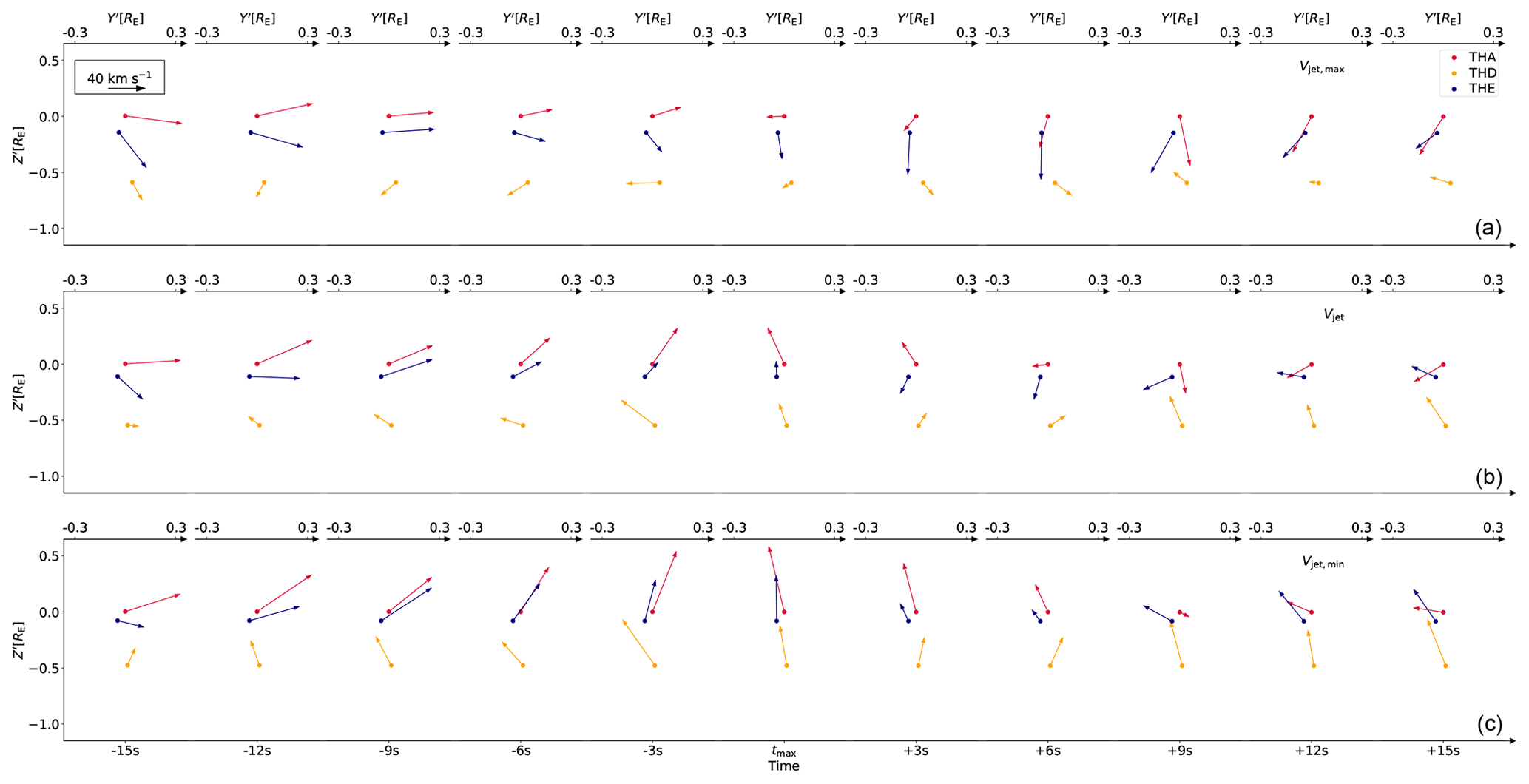
Figure A2Ion velocities from the full moments at the three spacecraft positions for 11 time steps around tmax in the plane perpendicular to the jet propagation direction. The circles represent the spacecraft positions and the arrows indicate the velocities. The colors for THA, THD and THE are red, orange and blue, respectively. The top axes (a) show the corresponding Y′ coordinates for each time step, while the bottom axis in panel (c) displays the time steps. In the upper-left corner, the black arrow indicates the scale. Panels (a), (b) and (c) were calculated with Vjet,max, Vjet and Vjet,min as propagation directions, respectively.
Since THA and THE are close to each other and in the vicinity of the central axis in the plane perpendicular to the propagation direction, minor deviations of the position of this axis can have major effects on the dynamic pressure profiles. Therefore, we use the maximum differences from the mean to calculate alternative positions of the central axis and compare the resulting pressure profiles. In order to achieve this, we look at the fit parameters P0 and ΔR and how these values change with varying central axis positions. In addition, we investigate again whether the use of the velocities from the 1D VDFs has a major influence on the results. Therefore, we calculate Pdyn,x from the velocities from the full moments and repeat the comparison. These results are presented in Fig. B1.
The panels (from top to bottom) show the time evolution of the fit parameters P0 (a1, a2) and ΔR (b1, b2) and the time evolution of their uncertainties σ(P0) (c1, c2) and σ(ΔR) (d1, d2). The left and right columns show parameters for the dynamic pressure calculated with the velocities from the 1D VDFs and with the velocities from the full moments, respectively. The lines represent the results with the mean central axis (solid) and the mean central axis with errors subtracted or added (dotted or dashed).
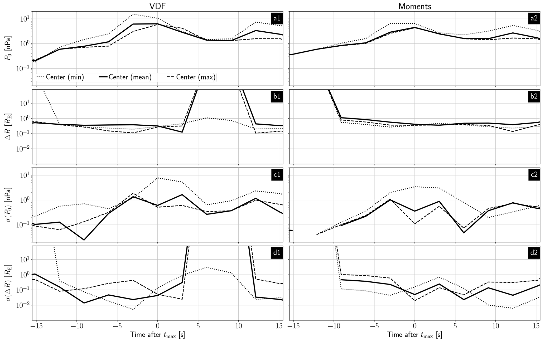
Figure B1The lines represent the results with the mean central axis (solid) and the mean central axis with errors subtracted (dotted) and errors added (dashed). The left and right columns show parameters for the dynamic pressure calculated with the velocities from the 1D VDFs and with the velocities from the full moments, respectively. The panels from top to bottom show the time evolution of the fit parameters P0 (a1, a2) and ΔR (b1, b2) and the time evolution of their uncertainties σ(P0) (c1, c2) and σ(ΔR) (d1, d2).
The dynamic pressure at the central axis is highest around tmax for all cases. We do not observe the second peak at tmax+12 s if we add the errors. Looking at Fig. B1c, we can see that the uncertainty of the fit parameter σ(P0) peaks at tmax−3 and tmax+12 s. The latter may explain why we do not observe the second peak in P0.
For ΔR (Fig. B1c) we observe again a rather similar trend for all cases over the whole time, with some exceptions that correlate well with higher uncertainties in σ(ΔR) (Fig. B1d). These extremely high uncertainties arise when the data do not show a monotonic decrease in dynamic pressure and a Gaussian fit is not appropriate. Therefore, we argue that the exact position of the central axis does not have a major impact on our conclusion.
Data from the THEMIS mission, including level-2 FGM and ESA data, are publicly available from the University of California Berkeley and can be obtained from http://themis.ssl.berkeley.edu/data/themis (THEMIS, 2024). The solar wind data from NASA’s OMNI high-resolution data set (1 min cadence) are also publicly available and can be obtained from https://spdf.gsfc.nasa.gov/pub/data/omni/omni_cdaweb (OMNI, 2024). THEMIS and OMNI data were accessed using the PySPEDAS software (Grimes et al., 2019; Angelopoulos et al., 2019).
AP performed the main work. GG, FK, TK, ZV and FP helped with the discussions and interpretations of the results. JZDM took care of THEMIS FGM calibrations and brought his expertise on THEMIS data to the discussions.
The contact author has declared that none of the authors has any competing interests.
Publisher’s note: Copernicus Publications remains neutral with regard to jurisdictional claims made in the text, published maps, institutional affiliations, or any other geographical representation in this paper. While Copernicus Publications makes every effort to include appropriate place names, the final responsibility lies with the authors.
We acknowledge NASA contract NAS5-02099 for use of data from the THEMIS mission, specifically Charles W. Carlson and James P. McFadden for the use of ESA data; and Karl-Heinz Glassmeier, Hans-Ulrich Auster and Wolfgang Baumjohann for the use of FGM data provided under the lead of the Technical University of Braunschweig and with financial support through the German Ministry for Economy and Technology and the German Center for Aviation and Space (DLR) under contract 50 OC 0302. Florian Koller and Zoltán Vörös acknowledge the support by the Austrian Science Fund (FWF), P 33285-N. The authors want to thank Nick Hatzigeorgiu, Eric Grimes and Jim Lewis for the ongoing development of PySPEDAS.
This work was financially supported by the German Center for Aviation and Space (DLR) under contract 50 OC 2201.
This open-access publication was funded by Technische Universität Braunschweig.
This paper was edited by Oliver Allanson and reviewed by two anonymous referees.
Angelopoulos, V.: The THEMIS Mission, Space Sci. Rev., 141, 5–34, https://doi.org/10.1007/s11214-008-9336-1, 2008. a, b
Angelopoulos, V., Cruce, P., Drozdov, A., Grimes, E. W., Hatzigeorgiu, N., King, D. A., Larson, D., Lewis, J. W., McTiernan, J. M., Roberts, D. A., Russell, C. L., Hori, T., Kasahara, Y., Kumamoto, A., Matsuoka, A., Miyashita, Y., Miyoshi, Y., Shinohara, I., Teramoto, M., Faden, J. B., Halford, A. J., McCarthy, M., Millan, R. M., Sample, J. G., Smith, D. M., Woodger, L. A., Masson, A., Narock, A. A., Asamura, K., Chang, T. F., Chiang, C.-Y., Kazama, Y., Keika, K., Matsuda, S., Segawa, T., Seki, K., Shoji, M., Tam, S. W. Y., Umemura, N., Wang, B.-J., Wang, S.-Y., Redmon, R., Rodriguez, J. V., Singer, H. J., Vandegriff, J., Abe, S., Nose, M., Shinbori, A., Tanaka, Y.-M., UeNo, S., Andersson, L., Dunn, P., Fowler, C., Halekas, J. S., Hara, T., Harada, Y., Lee, C. O., Lillis, R., Mitchell, D. L., Argall, M. R., Bromund, K., Burch, J. L., Cohen, I. J., Galloy, M., Giles, B., Jaynes, A. N., Le Contel, O., Oka, M., Phan, T. D., Walsh, B. M., Westlake, J., Wilder, F. D., Bale, S. D., Livi, R., Pulupa, M., Whittlesey, P., DeWolfe, A., Harter, B., Lucas, E., Auster, U., Bonnell, J. W., Cully, C. M., Donovan, E., Ergun, R. E., Frey, H. U., Jackel, B., Keiling, A., Korth, H., McFadden, J. P., Nishimura, Y., Plaschke, F., Robert, P., Turner, D. L., Weygand, J. M., Candey, R. M., Johnson, R. C., Kovalick, T., Liu, M. H., McGuire, R. E., Breneman, A., Kersten, K., and Schroeder, P.: The Space Physics Environment Data Analysis System (SPEDAS), Space Sci. Rev., 215, 9, https://doi.org/10.1007/s11214-018-0576-4, 2019. a
Archer, M. O., Horbury, T. S., and Eastwood, J. P.: Magnetosheath pressure pulses: Generation downstream of the bow shock from solar wind discontinuities, J. Geophys. Res.-Space, 117, A05228, https://doi.org/10.1029/2011JA017468, 2012. a, b
Archer, M. O., Hietala, H., Hartinger, M. D., Plaschke, F., and Angelopoulos, V.: Direct observations of a surface eigenmode of the dayside magnetopause, Nat. Commun., 10, 615, https://doi.org/10.1038/s41467-018-08134-5, 2019. a
Auster, H., Glassmeier, K., Magnes, W., andW. Baumjohann, O. A., Constantinescu, D., Fischer, D., Fornacon, K., Georgescu, E., Harvey, P., Hillenmaier, O., Kroth, R., Ludlam, M., Narita, Y., Nakamura, R., Okrafka, K., Plaschke, F., Richter, I., Schwarzl, H., Stoll, B., Valavanoglou, A., and Wiedemann, M.: The THEMIS Fluxgate Magnetometer, Space Sci. Rev., 141, 235–264, https://doi.org/10.1007/s11214-008-9365-9, 2008. a
Balogh, A., Schwartz, S. J., Bale, S. D., Balikhin, M. A., Burgess, D., Horbury, T. S., Krasnoselskikh, V. V., Kucharek, H., Lembège, B., Lucek, E. A., Möbius, E., Scholer, M., Thomsen, M. F., and Walker, S. N.: Cluster at the Bow Shock: Introduction, Space Sci. Rev., 118, 155–160, https://doi.org/10.1007/s11214-005-3826-1, 2005. a
Burch, J. L. and Moore, T. E., Torbert, R. B., and Giles, B. L.: Magnetospheric Multiscale Overview and Science Objectives, Space Sci. Rev., 199, 5–21, https://doi.org/10.1007/s11214-015-0164-9, 2016. a
Dmitriev, A. V. and Suvorova, A. V.: Large-scale jets in the magnetosheath and plasma penetration across the magnetopause: THEMIS observations, J. Geophys. Res.-Space, 120, 4423–4437, https://doi.org/10.1002/2014JA020953, 2015. a
Dmitriev, A. V. and Suvorova, A. V.: Atmospheric Effects of Magnetosheath Jets, Atmosphere, 14, 45, https://doi.org/10.3390/atmos14010045, 2023. a
Eastwood, J. P., Lucek, E. A., Mazelle, C., Meziane, K., Narita, Y., Pickett, J., and Treumann, R. A.: The Foreshock, Space Sci. Rev., 118, 41–94, https://doi.org/10.1007/s11214-005-3824-3, 2005. a
Escoubet, C., Fehringer, M., and Goldstein, M.: The Cluster mission, Ann. Geophys., 19, 1197–1200, https://doi.org/10.5194/angeo-19-1197-2001, 2001. a, b
Grimes, E.W., Hatzigeorgiu, N., Lewis, J.W., Russel, C., McTiernan, J.M., Drozdov, A., and Angelopoulos, V.: Pyspedas, a Python Implementation of SPEDAS, Abstract SH41C-3313 presented at 2019 Fall Meeting, AGU, San Francisco, CA, 9–13 December, 2019. a
Gunell, H., Stenberg Wieser, G., Mella, M., Maggiolo, R., Nilsson, H., Darrouzet, F., Hamrin, M., Karlsson, T., Brenning, N., De Keyser, J., André, M., and Dandouras, I.: Waves in high-speed plasmoids in the magnetosheath and at the magnetopause, Ann. Geophys., 32, 991–1009, https://doi.org/10.5194/angeo-32-991-2014, 2014. a, b, c
Han, D.-S., Hietala, H., Chen, X.-C., Nishimura, Y., Lyons, L. R., Liu, J.-J., Hu, H.-Q., and Yang, H.-G.: Observational properties of dayside throat aurora and implications on the possible generation mechanisms, J. Geophys. Res.-Space, 122, 1853–1870, https://doi.org/10.1002/2016JA023394, 2017. a
Hietala, H., Laitinen, T. V., Andréeová, K., Vainio, R., Vaivads, A., Palmroth, M., Pulkkinen, T. I., Koskinen, H. E. J., Lucek, E. A., and Rème, H.: Supermagnetosonic Jets behind a Collisionless Quasiparallel Shock, Phys. Rev. Lett., 103, 245001, https://doi.org/10.1103/PhysRevLett.103.245001, 2009. a
Hietala, H., Partamies, N., Laitinen, T. V., Clausen, L. B. N., Facskó, G., Vaivads, A., Koskinen, H. E. J., Dandouras, I., Rème, H., and Lucek, E. A.: Supermagnetosonic subsolar magnetosheath jets and their effects: from the solar wind to the ionospheric convection, Ann. Geophys., 30, 33–48, https://doi.org/10.5194/angeo-30-33-2012, 2012. a, b
Hietala, H., Phan, T. D., Angelopoulos, V., Oieroset, M., Archer, M. O., Karlsson, T., and Plaschke, F.: In Situ Observations of a Magnetosheath High-Speed Jet Triggering Magnetopause Reconnection, Geophys. Res. Lett., 45, 1732–1740, https://doi.org/10.1002/2017GL076525, 2018. a
Karlsson, T., Brenning, N., Nilsson, H., Trotignon, J.-G., Vallières, X., and Facsko, G.: Localized density enhancements in the magnetosheath: Three-dimensional morphology and possible importance for impulsive penetration, J. Geophys. Res.-Space, 117, A03227, https://doi.org/10.1029/2011JA017059, 2012. a, b, c, d
Karlsson, T., Plaschke, F., Hietala, H., Archer, M., Blanco-Cano, X., Kajdič, P., Lindqvist, P.-A., Marklund, G., and Gershman, D. J.: Investigating the anatomy of magnetosheath jets – MMS observations, Ann. Geophys., 36, 655–677, https://doi.org/10.5194/angeo-36-655-2018, 2018. a
King, J. H. and Papitashvili, N. E.: Solar wind spatial scales in and comparisons of hourly Wind and ACE plasma and magnetic field data, J. Geophys. Res.-Space, 110, A02104, https://doi.org/10.1029/2004JA010649, 2005. a
Koller, F., Plaschke, F., Temmer, M., Preisser, L., Roberts, O. W., and Vörös, Z.: Magnetosheath Jet Formation Influenced by Parameters in Solar Wind Structures, J. Geophys. Res.-Space, 128, e2023JA031339, https://doi.org/10.1029/2023JA031339, 2023. a
LaMoury, A. T., Hietala, H., Plaschke, F., Vuorinen, L., and Eastwood, J. P.: Solar Wind Control of Magnetosheath Jet Formation and Propagation to the Magnetopause, J. Geophys. Res.-Space, 126, e2021JA029592, https://doi.org/10.1029/2021JA029592, 2021. a, b
McFadden, J., Carlson, C., Larson, D., Ludlam, M., Abiad, R., Elliott, B., Turin, P., Marckwordt, M., and Angelopoulos, V.: The THEMIS ESA Plasma Instrument and In-flight Calibration, Space Sci. Rev., 141, 277–302, https://doi.org/10.1007/s11214-008-9440-2, 2008. a
Němeček, Z., S̈afránková, J., Přech, L., Sibeck, D. G., Kokubun, S., and Mukai, T.: Transient flux enhancements in the magnetosheath, Geophys. Res. Lett., 25, 1273–1276, https://doi.org/10.1029/98GL50873, 1998. a
Němeček, Z., S̈afránková, J., Grygorov, K., Mokrý, A., Pi, G., Aghabozorgi Nafchi, M., Němec, F., Xirogiannopoulou, N., and Šimůnek, J.: Extremely Distant Magnetopause Locations Caused by Magnetosheath Jets, Geophys. Res. Lett., 50, e2023GL106131, https://doi.org/10.1029/2023GL106131, 2023. a
Nykyri, K., Bengtson, M., Angelopoulos, V., Nishimura, Y., and Wing, S.: Can Enhanced Flux Loading by High-Speed Jets Lead to a Substorm? Multipoint Detection of the Christmas Day Substorm Onset at 08:17 UT, 2015, J. Geophys. Res.-Space, 124, 4314–4340, https://doi.org/10.1029/2018JA026357, 2019. a
OMNI: Solar wind data from NASA’s OMNI high resolution data set, OMNI [data set], https://omniweb.gsfc.nasa.gov/ow_min.html (last access: 8 March 2024), 2024. a
Palmroth, M., Raptis, S., Suni, J., Karlsson, T., Turc, L., Johlander, A., Ganse, U., Pfau-Kempf, Y., Blanco-Cano, X., Akhavan-Tafti, M., Battarbee, M., Dubart, M., Grandin, M., Tarvus, V., and Osmane, A.: Magnetosheath jet evolution as a function of lifetime: global hybrid-Vlasov simulations compared to MMS observations, Ann. Geophys., 39, 289–308, https://doi.org/10.5194/angeo-39-289-2021, 2021. a
Plaschke, F. and Hietala, H.: Plasma flow patterns in and around magnetosheath jets, Ann. Geophys., 36, 695–703, https://doi.org/10.5194/angeo-36-695-2018, 2018. a, b, c, d, e
Plaschke, F., Hietala, H., and Angelopoulos, V.: Anti-sunward high-speed jets in the subsolar magnetosheath, Ann. Geophys., 31, 1877–1889, https://doi.org/10.5194/angeo-31-1877-2013, 2013. a, b, c, d, e
Plaschke, F., Hietala, H., Angelopoulos, V., and Nakamura, R.: Geoeffective jets impacting the magnetopause are very common, J. Geophys. Res.-Space, 121, 3240–3253, https://doi.org/10.1002/2016JA022534, 2016. a
Plaschke, F., Karlsson, T., Hietala, H., Archer, M., Vörös, Z., Nakamura, R., Magnes, W., Baumjohann, W., Torbert, R. B., Russell, C. T., and Giles, B. L.: Magnetosheath High-Speed Jets: Internal Structure and Interaction With Ambient Plasma, J. Geophys. Res.-Space, 122, 10157–10175, https://doi.org/10.1002/2017JA024471, 2017. a
Plaschke, F., Hietala, H., Archer, M. O., Blanco-Cano, X., Kajdič, P., Karlsson, T., Lee, S. H., Omidi, N., Palmroth, M., Roytershteyn, V., Schmid, D., Sergeev, V., and Sibeck, D.: Jets Downstream of Collisionless Shocks, Space Sci. Rev., 214, 81, https://doi.org/10.1007/s11214-018-0516-3, 2018. a
Plaschke, F., Hietala, H., and Vörös, Z.: Scale Sizes of Magnetosheath Jets, J. Geophys. Res.-Space, 125, e2020JA027962, https://doi.org/10.1029/2020JA027962, 2020a. a, b, c, d
Plaschke, F., Jernej, M., Hietala, H., and Vuorinen, L.: On the alignment of velocity and magnetic fields within magnetosheath jets, Ann. Geophys., 38, 287–296, https://doi.org/10.5194/angeo-38-287-2020, 2020b. a, b, c
Raptis, S., Karlsson, T., Plaschke, F., Kullen, A., and Lindqvist, P.-A.: Classifying Magnetosheath Jets Using MMS: Statistical Properties, J. Geophys. Res.-Space, 125, e2019JA027754, https://doi.org/10.1029/2019JA027754, 2020. a
Raptis, S., Karlsson, T., Vaivads, A., Lindberg, M., Johlander, A., and Trollvik, H.: On Magnetosheath Jet Kinetic Structure and Plasma Properties, Geophys. Res. Lett., 49, e2022GL100678, https://doi.org/10.1029/2022GL100678, 2022a. a, b, c, d, e
Raptis, S., Karlsson, T., Vaivads, A., Pollock, C., Plaschke, F., Johlander, A., Trollvik, H., and Lindqvist, P.-A.: Downstream high-speed plasma jet generation as a direct consequence of shock reformation, Nat. Commun., 13, 598, https://doi.org/10.1038/s41467-022-28110-4, 2022b. a
Savin, S., Amata, E., Zelenyi, L., Lutsenko, V., Safrankova, J., Nemecek, Z., Borodkova, N., Buechner, J., Daly, P. W., Kronberg, E. A., Blecki, J., Budaev, V., Kozak, L., Skalsky, A., and Lezhen, L.: Super fast plasma streams as drivers of transient and anomalous magnetospheric dynamics, Ann. Geophys., 30, 1–7, https://doi.org/10.5194/angeo-30-1-2012, 2012. a
Schwartz, S. J. and Burgess, D.: Quasi-parallel shocks: A patchwork of three-dimensional structures, Geophys. Res. Lett., 18, 373–376, https://doi.org/10.1029/91GL00138, 1991. a
Shue, J.-H., Chao, J.-K., Song, P., McFadden, J. P., Suvorova, A., Angelopoulos, V., Glassmeier, K. H., and Plaschke, F.: Anomalous magnetosheath flows and distorted subsolar magnetopause for radial interplanetary magnetic fields, Geophys. Res. Lett., 36, L18112, https://doi.org/10.1029/2009GL039842, 2009. a
Spreiter, J. R., Summers, A. L., and Alksne, A. Y.: Hydromagnetic flow around the magnetosphere, Planet. Space Sci., 14, 223–253, https://doi.org/10.1016/0032-0633(66)90124-3, 1966. a
Suni, J., Palmroth, M., Turc, L., Battarbee, M., Johlander, A., Tarvus, V., Alho, M., Bussov, M., Dubart, M., Ganse, U., Grandin, M., Horaites, K., Manglayev, T., Papadakis, K., Pfau-Kempf, Y., and Zhou, H.: Connection Between Foreshock Structures and the Generation of Magnetosheath Jets: Vlasiator Results, Geophys. Res. Lett., 48, e2021GL095655, https://doi.org/10.1029/2021GL095655, 2021. a
THEMIS: THEMIS mission including level 2 FGM and ESA data, THEMIS [data set], http://themis.ssl.berkeley.edu/data/themis (last access: 8 March 2024), 2024. a
Vuorinen, L., Hietala, H., and Plaschke, F.: Jets in the magnetosheath: IMF control of where they occur, Ann. Geophys., 37, 689–697, https://doi.org/10.5194/angeo-37-689-2019, 2019. a
Vuorinen, L., Hietala, H., Plaschke, F., and LaMoury, A. T.: Magnetic Field in Magnetosheath Jets: A Statistical Study of BZ Near the Magnetopause, J. Geophys. Res.-Space, 126, e2021JA029188, https://doi.org/10.1029/2021JA029188, 2021. a