Impact ionization double peaks analyzed in high temporal resolution on Solar Orbiter

Solar Orbiter is equipped with electrical antennas performing fast measurements of the surrounding electric field. The antennas register high-velocity dust impacts through the electrical signatures of impact ionization. Although the basic principle of the detection has been known for decades, the understanding of the underlying process is not complete, due to the unique mechanical and electrical design of each spacecraft and the variability of the process.

We present a study of electrical signatures of dust impacts on Solar Orbiter's body, as measured with the Radio and Plasma Waves electrical suite. A large proportion of the signatures present double-peak electrical waveforms in addition to the fast pre-spike due to electron motion, which are systematically observed for the first time. We believe this is due to Solar Orbiter's unique antenna design and a high temporal resolution of the measurements. The double peaks are explained as being due to two distinct processes. Qualitative and quantitative features of both peaks are described. The process for producing the primary peak has been studied extensively before, and the process for producing the secondary peak has been proposed before (Pantellini et al., 2012a) for Solar Terrestrial Relations Observatory (STEREO), although the corresponding delay of 100–300 µs between the primary and the secondary peak has not been observed until now.

Based on this study, we conclude that the primary peak's amplitude is the better measure of the impact-produced charge, for which we find a typical value of around 8 pC. Therefore, the primary peak should be used to derive the impact-generated charge rather than the maximum. The observed asymmetry between the primary peaks measured with individual antennas is quantitatively explained as electrostatic induction. A relationship between the amplitude of the primary and the secondary peak is found to be non-linear, and the relation is partially explained with a model for electrical interaction through the antennas' photoelectron sheath.

1 Introduction

Since their first in situ observation, interplanetary dust grains were observed not only with specialized instruments but also as byproducts of other measurements, making dust detections much more abundant. One promising and actively discussed option for auxiliary dust detection of recent years is impact ionization detection with electrical antennas (Meyer-Vernet, 2001; Mann et al., 2014, and references therein). When a spacecraft collides with a dust grain at a relative velocity exceeding a few kilometers per second, the impact releases free charge due to the high energy density present on the impact site (Friichtenicht, 1964). The released charge is quasi-neutral, yet the present fields often act to separate positive and negative constituents quickly, allowing for its effective detection through the signature in the electric field measurement, once separated. How exactly the detection is done depends greatly on the spacecraft's properties, surrounding environment, impact site, and detecting apparatus. In any case, the perturbation of the electric field stays present for less than 1 ms, while the process of charge separation takes even less time. Therefore, fast electrical measurements are needed in order to observe the process closely.

Solar Orbiter is one of the first (Bale et al., 2016; Maksimovic et al., 2020; Mann et al., 2019) missions to include a wave analyzer suite designed with dust detection in mind. Dust impact events are readily recognized based on a characteristic peak (Zaslavsky et al., 2021; Kvammen et al., 2023), yet the analysis and the interpretation of the recorded signals are made difficult by unclear dependence of the process on spacecraft properties, which is also an issue with other spacecraft conducting similar detection (Zaslavsky et al., 2012; Malaspina et al., 2014; Vaverka et al., 2017; Ye et al., 2019; Page et al., 2020; Ye et al., 2020; Zaslavsky et al., 2021; Kellogg et al., 2021; Racković Babić et al., 2022). In the present paper we report the first observation of a double-peak structure (in addition to the fast electron pre-spike) associated with dust impacts recorded with electrical antennas. The double-peak structure is explained as being caused by two charge collection processes happening simultaneously or in a quick succession and analyzed as such.

We structure the article as follows: in this section, we present Solar Orbiter as a dust detector. We inspect the data and describe our findings in Sect. 2. In Sect. 3, we describe the electrical process theoretically and with quantitative estimates as due to two processes. In Sects. 4 and 5, we focus on primary and secondary peaks respectively. We show that the primary peaks are understood with current knowledge, and we discuss potential explanations for the secondary peaks. We summarize in Sect. 6.

1.1 Solar Orbiter as a dust detector

Solar Orbiter is a three-axis stabilized spacecraft, launched on 10 February 2020, orbiting the Sun, with an aphelion near 1 AU and a perihelion shrinking from 0.5 AU to currently 0.28 AU. Solar Orbiter has remained close to the ecliptic plane so far but will be gaining orbital inclination gradually, starting in 2023 and reaching the maximum inclination of 24 ° and possibly 33 ° in the late 2020s.

The area of the Solar Orbiter's body and shield combined is ≈28.4 m². In addition, the backside of the solar panels is conductive and coupled to the body, which adds another 15.1 m² (Zaslavsky et al., 2021). The spacecraft therefore provides ≈43.5 m² of surface sensitive to dust impacts, where, importantly, ≈7.4 m² is taken by the heat shield front side, which is the effective cross section as seen from the Sun. The effective cross section in the ram direction is ≈4 m² (ESA, 2023). We note that the areas are based on a simplified description of the spacecraft as a cuboid with a heat shield, while a portion of the area is covered by insensitive surfaces. Other sensitive surfaces may contribute to the area besides the cuboid. The heat shield is made of calcium-phosphate-coated titanium, while the body is covered with various metallic and non-metallic materials. Which materials are exposed definitely plays a role in the distribution of impact amplitudes, and this is worthy of future investigation.

1.1.1 Radio and Plasma Waves instrument

The Radio and Plasma Waves instrument (RPW) is a combined electric and magnetic suite for an in situ study of fields and waves (Maksimovic et al., 2020). It provides fast electrical measurements with its three rigid conical nickel cobalt alloy antennas, which enable detection of dust impact events. Each of the antennas is 6.5 m long with a near-base diameter of 38 mm and lies in one plane recessed approximately 1 m behind the heat shield; see the diagram in Fig. 1. Though dust impact events might be identifiable in the electrical spectra, the Time Domain Sampler subsystem (TDS) of RPW is the key to a robust analysis (Zaslavsky et al., 2021), since the dust impacts are solitary pulse events which provide little information on spectra.

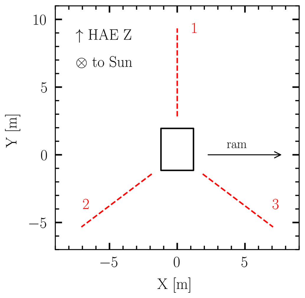
Figure 1 The Solar Orbiter's heat shield (black rectangle) and the RPW antennas (dashed red) viewed in the spacecraft reference frame (from behind).

1.1.2 Radio and Plasma Waves data

The three RPW electrical antennas measure in various configuration modes: monopole, dipole, and mixed. In the monopole configuration, abbreviated SE1, antennas measure voltage against the spacecraft body – this configuration is in principle best suited for dust detection, as the dust impacts' influence on the body potential is of interest. In the dipole mode (DIFF1), antennas measure the electric potential against each other, which has the benefit of the largest effective length for the electrical fields study, but the measurement is nearly insensitive to the changes of the potential of the body. Nonetheless, dust impacts were identified in dipole measurements before and can be identified in DIFF1 measurements of Solar Orbiter, given that the impact influences the potential of an antenna. DIFF1 measurement also provides redundant information on electric fields, as the three antennas lie in a plane; hence only two components could be measured. In the mixed mode (XLD1), the three channels are occupied by two dipoles and a monopole, which in principle retains benefits of both of the aforementioned configurations, as both monopole and dipole signals could be reconstructed. For a more detailed description, see Appendix A. The XLD1 mode is the one that the instrument spends the most time in (≈95.4 %).

The RPW records electrical waveforms with a 6.25 % duty cycle, that is the first 62.5 ms of every second. In trigger mode, the onboard algorithm decides whether to keep each of the recordings, based on the maximum amplitude observed within the window. Up to several hundreds out of approx. 86 400 windows a day are stored and transmitted. The onboard algorithm also classifies the stored waveforms into three different phenomena categories, one of which is the dust impact (more details in Souček et al., 2021). The onboard algorithm, however, does not achieve the precision and accuracy of ground based classifications. In a recent paper, Kvammen et al. (2023) re-did the classification with machine-learning techniques, and this dataset (Kvammen, 2022) is used in the present paper.

Due to technical limitations of the amplifiers, the recorded waveforms can only be trusted within a limited bandwidth. For the purpose of waveform analysis and plotting in the present work, the raw data are altered by a sequence of digital filters to expand this range as much as possible. As a result, the waveforms are trusted in the bandwidth of 500 Hz $<f<$ 70 kHz. For a comprehensive description, consult Appendix B.

2 Observation of impact ionization on Solar Orbiter

Solar Orbiter's RPW electrical antennas (Maksimovic et al., 2020) are similar in terms of construction and the sampling rate to the Solar Terrestrial Observatory (STEREO)/Waves electrical suite (Bale et al., 2008). The antennas are rigid thick poles, with the difference that in the case of STEREO/Waves, the bases of the three orthogonal antennas are physically close to one another, while in the case of Solar Orbiter/RPW, the three antennas lie in one plane, and their bases are physically distant, with the spacecraft's body between them. Nevertheless, the systems' semblance suggests comparable capabilities for dust detection. Therefore, in this section we will present and examine the dust data acquired with Solar Orbiter/RPW, building on the results of and comparing to STEREO/Waves.

2.1 Single and triple hits

STEREO had observed two kinds of dust impact events, so-called single hits and triple hits. The difference is that the triple hits are observed similarly strong on all three channels, which suggests that most of the process takes place on the common ground the channels measure against, rather than on each of the antennas (Zaslavsky et al., 2012). The single hits were reportedly produced by nanodust impacts, which were observed on both STEREO and Cassini with similar fluxes (Schippers et al., 2014, 2015; Meyer-Vernet et al., 2017) when the solar wind electric field focused them towards the ecliptic (Juhász and Horányi, 2013) – a condition that stopped after 2012 (Le Chat et al., 2015). Since they produce small voltages, they were only observed on the antenna lying within the impact cloud, whose voltages could be amplified (Pantellini et al., 2012a; Zaslavsky et al., 2012), and their flux was several orders of magnitude larger than that of beta particles and much more variable, as predicted by Mann et al. (2007). Although STEREO-like single hits are not expected to return until after 2024 (Poppe and Lee, 2020, 2022), it is useful to compare the channels' amplitudes to one another, and we will keep using the terms single and triple hits for Solar Orbiter events, where appropriate. We compare the amplitudes using the ternary plot of channels' maxima, that is the highest amplitude of the voltage between the antenna and the body. The ternary plot is the plot in an equilateral triangle, in which the position in the triangle corresponds to the relative contribution of the three contributors to the sum. In our case, ternary plots are normalized to the sum of three channel maxima for an impact, showing a relative amplitude of the three channel maxima; see Fig. 2.

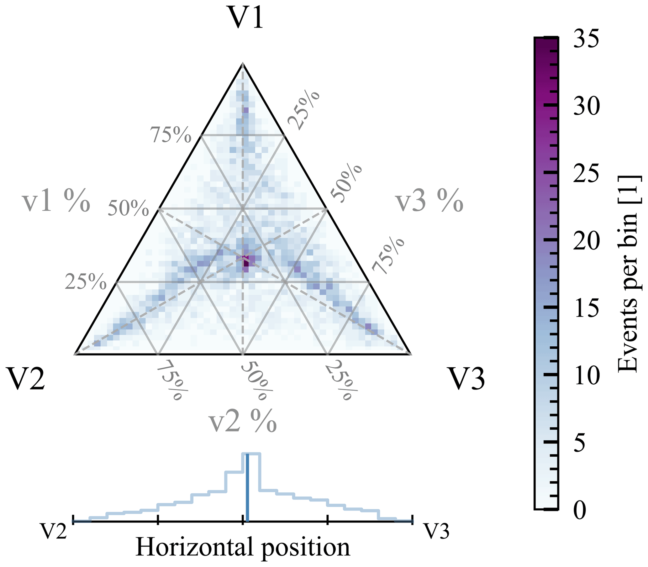
Figure 2 Heat map in the ternary plot for the channel maxima ($VX={\mathrm{ant}}_X-\mathrm{body}$) for all the events identified as dust impacts. 4534 data points contribute to the heat map.

We see that many events lie near the center, which corresponds to a similar response on all three antennas. However, many events lie towards the corners as well, especially near the triangle's medians, which implies an amplitude in one channel higher than in the other two channels, which are in turn nearly equal to one another. This suggests that a process concerning antenna might be present – similar to the conclusion made for STEREO's single hits (Zaslavsky et al., 2012; Pantellini et al., 2012a). The spacecraft has a rough lateral mirror symmetry between antennas 2 and 3, while antenna 1 lies in the plane of symmetry. We see a small preference of antenna 3 against antenna 2, which is to be expected, since antenna 3 is closest to the ram direction, while antenna 2 is close to the anti-ram. The schematic view of the three antennas with respect to the spacecraft body is shown in Fig. 1. We also see that double hits (strong in two and weak in one channel) are not very frequent, but clearly the pair of antenna 3 and antenna 1 is the most prevalent for such hits. This is also to be expected given the direction of the ram. Note that this is a crude representation as it only accounts for the global positive maxima and is therefore an imperfect measure of impact location. Overall, the preference for ram direction is apparent, and a process concerning antennas is hinted at through the presence of single hits.

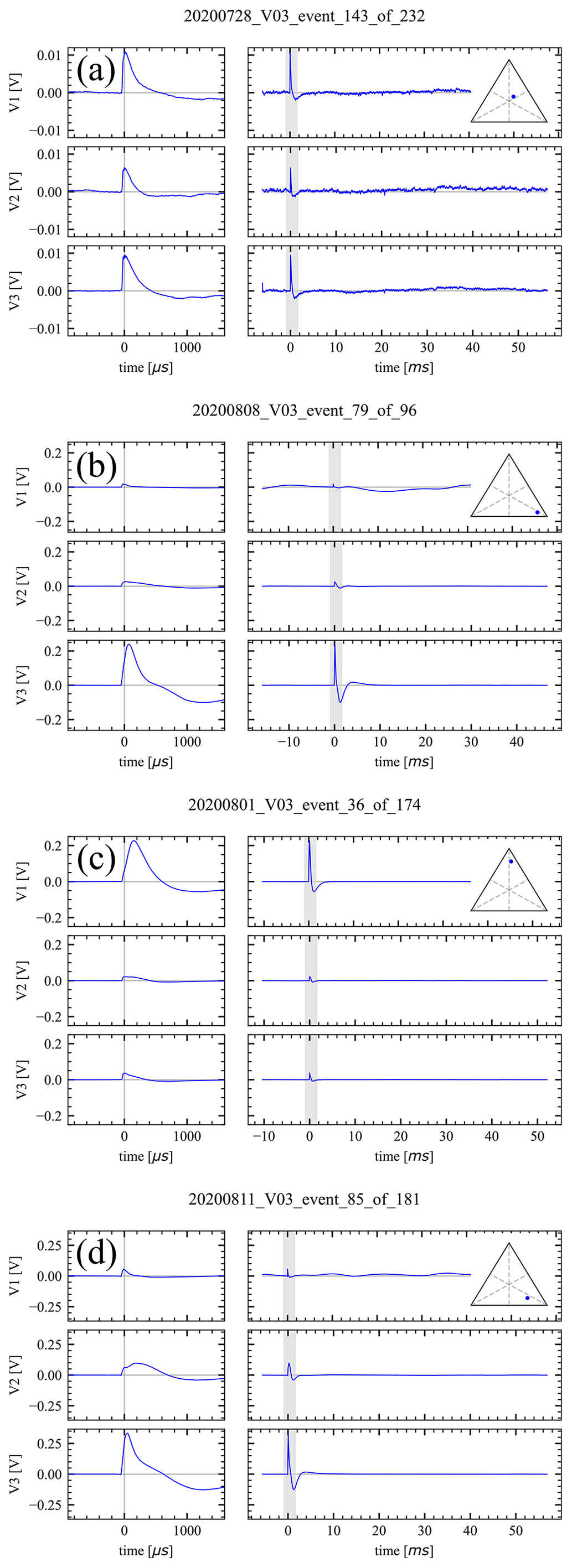
Figure 3 Dust impact events, recorded in true monopole (SE1) mode, corrected (see Appendix B). The voltages are shown as $VX={\mathrm{ant}}_X-\mathrm{body}$. The triangular insets show the corresponding location of the event on the amplitude ternary plot; consult Fig. 2. The left-hand side shows detail of the shaded portion of the right-hand side, which in turn shows the whole recording of 62 ms. (a) A clear triple hit: simultaneous and with similar amplitude in all three channels. (b) Channel V3 shows larger amplitude, compared to channels V1 and V2. A relative delay of ≈50 µs is present. (c) Channel V1 shows larger amplitude, compared to channels V2 and V3. A relative delay of ≈150 µs is present. (d) A common primary peak is visible in channels V1 and V2, a secondary peak is present in V2, and a larger amplitude and a delay are present in V3.

2.2 Waveform inspection

Upon inspection of the corrected signals (see Appendix B) recorded in monopole (SE1) mode (see Fig. 3), we see that many of the waveforms show the following structure: a simultaneous peak of similar amplitude in all three of the channels (Fig. 3a; let us denote the peak a primary peak), often followed by a secondary peak of a different amplitude and delay in each channel, not always present in all of the channels (Fig. 3b, c, d). Sometimes one of the channels shows a more prominent peak instead of the primary peak (Fig. 3d). It seems reasonable to explain these cases as the secondary peak following shortly after the primary peak and hence overshadowing the primary peak. Since it is often the case that just one of the channels shows a secondary peak much stronger than the primary peak (Fig.  3b, c, d), we identify the often-seen single hits as being due to the secondary peak (see Fig. 2 and the corresponding discussion). The two-peak structure is clearly present in many of the impacts (≈50 %), and even more are consistent with the pattern. To the best of our knowledge, this is the first time when such clear double-peak structures in the impact signals were observed. For separate ternary plots for the impacts that do and that do not show double-peak structure, see Appendix C.

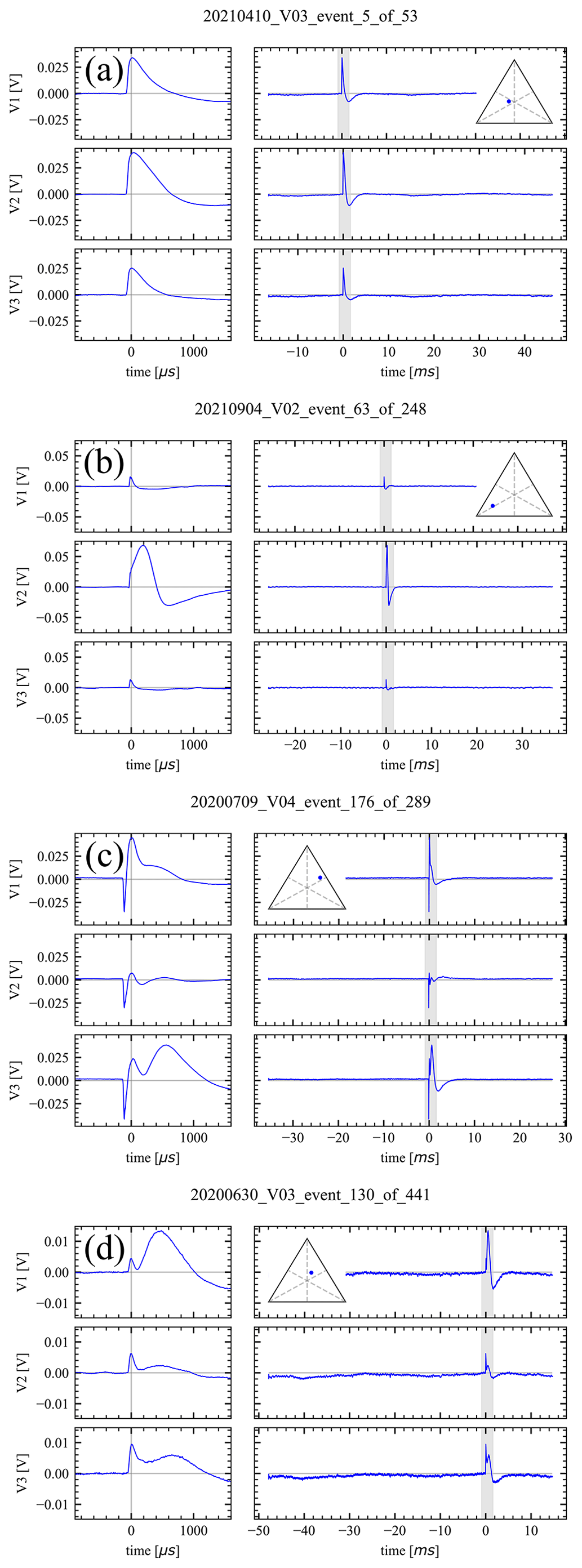
Figure 4 Dust impact events, monopoles reconstructed from signals recorded in hybrid monopole/dipole (XLD1) mode, corrected (see Appendix B). The voltages are shown as $VX={\mathrm{ant}}_X-\mathrm{body}$. The triangular insets show the corresponding location of the event on the amplitude ternary plot; consult Fig. 2. The left-hand side shows detail of the shaded portion of the right-hand side, which in turn shows the whole recording of 62 ms. (a) A clear triple hit: simultaneous and with similar amplitude in all three channels. (b) Channel V2 shows larger amplitude, compared to channels V1 and V3. A relative delay of ≈200 µs is present. (c) A common primary peak is visible all the channels, a secondary peak is present in V3, with hints of it in V1 and V2. A negative pre-spike is clearly present. (d) A common primary peak is visible in all three channels, and a larger amplitude and delay peak are present in V1. Hints of secondary peaks are present in V2 and V3 with different delays.

Signals recorded in mixed (XLD1) mode, decomposed to the monopole channels (see Appendix A) and corrected the same way as monopole signals (see Appendix B), fit the description outlined in the previous paragraph as well (see Fig. 4). This is not surprising, given that the information retained in XLD1 data is virtually the same, except for saturation levels and, to a minor extent, bandwidth. This however confirms that we are justified to treat decomposed XLD1 data the same way as one would treat the monopole signals.

In addition to the primary and the secondary peak, there is often a negative pre-spike present in the waveforms, immediately preceding the main signal. We believe this to be due to electron dynamics, and we will address it in Sects. 3.2 and 4.3.

There is a post-impact negative overshoot present in many of the recordings shown in plots in Figs. 3 and 4. One possible explanation for this behavior was developed and described in Zaslavsky (2015) as being due to a partial collection of the electrons by antennas, that have a longer discharge time constant τ_RC compared to the spacecraft's body. More generally, the behavior is the same, even if the antenna is charged by a different process than the one described by Zaslavsky (2015); that is, the charge does not have to originate directly in the impact plasma. We will not pursue the explanation now, as the tails of the impacts are generally on the edge or outside of the trusted bandwidth, that is, f<500 Hz or τ>2 ms. Let us only note that even though the overshoots are likely distorted and out of scope of this paper, they are likely at least partially physical, as similar overshoots were observed on STEREO (Zaslavsky, 2015) and Parker Solar Probe (Kellogg et al., 2021).

2.3 Features' extraction

For the present analysis, we used the convolutional neural network (CNN)-refined data described in Kvammen et al. (2023), decomposed into monopole signals. In order to describe the events of interest only, that is the body impacts sunlit metallic parts conductively coupled to the spacecraft's body, we employ the following filtering criteria: only the impacts of a maximum amplitude below 0.3 V that are predominantly positive in all the monopole channels were analyzed. The upper limit of 0.3 V is employed in order to avoid reaching the saturation level. We note that predominantly negative pulses produced by antenna hits are also present in the data yet out of scope of the present work, as the electrical process is different for these. Besides, for the sake of data quality, we disregarded the signals captured very near the beginning or the end of the recording window that is within the first or the last 100 samples, or 0.38 ms, since these often do not show the full peaks of interest. After applying these criteria, we are left with ≳50 % of the waveforms in the CNN dataset.

We are interested in the following parameters: amplitude of the primary peak, electron pre-spike presence and amplitude, secondary peaks' presence and amplitudes, and the primary peak's rise and decay times, where the former two peaks (electron and primary peaks) are assumed to be common in all three channels, and the latter (secondary) is analyzed channel-wise. For a comprehensive description of how these are extracted, the reader is referred to Appendix D.

3 Dust impact pulse and process description

Given the previous literature (Friichtenicht, 1964; Auer and Sitte, 1968; Gurnett et al., 1983; Zaslavsky et al., 2012; Pantellini et al., 2012a; Meyer-Vernet et al., 2014; Collette et al., 2015; Meyer-Vernet et al., 2017; Vaverka et al., 2017; Nouzák et al., 2018; Mann et al., 2019; Ye et al., 2019; Kočiščák et al., 2020; Kellogg et al., 2021; Shen et al., 2021b, a; Racković Babić et al., 2022; Shen et al., 2023) and what we observe in the case of Solar Orbiter's RPW data, we formulate a following simplified outlook on the process.

Since the spacecraft is practically always in the sunlight, photoelectrons are released from its body, leading to a positive charge of the most of the spacecraft's body. Upon a hypervelocity dust impact on the spacecraft body, quasi-neutral charge is released. In the case of a spacecraft's body hit, measurement of the spacecraft's antennas potential against its body (Φ_ant−Φ_body) shows an evolution of the voltage difference, summarized on different timescales as follows. The phases numbered (1)–(5) are also visualized in Fig. 5.

1. The impact. A quasi-neutral cloud is born in the near vicinity of the spacecraft. Neglecting a usually small charge possibly carried by the incident dust grain, no change is induced in the spacecraft's potential due to the impact, as the newborn cloud is quasi-neutral, and all the charged particles remain in the near vicinity of each other and therefore have no net influence on the potential. Due to the high density and low mean free path in the newborn cloud, the cloud is at least partially thermalized (Ye et al., 2019; Kočiščák et al., 2020).

2. The electron motion timescale. A portion of the electrons is collected by the spacecraft's body. Simultaneously, a fraction of released electrons with energies high enough to surpass the spacecraft's potential well escapes from the vicinity of the spacecraft. The much slower, net positive ion cloud remains in the vicinity of the impact site. There are two effects going on simultaneously: (a) body potential rises, since the electrons that escaped no longer influence its potential, and (b) antenna potential rises, since neither the escaped electrons nor the electrons collected by the body influence its potential any longer. The latter effect is asymmetric with respect to the three channels, since each antenna is influenced differently, owing to the location of the impact site. The escaping electrons are, however, visible in the form of a symmetric negative spike, owing to the influence of the body potential, possibly forming the aforementioned negative pre-spike. These two (asymmetric positive and symmetric negative) influences counteract each other, and therefore the result is ambiguous, depending on the spacecraft's potential, as well as the instrument geometry and impact site, besides other factors.

3. The timescale of the impact cloud retreating from the vicinity of the spacecraft's surface. As the spacecraft body is positively charged, the net positive impact cloud is repelled. When the impact cloud's electrostatic induction on the body ceases, the electrons previously collected by the body show in the form of a positive peak in the voltage difference, which we denoted as the primary peak. The rise time of the primary peak is therefore the time that ions need to escape far enough from the spacecraft body's vicinity or, alternatively, time until the ion cloud is sparse and far enough so that it is shielded by the photoelectron sheath. The peak is in principle the same on all the channels, since it happens on the body, rather than on the individual antennas. An asymmetry might still be visible due to the electrostatic induction of the ion cloud on the antennas that may not have halted yet, discussed in the previous paragraph. This asymmetry halts on a timescale similar to the rise time of the primary peak, as they both depend on ion motion and shielding.

4. The timescale of the impact cloud reaching the antennas. There is a spike due to ions getting so close to the antennas, that they influence their potential locally. The peak is delayed behind the primary peak due to a finite drift and diffusion velocity of the ions. In fact, the delay of ≳100 µs provides a clear distinction from the induction effect of the ion cloud on the antennas that is observed on a much faster timescale, discussed in phase 2. The antenna charging process is not obvious. Several possibilities for the charging process were previously proposed, observed, and debated.

5. The timescale of potential equalization. Neglecting other influence, the spacecraft's potential is positive and in equilibrium due to balance between the photoelectron current with negative dependence on the spacecraft's potential and the ambient (solar wind) electron collection current with positive dependence on spacecraft's potential. This balance is perturbed by the net negative charge collection from the dust impact, and it is restored on a timescale much more slowly than the impact cloud motion timescale.

Each phase corresponds to one process being dominant; therefore the phases may or may not begin and end with peaks, which depends on amplitudes and timing for the given event. We note that certain phases may or may not be pronounced in individual waveforms, due to a specific voltage balance or phase timing or an insufficient temporal resolution of the waveform sampler. Different behavior may be observed in the case of a less likely impact on a scientific instrument, a non-metallic surface, or a non-illuminated back side of the body. We note that even though the solar panels have a large area compared to the spacecraft's body, they are non-conductive on the front side, which makes them less sensitive to dust impacts. Much is not understood about the panels' response to the impacts, and this is out of scope presently, though it is worthy of future investigation.

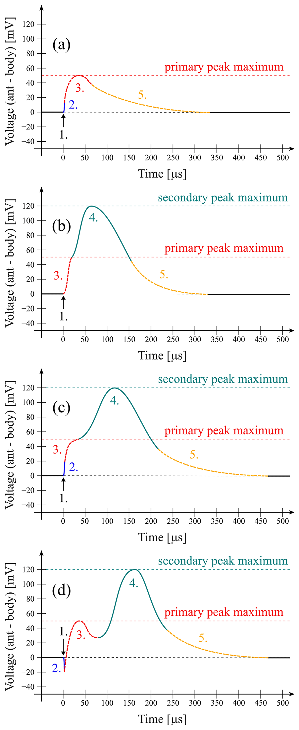
Figure 5 The phases of impact ionization process, as described in Sect. 3. Different eventualities are shown to demonstrate the variability of the pulses that fit the proposed framework. The curves are fictitious, with reasonable primary and secondary peak amplitudes of 50 and 120 mV, as well as a reasonable timescales. The second phase provides an ambiguous step function and is not otherwise related to a specific shape of the curve. Compare to the individual channels in the panels of Fig. 4. (a) No secondary peak is visible; (b) the peaks are discerned by an inflection point; (c) all the phases are clearly visible, although only one local maximum is reached; and (d) all the phases are visible, and two local maxima are reached. The amplitude of the primary peak is 70 mV, rather than 50 mV.

3.1 Charge production equation

The charge is released from the impact site shortly after the dust impact. The amount of charge was found (Auer and Sitte, 1968) to depend on the mass and velocity and is often assumed to follow this empirical equation:

$$\begin{array}{}\text{(1)}& {\displaystyle \frac{Q}{\mathrm{C}}}=A{\left({\displaystyle \frac{m}{\mathrm{kg}}}\right)}^{\mathit{\alpha }}{\left({\displaystyle \frac{v}{\mathrm{km}{\mathrm{s}}^{-\mathrm{1}}}}\right)}^{\mathit{\beta }},\end{array}$$

where m and v are the grain's mass and velocity respectively, and A, α, and β are material constants. We note that the process is stochastic and depends on other parameters, such as the angle of incidence of the impact velocity, so the exact charge can not be reliably predicted, even if these parameters are known, but Eq. (1) was found to work for the mean charge obtained in a repeated experiment. For experimental results and discussion, the reader is referred to Collette et al. (2014) and references therein.

3.2 Electron pre-spike

The negative, electron pre-spike forms due to electrons escaping from the potential well of the positively charged spacecraft. One of the extreme cases is that the potential of the spacecraft is so high compared to the energies of the electrons that virtually no electrons escape, and, hence, no electron peak is observed. In the other extreme case, the potential of the spacecraft is so low that all the electrons moving initially outward (that is, one half of all the electrons) escape. Since the Solar Orbiter operates in the solar wind and in sunlight, its potential does not usually get below +5 V, which means that the latter scenario is unlikely. In reality, values between the two extremes are obtained, leaning towards the former scenario.

3.3 Primary peak

As the Solar Orbiter is typically positively charged to ≈7 V, the positive ions released at the impact are repelled from the spacecraft's body and leave behind the negative charge. It was explained and evaluated before (Zaslavsky et al., 2021) that if the peak is due to a sudden deposition of free charge Q onto the body of the spacecraft, and the antenna's potential ϕ_ant remains roughly constant throughout the process, the peak's amplitude V is linked to the amount of deposited charge as follows:

$$\begin{array}{}\text{(2)}& V\approx {\displaystyle \frac{Q\mathrm{\Gamma }}{C_{\mathrm{sc}}}},\end{array}$$

where C_sc is the electrical capacity of the spacecraft's body (C_sc≈355 pF), while Γ is the capacitive transfer function between the body and the antenna:

$$\begin{array}{}\text{(3)}& \mathrm{\Gamma }={\displaystyle \frac{C_{\mathrm{ant}}}{C_{\mathrm{ant}}+C_{\mathrm{stray}}}},\end{array}$$

where C_ant is the antenna's self-capacitance (C_ant≈55–70 pF, depending on the variable local plasma conditions), and C_stray is the capacitive coupling between the antenna and the body, including the preamplifier capacitance (C_stray≈108 pF). It should be noted that Eqs. (2) and (3) present a simplified outlook, sufficient for our current endeavor. More precise approaches have been taken recently (Shen et al., 2021b; Racković Babić et al., 2022). The approximation requires that the rise of the signal is much faster than the relaxation, which is, as we will see, well met. Then we have Γ≈0.34–0.39. Numbers considered, for the primary peak, we calculate

$$\begin{array}{}\text{(4)}& {\displaystyle \frac{V}{Q}}\approx {\mathrm{10}}^{\mathrm{9}}V/C.\end{array}$$

In their recent modeling effort, Racković Babić et al. (2022) concluded that, in the case of STEREO spacecraft with a similar antenna system, Eq. (2) underestimates the total charge released by about 30 % due to finite rise and finite decay timescales but is a reliable linear measure of the charge released.

We also note that in the case of the presence of the electron peak, we evaluate the amplitude V of the primary peak in reference to the low point of the electron peak, that is to the high point of the spacecraft's potential.

3.3.1 Antenna-induced primary peak asymmetry

In this section, an order-of-magnitude estimate of impact cloud influence on antennas is presented. As explained in Sect. 3, shortly after the impact, electrons are collected by the spacecraft or escape from the cloud of impact-generated plasma. Therefore, the leftover is a net positive charge cloud near the impact site. As the cloud moves away from the impact site, its influence on the body potential gradually ceases, and the primary peak appears, which is the scope of point 3 in Sect. 3. The cloud however influences not only the spacecraft body but also each of the three antennas via induction, as debated in Meyer-Vernet et al. (2014) and Shen et al. (2021a). This influence also ceases once the ion cloud is far away from the spacecraft, but before that happens, this influence is the source of an asymmetry of the primary peak as measured with individual channels, as demonstrated by Shen et al. (2021a). This influence does not require that the ions have moved far from the impact site and is the scope of point 2 in Sect. 3. As an order-of-magnitude estimate, let us study the influence on the antennas' potential if a point charge is located near the heat shield.

Assume a point charge Q at the location x_q and the Debye length of λ_D. The electric potential at the point of space x is then coulombic with Debye shielding:

$$\begin{array}{}\text{(5)}& \mathrm{\Phi }={\displaystyle \frac{Q}{\mathrm{4}\mathit{\pi }\mathit{ϵ}}}{\displaystyle \frac{e^{-\frac{|\mathit{x}-{\mathit{x}}_{\mathit{q}}|}{{\mathit{\lambda }}_{\mathrm{D}}}}}{|\mathit{x}-{\mathit{x}}_{\mathit{q}}|}}.\end{array}$$

The Debye length in solar wind plasma is typically between 3 and 8 m (Guillemant et al., 2013) and hence greater than or similar to the linear dimension of the spacecraft, and the shielding by photoelectron cloud is neglected for simplicity; hence the exponential factor in Eq. (5) is assumed to be equal to unity. A thin antenna (defined by a path l) measures a potential of

$$\begin{array}{}\text{(6)}& {\mathrm{\Phi }}_{\mathrm{ant}}={\displaystyle \frac{\mathrm{1}}{\left|l\right|}}\underset{\mathit{l}}{\int }\mathrm{\Phi }\mathrm{d}\mathit{l}.\end{array}$$

Each antenna responds to the point charge differently, depending on their relative location. The response of the spacecraft's body is assumed as in Eq. (4). Employing a Monte Carlo model for the charge location on the heat shield, we find that the ratio R of primary peak amplitude detected with different channels is up to R≈1.5; see Fig. 6. Similar conclusion can be arrived to based on the results of Shen et al. (2021a), albeit for a different configuration of antennas. For a more detailed description of the model, refer to Appendix F.

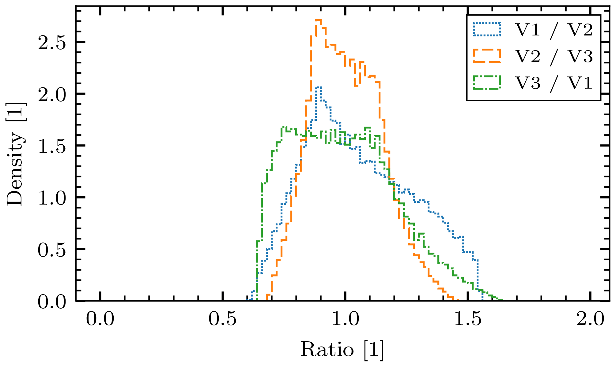
Figure 6 The ratio of primary peak amplitudes as predicted by the model for detection in different channels.

3.4 Secondary peak

Should the antenna get charged, the corresponding voltage would be given by an equation equivalent to the one for the charging of the body but with a different value of the capacitance,

$$\begin{array}{}\text{(7)}& V\approx {\displaystyle \frac{Q\mathrm{\Gamma }}{C_{\mathrm{ant}}}},\end{array}$$

and is hence different by a factor of $C_{\mathrm{sc}}/C_{\mathrm{ant}}$. By substitution for the difference, we find that

$$\begin{array}{}\text{(8)}& {\displaystyle \frac{V}{Q}}\approx \mathrm{6}\cdot {\mathrm{10}}^{\mathrm{9}}V/C.\end{array}$$

It is unlikely that the antenna will get charged by collection of free charges (O'Shea et al., 2017); however the secondary peak might be caused by various mechanisms. Should the antenna only detect the approaching charge remotely (via induction), its response would depend on the geometry of the encounter: the closer the charge gets to the antenna, the stronger the response, with the maximum equal to the charge collection in case of a very close approach. Should the antenna charge due to photoemission (Pantellini et al., 2012a; Kellogg, 2017), the above-mentioned equation holds, and the Q would be the charge due to photoemission. Finally, we note that since the secondary peak is noticeably retarded by ≳100 µs with respect to the primary peak (see Figs. 3, 4), it can not be explained as an electrostatic response to the impact plasma cloud located near the impact site – the motion towards the antenna must be important, and the charging process must be local, requiring proximity of the ion cloud to the antenna. Besides, we observe the electrostatic response as well, on a different timescale, in the form of the primary peak asymmetry.

3.5 Timescales

The electron peak rises when the electrons no longer induce charge on the spacecraft body. It happens no later than when the electrons are displaced from the spacecraft's body by a displacement comparable to the size of the spacecraft body (≈1 m). Consider that the energy of the electrons has to be high enough to overcome the positive potential of the spacecraft's body. The temperature of the impact cloud was estimated before (Friichtenicht et al., 1971; Eichhorn, 1976; Collette et al., 2016; Kočiščák et al., 2020) to be ≳1 eV $k_B^{-\mathrm{1}}$, which implies an electron velocity of v_e≳500 km s⁻¹, leading to a rise time of τ_e≲2 µs, which is well below the 262 ksps resolution of the sampler; hence it appears to be instantaneous. If an electron pre-spike appears to be stronger on certain antennas, it might indicate that it is partially due to electron collection by the antenna.

Similar to the electron peak, the primary peak appears as soon as the released ions no longer induce charge on the spacecraft's body. Two processes cause this: physical displacement of the ions and the shielding of the ions by the electrons (ambient electrons and photoelectrons). Adopting a moderate ion temperature of 5 eV $k_B^{-\mathrm{1}}$ (Collette et al., 2016; Kočiščák et al., 2020) and assuming carbon nuclei, we find the ion speed to be v_i≈9 km s⁻¹. By applying a general electrostatic model for collected and induced charging of all the relevant elements, that is both the antennas and the body of a simplified physical model of a spacecraft, Shen et al. (2021a) measured the speed of ions expanding from a dust impact in laboratory. They found the expansion speed to be $v_{\mathrm{i}}=\mathrm{11.3}\pm \mathrm{0.7}$ km s⁻¹. This value is compatible with the laboratory results of Shen et al. (2021b), who found $v_{\mathrm{i}}=\mathrm{9}\pm \mathrm{1}$ km s⁻¹ using a scaled-down model of Cassini spacecraft. Based on in situ dust impact measurements on Magnetospheric Multiscale (MMS) spacecraft and making use of its tip-sensitive antennas, Vaverka et al. (2021) reported $v_{\mathrm{i}}=\mathrm{27}\pm \mathrm{5}$ km s⁻¹. Recently, Racković Babić et al. (2022) reported 13 km s⁻¹ using a multi-element model applied to STEREO spacecraft's data. Assuming the expansion speed of 10–20 km s⁻¹ we find that the displacement of 1 m occurs in ≈50–100 µs – a time well resolved by the RPW sampler. Should the impact happen within the photoelectron sheath, the photoelectrons are easily the dominant electron population. Assuming typical plasma conditions at 1 AU and an ion speed of v_i=10 km s⁻¹, Meyer-Vernet et al. (2017) estimated the timescale for the shielding of Q=1.6 pC charge to

$$\begin{array}{}\text{(9)}& {\mathit{\tau }}_{\mathrm{ph}}\approx \mathrm{12}\mathrm{\mu }\mathrm{s};{\mathit{\tau }}_{\mathrm{ph}}\propto Q^{\mathrm{1}/\mathrm{3}}{d}^{\mathrm{2}/\mathrm{3}}{v}_{\mathrm{i}}^{-\mathrm{2}/\mathrm{3}},\end{array}$$

which is on the edge of the resolution of the RPW sampler.

The potential altered by the net charge left deposited on the spacecraft's body will decay towards the original spacecraft potential, that is, until the equilibrium is reached again. Under the assumption that the potential perturbation is small compared to the equilibrium potential, the time constant τ_RC of the decay is

$$\begin{array}{}\text{(10)}& {\mathit{\tau }}_{\mathrm{RC}}\approx {\displaystyle \frac{C_{\mathrm{sc}}{k}_B{T}_{\mathrm{ph}}}{e\left|I_{\mathrm{e}}\right|}}\approx {\displaystyle \frac{C_{\mathrm{sc}}{k}_B{T}_{\mathrm{ph}}}{e^{\mathrm{2}}{n}_{\mathrm{e}}{v}_{\mathrm{e}}{S}_{\mathrm{sc}}}},\end{array}$$

where k_BT_ph is the photoelectron temperature (in eV), and $\left|I_{\mathrm{e}}\right|$ is the magnitude of the ambient electron current on the body of the spacecraft, expanded into the product of the charge, density, velocity, and surface en_ev_eS_sc. For details, the reader is referred to Henri et al. (2011). Assuming C_sc=355 pF, k_BT_ph=3 eV, $n_{\mathrm{e}}=\mathrm{5}\times {\mathrm{10}}^{\mathrm{6}}$ m⁻³, v_e=500 km s⁻¹, and S_sc=28.4 m², we get an order-of-magnitude estimate of

$$\begin{array}{}\text{(11)}& {\mathit{\tau }}_{\mathrm{RC}}\approx \mathrm{93}\mathrm{\mu }\mathrm{s}\end{array}$$

for a typical r=1 AU solar wind environment. It is often reasonable to assume $n_{\mathrm{e}}\propto r^{-\mathrm{2}}$.

4 Statistical analysis of the primary peak

The primary peaks are found synchronous and with similar amplitude in all three channels; therefore we believe that the primary peak is the result of the net charge deposition to the spacecraft's body due to impact. In this section, we examine the statistical properties for the primary peaks, such as the distribution of their amplitudes and their rise and decay times. We also compare these to theoretical predictions.

4.1 Amplitude distribution

We analyzed the primary peak amplitudes (as described in Sect. 2.3 and Appendix D) as these are the better measure of the total released charge, compared to the channel global maxima reported previously (Zaslavsky et al., 2021), since the dataset now excludes secondary peaks' amplitudes. The smallest consistently resolved peaks are ≳0.5 mV, and the largest included peaks are amplitudes of ≤0.3 V. Assuming the relation between the primary peak amplitude V and the charge Q in the form of Eq. (4), we find the mean charge to be Q_mean≈21 pC and the median to be Q_median≈8.1 pC. Further discussion is available in Appendix E.

The charge production equation (see Eq. 1) for Solar Orbiter is unknown. We assume a production relation as in McBride and McDonnell (1999), that is $\frac{Q}{C}=\mathrm{0.7}{\left(\frac{m}{\mathrm{kg}}\right)}^{\mathrm{1.02}}{\left(\frac{v}{\mathrm{km}{\mathrm{s}}^{-\mathrm{1}}}\right)}^{\mathrm{3.48}}$, and a mean incident velocity as in Kočiščák et al. (2023), v_mean=63 km s⁻¹. We find the mean incident dust mass $m_{\mathrm{mean}}\approx \mathrm{1.5}\times {\mathrm{10}}^{-\mathrm{17}}$ kg, which corresponds to a spherical dust grain with the diameter of 0.24 µm, assuming the density of ρ=2 g cm⁻³.

4.2 Rise time

We analyzed the rise time of the primary peak and compared it with the estimates presented in Meyer-Vernet et al. (2017) for the case of the sunlit impact surface and for the case of the shaded impact surface (see Sect. 3.5). We adapted the estimates to the median charge of 8.1 pC, as well as the ion speeds of v_i=10 and 20 km s⁻¹, obtained as described in Sect. 3.5. The estimates were done assuming only one (photoelectron shielding or ambient plasma shielding) process, while the other one plays a role as well, as described in Meyer-Vernet et al. (2017) Therefore, even sunlit estimates are overestimates. On the experimental side, the exact definition of the rise time is important, as the rise profile is usually not exponential. In order to exclude a potential fast contribution of the induced charge (as in Sect. 3.3.1), we define the rise time as the time needed to get from $\mathrm{1}/e$ of the maximum to the maximum value of the peak.

Figure 7 shows the dependence of the rise time on the heliocentric distance. Inferred means are close to the theoretical estimate for sunlit surface impact. Figure 8 shows the dependence of the rise time on the primary peak amplitude, assuming heliocentric distance of 0.75 AU. The data show significantly less variation than predicted; however the sunlit estimate is clearly better than the shade estimate. There might be several reasons for the disagreement of the data with the theory. Either the process understanding as in Meyer-Vernet et al. (2017) is incomplete, or there are correlations present between the variables in Eq. (9). We note that several papers (for example, Collette et al., 2016; Nouzák et al., 2020) suggested that the higher impact velocity might lead to a higher ion velocity v_i in addition to a higher charge yield Q, although recent measurements did not observe this (Shen et al., 2021a). If a higher impact speed is correlated with a higher ion expansion speed, then these effects partially counteract each other, and the scaling of the rise time τ_ph is not as in Eq. 9. The theoretical predictions made in Meyer-Vernet et al. (2017) and the ion escape velocity between 10 and 20 km s⁻¹ are compatible with the data with respect to the timescale of the rise time. The theory is also compatible with the variation with the heliocentric distance, though the dependence of the rise time on the impact charge was not observed as predicted, with sunlit estimates providing a better fit to the data, compared to shade estimates.

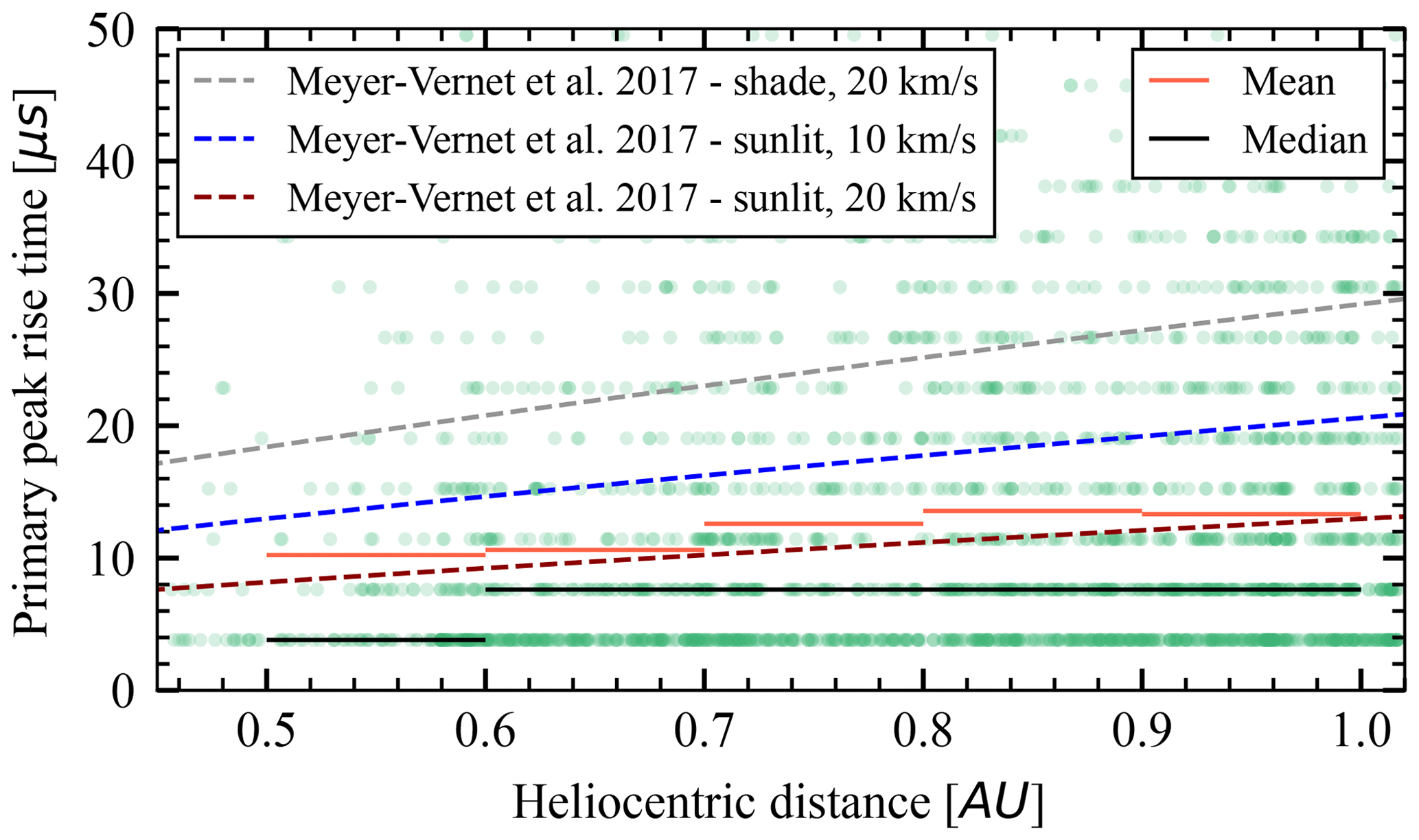
Figure 7 Rise times of the primary peaks as a function of the heliocentric distance. Predictions from Meyer-Vernet et al. (2017) are shown in the case that impact cloud shielding is dominated by photoelectrons (sunlit) or solar wind plasma (shade). The predictions are for the median primary peak's charge of 8.1 pC and for an ion escape velocity of 10 and 20 km s⁻¹.

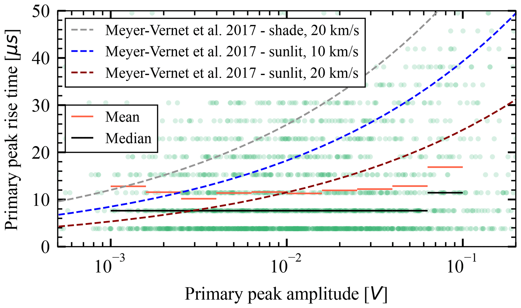
Figure 8 Rise times of the primary peaks as a function of the body's peak amplitude. Predictions from Meyer-Vernet et al. (2017) are shown in the case that impact cloud shielding is dominated by photoelectrons (sunlit) or solar wind plasma (shade). The predictions are for the heliocentric distance of 0.75 AU and for an ion escape velocity of 10 and 20 km s⁻¹.

4.3 Negative pre-spike

The negative pre-spike is present intermittently, for example in Fig. 4c. The presence indicates that a portion of free electrons was able to escape the spacecraft's potential well. We note that the induced charge on the antennas due to the positive impact cloud appears nearly as quickly as the electron pre-spike, and these two effects therefore counteract each other, differently in each channel. The induction on the antennas may be fast and ample enough so that the electron pre-spike is obscured. Concerning the presence and the amplitude of the pre-spike, the exact impact location certainly plays a role, since spacecraft's surface potential is not uniform. On top of that, the spacecraft's potential must play a role as a lower potential implies a shallower potential that electrons need to overcome in order to escape. To see this dependence, we examine the spacecraft potential data product, based on low-frequency receiver measurements of RPW (Maksimovic et al., 2020). We note that this a result of an indirect measurement and therefore the reliability is limited, especially in the case of very high or very low values. A correlation between the pre-spike presence and a relatively lower potential is expected, which is why we show a separate normalized histogram of spacecraft potentials at the times of impacts with pre-spikes and without; see Fig. 9. Pre-spikes are present for nearly any spacecraft potential, but the correlation is apparent, as expected.

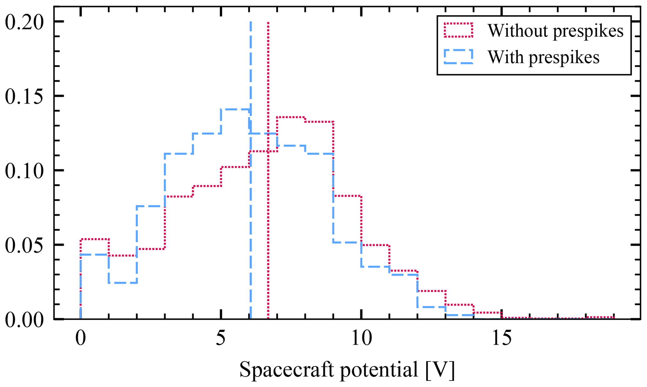
Figure 9 The histogram of spacecraft potential at each dust impact for impact with and without pre-spikes. Averages are shown for the two populations as vertical lines.

4.4 Decay time

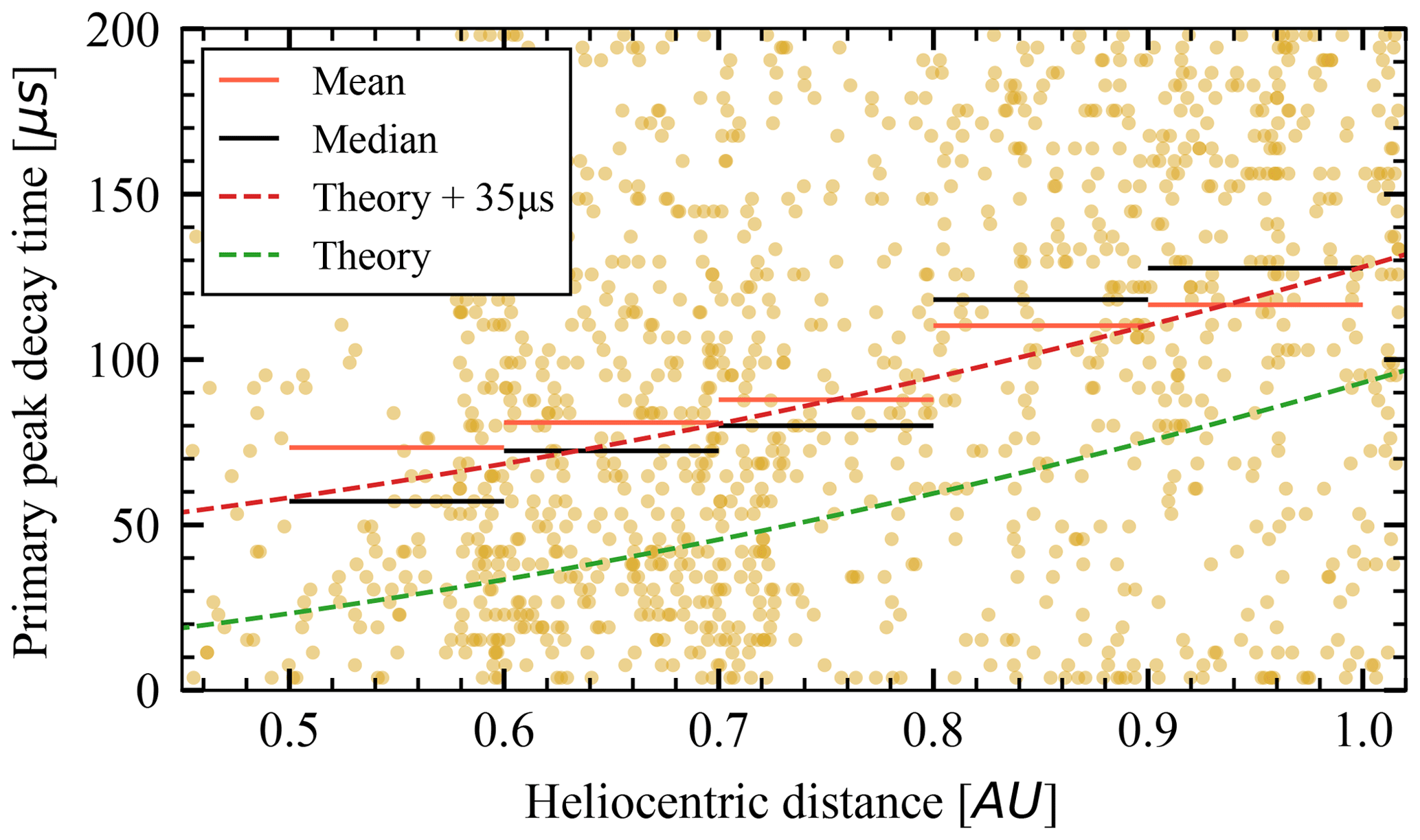
We established the decay time for the primary peaks as the time to get from 100 % to $\mathrm{1}/e$, always for the channel that showed the lowest primary peak amplitude, as that is the one least affected by a possible secondary peak. Furthermore, we disregarded any value over 200 µs for the same reason – if the decay time is very long, it is likely due to the secondary peak. We note that only impact shapes such as in panels (a) and (d) in Fig. 5 allow for this analysis. We compare the result to the theoretical values presented in Sect. 3.5; see Fig. 10. The decay time shows a clear variation, albeit different from the model (Eq. 10). The data show a significant scatter and are compatible with the model with an additional constant offset of around 35 µs. We note that there are uncertainties, for example, in the spacecraft capacitance C_sc and in the spacecraft surface S_sc. The shallower dependence might be a result of electron temperature being higher at lower heliocentric distance, which we do not take into account in the theoretical calculation. We also can not exclude an artifact of the secondary peaks that are present, though not apparent, as these may introduce error that is hard to estimate. The definition of the decay time might play a role, as the decay profile is often non-exponential.

Figure 10 Decay times of the primary peaks as a function of the heliocentric distance.

4.5 Antenna-induced asymmetry

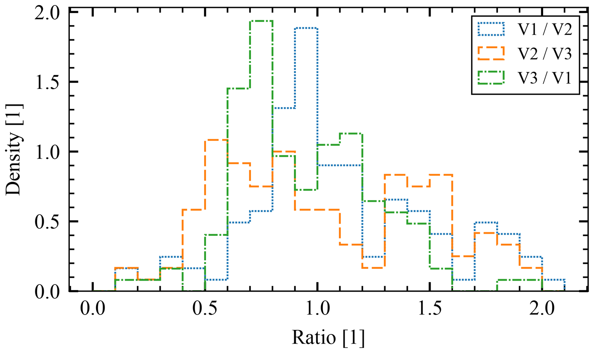
We studied the amplitudes of individual primary peaks in order to compare them to the theoretical predictions of Sect. 3.3.1. We only analyzed the events that show no secondary peak in any channel. In parallel to Fig. 6, ratios of channel pairs are shown in the histogram in Fig. 11. The histogram does not show data with the ratio >2.2, and as a result, 5 of 327 values are not shown. Similarly to the results of the numerical model shown in Fig. 6, values <0.5 are rare, as are the values ≳ 2, which implies that the process as described in Sect. 3.3.1 is a good model for the situation, as it explains the magnitude of observed asymmetry.

Figure 11 Antenna-induced asymmetry to the primary peak's amplitude.

5 Statistical analysis of the secondary peak

An important proportion of the impacts (≈50 %) shows a clear double-peak structure, while even more are compatible with the double-peak structure. The secondary peaks' prominent features include the following:

• strong asymmetry in the three channels,

• intermittent presence,

• variable but pronounced delay with respect to the primary peak.

The first point leads to the conclusion that the process causing secondary peaks mainly takes place on the antennas, rather than on the spacecraft body. This implies that, in the process, the affected antenna is charged more positively. The latter two points imply that the effect relies on a drift of the cations. In this section, we describe statistical properties of the identified secondary peaks.

5.1 Delays

The typical delay lies in the range of 100 µs to 300 µs; see the histogram in Fig 12. The secondary peak's delay varies, nearly uncorrelated with the peak's amplitude or the spacecraft's heliocentric distance; see Figs. 13 and 14. This time is too long to correspond to charge generation, collection, or even equalization due to ambient plasma currents, as we described all of these earlier, and they happen within ≲150 µs.

Figure 12 Histogram of the strongest secondary peak's delay against the primary peak.

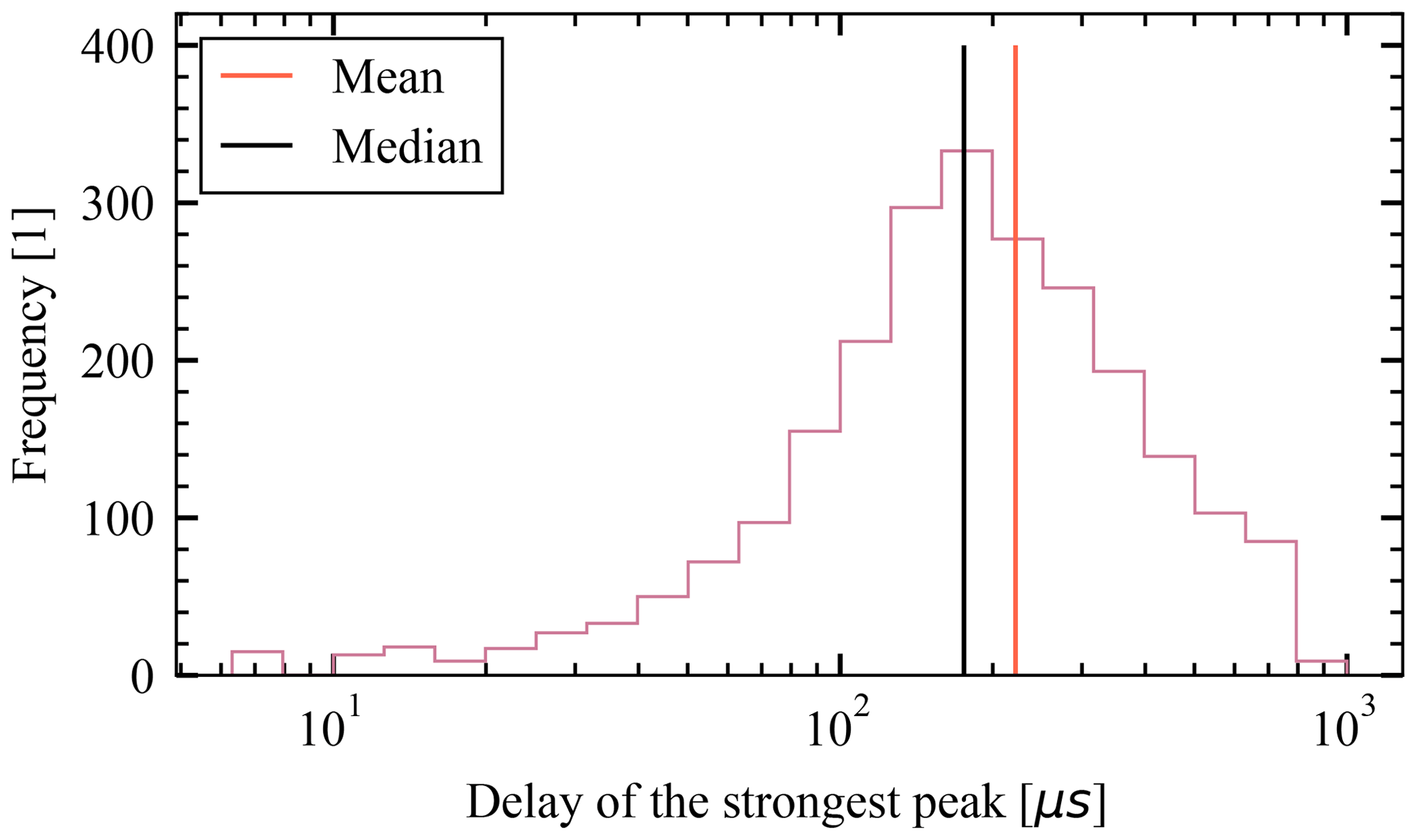
Assuming the ion velocity of 10–20 km s⁻¹ as before, the time delay of 100 to 300 µs translates to 1–6 m of displacement. We note that the Solar Orbiter's heat shield's size is approximately 2.4×3.1 m², and the antennas are 6.5 m long. We therefore conclude that this delay is due to ion motion, since it is the only electric process that happens on this timescale. The fact that no important variation is observed in Fig. 14 suggests that the ion velocity does not vary with the heliocentric distance.

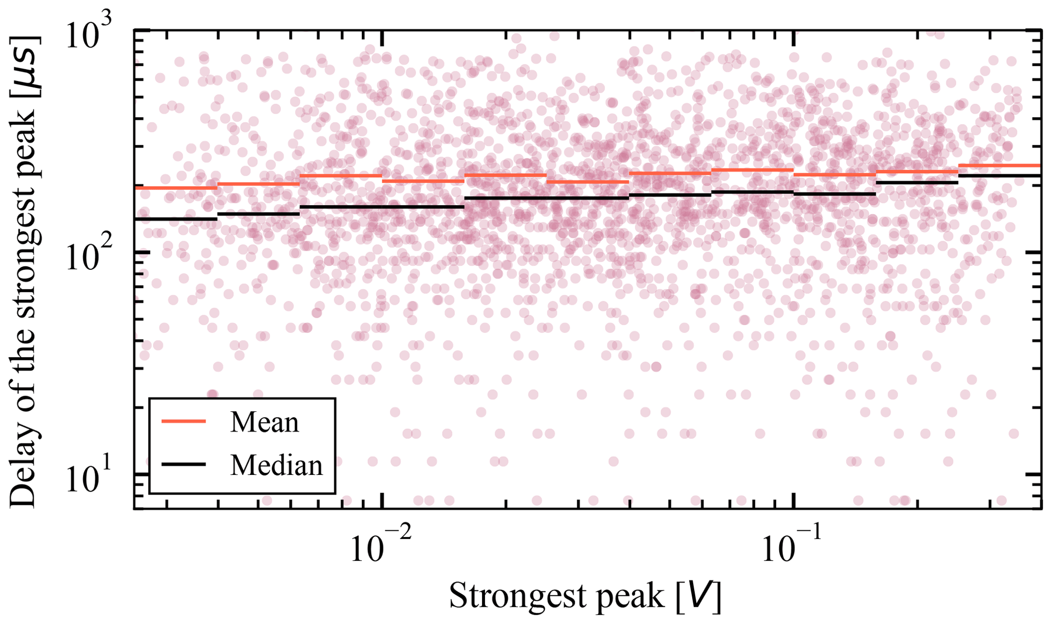
Figure 13 Strongest secondary peak's delay against the primary peak as a function of its amplitude.

We note that the delay of 100 to 300 µs is far enough for the cloud to get shielded by the photosheath, due to its high electron number density (compare with values shown in Figs. 7 and 8). However, the photosheath decays with the distance from the illuminated surface rather quickly, with the typical Debye length of 0.25 m close to Solar Orbiter's perihelia and 1 m close to 1 AU (Guillemant et al., 2013). We therefore come to a conclusion that at least a part of the impact cloud passes through the photosheath (consult Appendix G), and this cloud later influences the antennas. We also note that the photosheath is not uniform and weaker at places that are less illuminated, such as spacecraft sides.

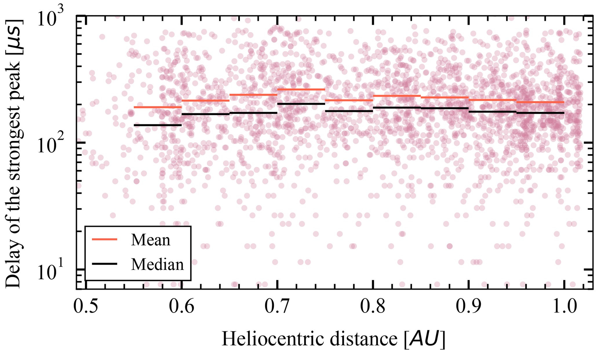
Figure 14 Strongest secondary peak's delay against the primary peak as a function of the spacecraft's heliocentric distance.

The delay does not show variation with the peak absolute amplitude (Fig. 13), but it shows a weak correlation with the amplitude relative to the primary peak amplitude, as is shown in Fig. 15. The primary peak's amplitude is a good measure of the total charge released on the impact, and since we study the secondary peak as a random process, normalization to the impact magnitude is natural.

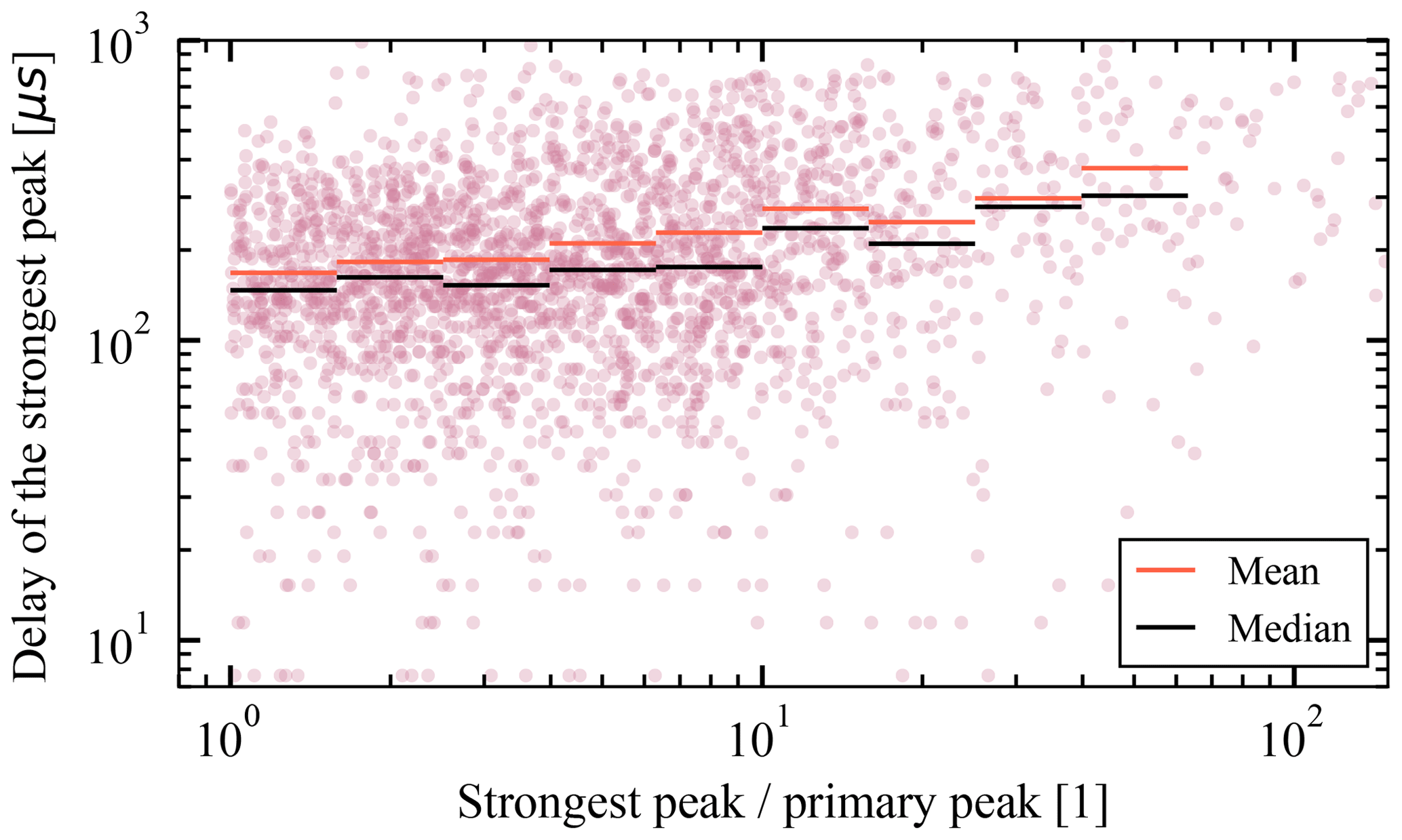
Figure 15 Strongest secondary peak's delay against the primary peak as a function of the strongest secondary peak's amplitude relative to the primary peak.

We also note that the secondary peak is not only delayed; it also evolves and decays on a ≳100 µm timescale, as is apparent from waveforms shown in Figs.3 and 4. This hints that the evolution of the secondary peak is also dependent on the dynamics of the ion cloud's motion. This is also consistent with the positive correlation between the secondary peak's relative amplitude and the delay with respect to the primary peak (Fig. 15).

5.2 Amplitudes

The secondary peak's amplitude varies, and the peak is not always present. We do not claim that small secondary peaks are non-existent; however for the purpose of our analysis, the secondary peaks are considered absent in cases when their amplitudes are much smaller than the primary peak's amplitudes, as then we can not identify them reliably. If the secondary peak is present in a channel, we study its amplitude relative to the amplitude of the primary peak, as the primary peak's amplitude is a good measure of the total charge released on the impact. See Fig. 16 for the plot of relative amplitude of the secondary peak over the primary peak vs. the heliocentric distance in cases where the secondary peak is present. We observe that the typical relative amplitude is between 3 and 5 but often is over 10. There is not a strong correlation between the relative amplitude of the secondary peak and the heliocentric distance.

Given the time delay that corresponds to the ion motion along Solar Orbiter and what was suggested and observed previously with different spacecraft, one may try to explain the secondary peak as the antenna's response to the ion cloud's electric field. This field may be due to the charge separation electric field of the cloud (Oberc, 1996) or due to the different plasma potential within the impact cloud (Zaslavsky et al., 2012). Alternatively, this peak may be due to collection of ions from the impact cloud (Meyer-Vernet et al., 2014; Zaslavsky, 2015; Vaverka et al., 2021; Kellogg et al., 2021). In the extreme case of the collection of all the created ions by a single antenna, the amplitude would be approximately proportional to the amplitude of the primary peak by a factor of $C_{\mathrm{sc}}/C_{\mathrm{ant}}\approx \mathrm{5}$. That is ignoring the fact that the ion cloud is exposed to the solar wind plasma for 100 to 300 µs. The response to the charge collection is also an upper estimate of the response to the induced fields. We also note that a complete collection of the ions by an antenna is unlikely. The reason is that the antennas present a small cross-section for the ions, since they occupy a small solid angle as seen from usual impact site and are metallic and therefore positively charged (O'Shea et al., 2017). Moreover, we often find the secondary peak in multiple channels, which clearly rules out the option that one antenna collects all the ions. Therefore the factor of ≈5 is understood as a very safe overestimate of the secondary peak amplitude, if it is due to the antenna's response to the ion cloud's electric field. As is shown in Fig. 16, the limit of 5 is breached very often, which rules out the linear response of the antenna to the electric field of the escaping ions. The conclusion is that an additional antenna charging process must be present. A similar conclusion was arrived at by Pantellini et al. (2012b) for STEREO spacecraft's single hits.

The capacitance of the antennas and of the spacecraft increase with decreasing heliocentric distance due to photoelectron sheath's presence, but since a greater portion of the antennas is sunlit compared to the spacecraft body, one would expect a positive correlation in the Fig. 16, should the variable capacitance be important, which is not observed.

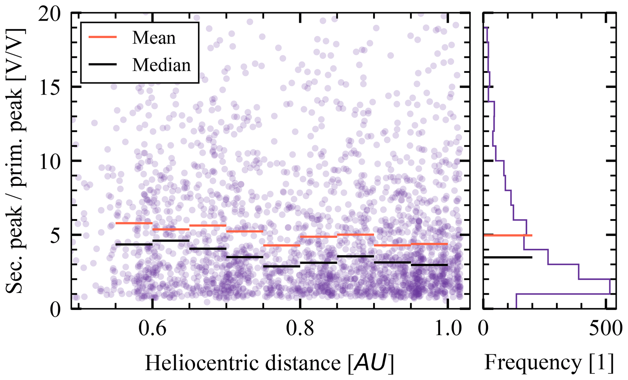
Figure 16 The secondary peak relative to the primary peak as a function of heliocentric distance for the events that show a secondary peak. If the secondary peak is present in multiple channels, the strongest one is shown. The absence of values < 1 is due to the secondary peak being obscured by the primary peak. We do not intend to imply there are no small secondary peaks, but we can not identify them reliably.

5.3 A possible process

In Sect. 5.2 we concluded that an additional effect must be present near the antennas, allowing none, one, or more of them to be charged beyond the linear electrostatic response to the ion cloud that is present post-impact.

A mechanism providing a strong response to a relatively small positive charge near the thick cylindrical antennas of STEREO/WAVES was proposed by Pantellini et al. (2012a) and revised by Pantellini et al. (2013). The idea is that although the ions do not induce enough response on the antennas, the provided electric field is strong enough to perturb the photoelectron sheath around the antennas, which manifests as a strong transient charging. Pantellini et al. (2012a) concluded that the strength of the effect is proportional to the cylindrical antenna's radius, as that is proportional to the photoelectron current. We note that the STEREO/WAVES electrical antennas have the diameter of 32 mm near the base (Bale et al., 2008), similar to the ones on Solar Orbiter that have the near-base diameter of 38 mm.

The photoelectron sheath perturbation process as proposed by Pantellini et al. (2012a) is effective once an antenna is partially enveloped by the impact ejecta cloud. Hence, a time delay is expected with respect to the impact on the order of $d/v_{\mathrm{ion}}$, where d is the distance from the antenna to the impact site, and v_ion is the ejecta velocity. We note that this was not observed in the case of STEREO single hits (Zaslavsky et al., 2012) but is observed with present results; see Sect. 5.1.

We perform an order-of-magnitude estimate of the maximum secondary peak amplitude, assuming that due to envelopment of a portion of an antenna, the photoelectron return current is fully suppressed for a time. A similar estimate was done before by Pantellini et al. (2012a). The secondary peak's amplitude V_sec depends on the total charge the antenna accumulates Q_ant due to the effect,

$$\begin{array}{}\text{(12)}& V_{\sec }={\displaystyle \frac{\mathrm{\Gamma }}{C_{\mathrm{ant}}}}{Q}_{\mathrm{ant}},\end{array}$$

while the accumulated charge depends on the photocurrent density j_ph, the submerged antenna length L(t), the width w, and the time τ during which the return current is suppressed:

$$\begin{array}{}\text{(13)}& Q_{\mathrm{ant}}=\underset{\mathrm{0}}{\overset{\mathit{\tau }}{\int }}{j}_{\mathrm{ph}}wL\left(t\right)\mathrm{d}t.\end{array}$$

Assuming a constant photon flux ($j_{\mathrm{ph}}=\mathrm{const}.$) and a cylindrical antenna ($w=\mathrm{const}.$), zero initial expansion (L(0)=0) and a constant expansion speed of the cloud until the maximum expansion L_max=L(τ) are reached in time τ when the suppression is no longer effective, by integrating Eq. (13), we get

$$\begin{array}{}\text{(14)}& Q_{\mathrm{ant}}={\displaystyle \frac{\mathrm{1}}{\mathrm{2}}}{j}_{\mathrm{ph}}w{L}_{\max }\mathit{\tau }.\end{array}$$

The maximum submerged length L_max is related to the total positive charge Q released at the impact but also to the impact cloud motion geometry and how much photoelectrons and ambient solar wind electrons are bonded by the post-impact cloud before it reaches the antenna. Again, for the order-of-magnitude estimate we assume spherical expansion of the impact cloud and neglect the neutralization of the cloud by ambient electrons; therefore the number density n_cloud within the cloud of the charge Q and the radius L_max is

$$\begin{array}{}\text{(15)}& n_{\mathrm{cloud}}={\displaystyle \frac{Q}{e}}{\displaystyle \frac{\mathrm{3}}{\mathrm{4}\mathit{\pi }{L}_{\max }^{\mathrm{3}}}},\end{array}$$

where e is the elementary charge. We note that the fact that the cloud ions are screened by the photoelectrons does not imply that the photoelectrons remain bonded to the cloud after the cloud has passed the photoelectron sheath – see discussion in Appendix G. Then assuming that the cloud is effective at suppressing the return current until its number density n_cloud reaches the solar wind number density n_sw, we get the radius of the maximum extent of

$$\begin{array}{}\text{(16)}& L_{\max }={\left({\displaystyle \frac{\mathrm{3}Q}{\mathrm{4}\mathit{\pi }e{n}_{\mathrm{sw}}}}\right)}^{\frac{\mathrm{1}}{\mathrm{3}}}.\end{array}$$

Then the time τ to reach this maximum extent, assuming the expansion speed of v_ion is

$$\begin{array}{}\text{(17)}& \mathit{\tau }={\displaystyle \frac{L_{\max }}{v_{\mathrm{ion}}}}.\end{array}$$

Considering Eq. (2) for relating Q and the primary peak amplitude V_pr, we get the relation between the primary and the secondary peak amplitudes

$$\begin{array}{}\text{(18)}& V_{\sec }={\displaystyle \frac{\mathrm{\Gamma }{j}_{\mathrm{ph}}w}{\mathrm{2}{C}_{\mathrm{ant}}{v}_{\mathrm{ion}}}}{\left({\displaystyle \frac{\mathrm{3}{V}_{\mathrm{pr}}{C}_{\mathrm{sc}}}{\mathrm{4}\mathit{\pi }e{n}_{\mathrm{sw}}\mathrm{\Gamma }}}\right)}^{\frac{\mathrm{2}}{\mathrm{3}}}.\end{array}$$

We note that this is a clear overestimate due to the unknown magnitude of the photoelectron screening, besides other uncertainties. Assuming $j_{\mathrm{ph}}\approx \mathrm{6}\times {\mathrm{10}}^{-\mathrm{5}}$ Am⁻², Γ≈0.37, C_ant≈60 pF, n_sw≈10⁷ m⁻³, w≈3.8 cm, and the rest as previously, we get

$$\begin{array}{}\text{(19)}& {\displaystyle \frac{V_{\sec }}{\mathrm{V}}}\approx \mathrm{10}{\left({\displaystyle \frac{V_{\mathrm{pr}}}{\mathrm{V}}}\right)}^{\frac{\mathrm{2}}{\mathrm{3}}},\end{array}$$

which translates to a relative amplitude ($V_{\sec }/V_{\mathrm{pr}}$) of a 100 in the case of V_pr=1 mV and a relative amplitude of 21 in the case of V_pr=0.1 V. This is a far higher relative amplitude than observed, which is mostly due to the neglect of the charge screening in this estimate, as well as the ineffectiveness in liberating the photoelectrons from their suborbital trajectories around the antenna. However, a least-squares fit of the ratio $V_{\sec }/V_{\mathrm{pr}}$ for the strongest channel (for only the impacts that show a secondary peak) shows a slope of ≈0.74, which is close to the theoretical value of $\mathrm{2}/\mathrm{3}$; see Fig.  17. Compared to the theoretical estimate, the fit of the ratio is consistent with an additional factor of $\approx \mathrm{1}/\mathrm{10}$, which would be roughly the product of the portion of impact ions that influence the antennas and the portion of photoelectrons that are liberated, once immersed in the impact cloud. We also note that the fit is influenced by the lower amplitude limit for detection as well as the cutoff at 0.3V. We conclude that the Pantellini et al. (2012a) effect, as described in present work, is strong enough to explain the observed secondary amplitudes.

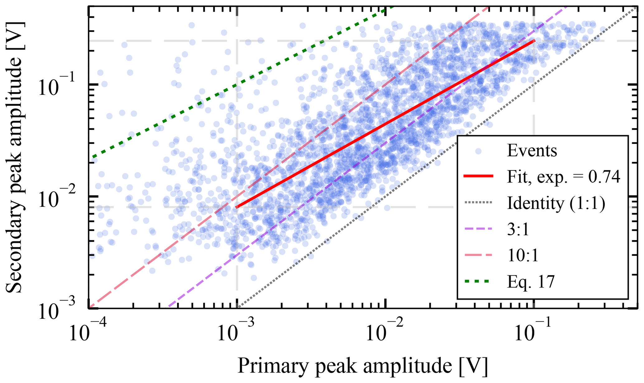
Figure 17 The estimate of the ratio $V_{\sec }/V_{\mathrm{pr}}$ for the process responsible for the secondary peaks. Each point corresponds to one impact in which a secondary peak was observed. The least-squares fit is shown, alongside 1:1, 3:1, and 10:1 ratio lines and Eq. (19).

The ion motion provides a good explanation for the delay of the secondary peak (see discussion in Sect. 5.1), yet the Pantellini et al. process in the present form does not explain the timescale of ≳100 µs over which the effect lasts. This is obviously too long for electron motion dynamics but in agreement with the ion motion timescales. In the original paper of Pantellini et al. (2012a), the authors describe how the photoelectron trajectories are temporarily altered due to the presence of a relatively weak electric field of the expanding plasma cloud. This alteration suppresses the photoelectron return current for a time, so that the affected electrons orbit around the influenced antenna's axis. In order to have a longer-lasting secondary peak, as we do, a sink for the excess photoelectrons is required, so that the photoelectrons are not recollected by the antenna on the electron motion timescale, which is what is suggested by Kellogg (2017). The claim that the electrons do not return to the antenna they were emitted from is supported by Zaslavsky et al. (2012), who reported the exponential decay profile of the pulses that were believed to be caused by the Pantellini et al. process. Since the ion cloud does not provide a field strong enough to liberate a significant portion of the bounded photoelectrons to reach infinity, the sink for the photoelectrons has to be present at around the antenna potential. The only suitable sink here is provided by the spacecraft body. Since the body potential is similar to the antenna potential, the affected electrons orbiting around the antenna axis are free to migrate along the antenna axis and can reach it rather easily. Moreover, due to the BIAS subsystem of RPW, the spacecraft body is usually on a somewhat higher potential, compared to the antenna potential (Maksimovic et al., 2020). Given all this, we believe that an important portion of the affected electrons is recollected by the spacecraft's body, so the secondary peak is therefore a result of a temporarily amplified current between the affected antenna and the body. A consequence of this is that each such antenna-emitted body-collected electron is counted twice in the affected monopole channel; hence the peak is enhanced further. Also, the body potential is changed, albeit by a difference smaller by the ratio of the antenna's and the body's capacitance, which then shows synchronously in all the channels – a phenomenon that is observed reasonably often.

6 Conclusions

We studied the charge generation electrical process upon the impact of a dust particle on the surface of Solar Orbiter, as recorded with RPW electrical antennas. We found double-peak dust impact signals in about 50 % the electrical waveforms containing dust impact signatures. To the best of our knowledge, this is the first time such double-peak impact signatures were systematically observed and analyzed.

Upon inspection of the primary peak, we conclude consistence with the state-of-the-art theory for body potential influence by the impact charge. Our analysis indicates a mean impact charge magnitude of 21 pC and a median impact charge magnitude of 8 mV. We find that the rise time of the primary peak is variable and consistent with the timescale of the photoelectron sheath shielding of the impact cloud. We find the decay time consistent with the timescale of the potential equalization due to ambient charge collection. We were able to explain the small observed asymmetry between the primary peaks recorded in individual channels with electrostatic influence of antennas, on top of an otherwise symmetric peak caused by the change in body potential.

The secondary peak is found to be highly variable and very asymmetric with respect to the three channels. A relatively long delay of ≈100–300 µs with respect to the primary peak suggests that the secondary peak's presence is linked to the impact cloud moving much closer to the antennas. This delay is consistent with an ion escape velocity of 10–20 km s⁻¹. We concluded that the observed amplitudes of the secondary peak are too strong for either impact charge collection by antennas or antennas being immersed in impact cloud potential, which clearly suggests the presence of an additional effect.

We found that the assumption that the channel maxima correspond to the impact charge leads to a systematic error. We believe that the primary peak is the better measure of the impact charge, compared to the global maximum of the channel, which is more likely influenced by the often-present secondary peak. It is therefore advisable to disregard the channel which shows the highest amplitude and to study the amplitudes of the primary peaks instead – the exact procedure used in present work is described in Appendix D.

Our semi-quantitative explanation of the secondary peak's appearance uses the photoelectron sheath perturbation effect, first described in Pantellini et al. (2012a). Furthermore, we hypothesize that the Pantellini et al. (2012a) effect might temporarily enhance the current between the antenna and the spacecraft body, as this would explain the longer-lasting nature of the secondary peaks. Importantly, the amplitudes of the secondary peaks are likely related to the impact location on the spacecraft and the delay between the primary and the secondary peak provides a measure of the location and of the ion expansion speed. This is worthy of future investigation and may prove useful for identification of the dust population, which the incident dust grain came from.

Appendix A: RPW measurement modes

Table A1 The relations between the channels in different measurement modes of RPW. For compactness, $V\mathrm{1};V\mathrm{2};V\mathrm{3}$ denote the voltages between the antenna $\mathrm{1};\mathrm{2};\mathrm{3}$ and the spacecraft body, respectively.

The Radio and Plasma Waves (RPW)electrical suite consists of three cylindrical antennas. There are three measurement modes: monopole (SE1), dipole (DIFF1), and mixed (XLD1). Whichever the mode RPW is in, it produces three channels of electrical data. See Table A1 for the modes' description and Souček et al. (2021) for much more comprehensive explanation.

Since the device spends by far the most time in XLD1 mode, it was chosen as the only mode of interest. Since the monopole data (SE1) are symmetric and the easiest to interpret, the XLD1 data are decomposed to SE1-like data for the analysis and visualization. The decomposition is performed as follows:

$$\begin{array}{}\text{(A1)}& {\displaystyle }\mathrm{V}\mathrm{1}=\mathrm{CH}\mathrm{3}-\mathrm{CH}\mathrm{2}\text{(A2)}& {\displaystyle }\mathrm{V}\mathrm{2}=\mathrm{CH}\mathrm{3}\text{(A3)}& {\displaystyle }\mathrm{V}\mathrm{3}=\mathrm{CH}\mathrm{3}-\mathrm{CH}\mathrm{2}-\mathrm{CH}\mathrm{1}.\end{array}$$

Though such decomposition provides the data user with the three reconstructed monopole channels, the user should be careful for two reasons: first, the saturation level is not clearly defined, as a difference between two saturated signals might not have been saturated otherwise, and second, the transfer function of a dipole is different to the transfer function of a monopole; hence the signal might be distorted, especially the components near the threshold frequencies. These limitations do not prohibit the analysis as described in the present publication.

Appendix B: Raw data filtering

The voltage data WAVEFORM_DATA_VOLTAGE of _rpw-tds-surv-tswf-e_ are used and are only calibrated by a constant, rather than the full empirical transfer function. Since the data show a high-frequency artificial modulation at ≈80 and ≈110 kHz, the data are filtered with the Butterworth low-pass filter of 32nd order at f_lo=70 kHz, which leaves us with the temporal resolution of τ_min≈14 µs.

According to the system's response function as measured by the RPW's engineering team, there is a significant low-frequency distortion in the <2 kHz region. There is also a minor high-frequency distortion in the f>50 kHz region, which we decided to not correct for, as its impact is very limited. The low-frequency part is corrected using Laplace-domain correction, as the very limited window length of 62 ms introduces other artifacts should the Fourier-domain correction be used. The first-order filter with the critical frequency of f_hi=370 Hz (see Eq. B1) was found to be the best fit according to the response spectrum; see Fig. B1.

$$\begin{array}{}\text{(B1)}& v_{\mathrm{corr}}\left(t\right)=v_{\mathrm{orig}}\left(t\right)+\mathrm{2}\mathit{\pi }{f}_{\mathrm{hi}}\underset{\mathrm{0}}{\overset{t}{\int }}v\left(\mathit{\tau }\right)\mathrm{d}\mathit{\tau }\end{array}$$

As a result, the corrected signal stays well corrected in the range of 500 Hz $<f<\mathrm{70}$ kHz. We note that higher-order effects might be present as well, which, along with the error we introduce when dividing a small value by another, place a limit on the reliability of the low frequencies below 500 Hz. For the spectra before and after the corrections, see Fig. B2. For the signal before and after the corrections applied, see Fig. B3; pay attention to the overshoot attenuated and the secondary overshoot eliminated.

Figure B1 The RPW's response function and the Laplace-domain correction.

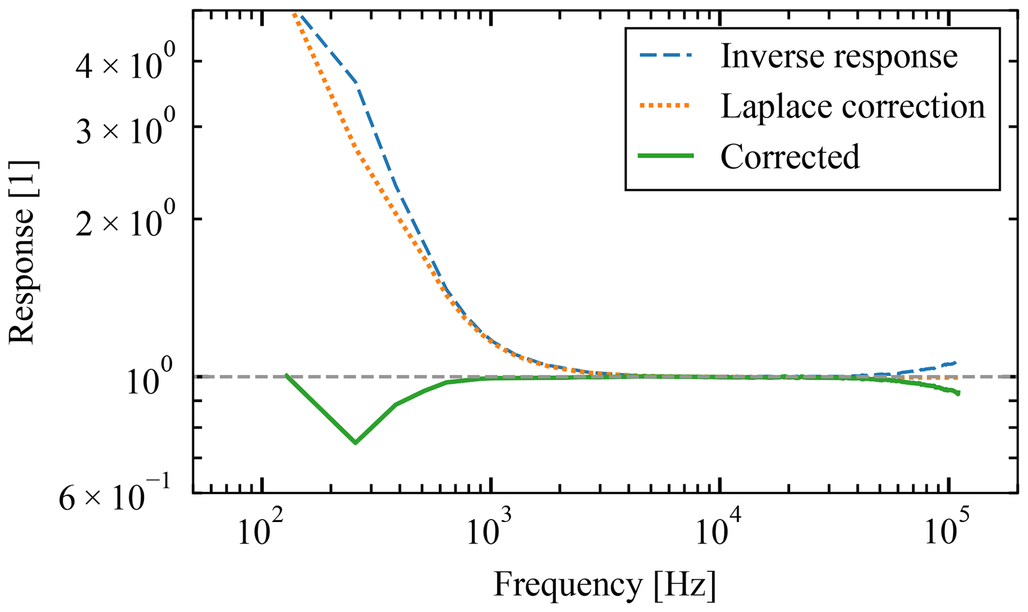
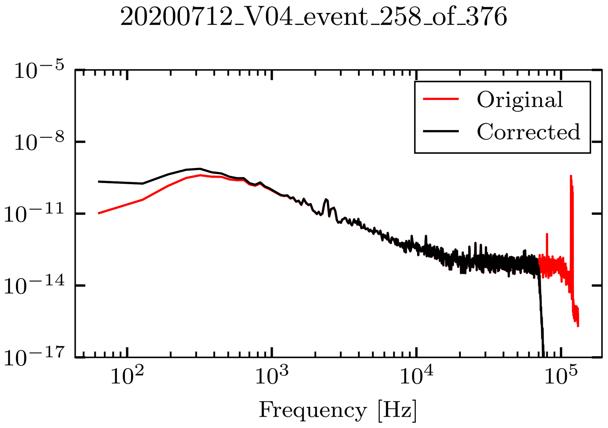
Figure B2 The spectrum of an electrical signal, before the low-pass and the Laplace corrections as well as after. We note that Laplace correction changes the signal on the low-frequency end only, while low-pass filter changes the high-frequency end.

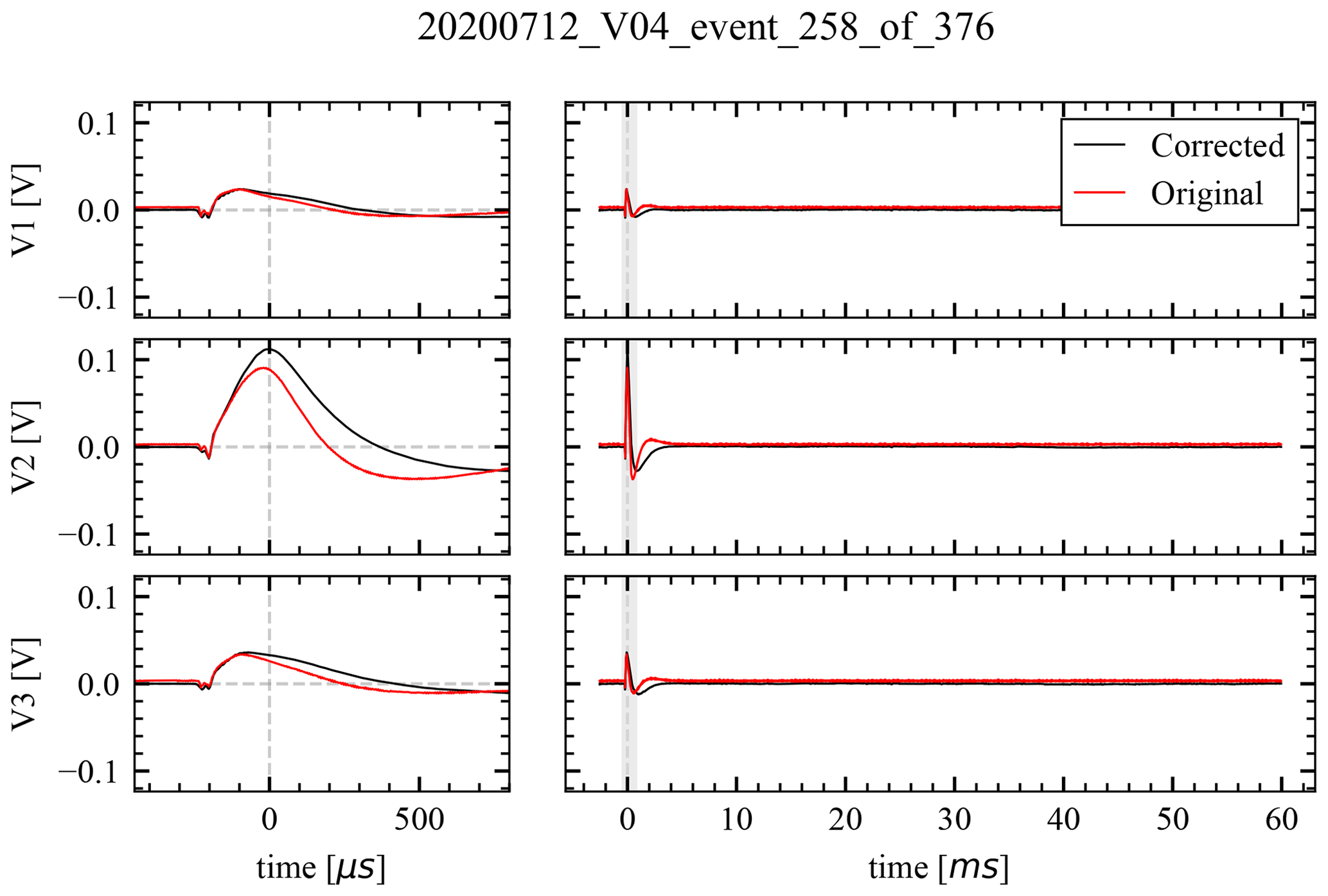
Figure B3 The waveform time series of an electrical signal, where the red line shows voltage time series before the low pass and the Laplace corrections, while the black line shows the same after the two corrections. The left-hand side shows detail of the shaded portion of the right-hand side, which in turn shows the whole recording of 62 ms.

Appendix C: Ternary plot for primary and secondary peaks

The ternary plot in Fig. 2 shows a data point for every event, with the amplitudes based on the channel global maximum. In sections starting with Sect. 2 we treat the waveforms as containing two major peaks (called primary and secondary), while the latter is not always present. Since we argue that the ternary plot (Fig. 2) shows this indirectly, it makes sense to redo the ternary plot for the XLD1 events that do and do not contain secondary peaks respectively; see Fig. C1. It is clear that the primary peaks are much more consistent across the channels, compared to the cases when secondary peaks are added.

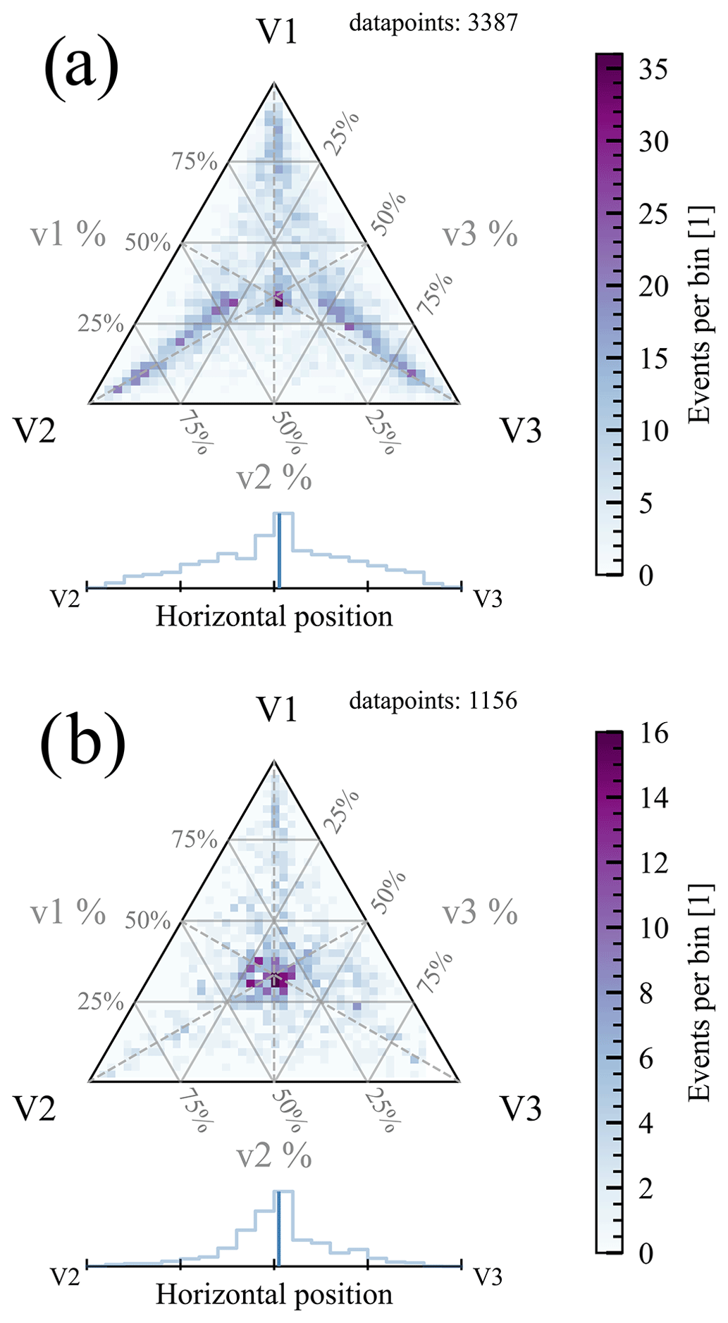
Figure C1 Ternary plot for the global maxima of the three monopole channels, one point for each XLD1 event. (a) The impacts that do show at a secondary peak in at least one channel and (b) the impacts that do not show any secondary peak in either channel.

Appendix D: Feature extraction

The signals of interest (as defined in Sect. 2.3) were analyzed as follows:

1. A positive primary peak is assumed to be present in each channel, and it is assumed to be of the same amplitude V_body in all the channels. The reason is that it is a rather typical case that the primary peak is obscured by a much larger peak in a close succession in at least one of the channels. Therefore, the amplitude of the primary peak is established as the mean of the amplitude of the weaker two, with the reference zero as the mean of the non-affected background signal shortly preceding the impact. The temporal location of the peak is first found approximately, using a minimum of the second derivative near the global signal maximum, and then precisely, using a local maximum in the correlation of the signal and a one-sided parabola, which works for both distinct peaks and inflection points. The pre-spike and body locations are identified as demonstrated in Fig. D1.

2. The rise time of the primary peak is evaluated as the time to get from 43 % to 80 % of the maximum amplitude, assuming zero on the preceding background level. This range (37 %) corresponds to $\mathrm{1}/e$ of the maximum and is chosen so that neither the flat nature of the primary peaks nor the background noise influences the estimate.

3. A secondary positive peak may or may not be present in each of the channels separately. First, primary peak is subtracted from the data in the form of asymmetric Gaussian peak with the rise time ${\mathit{\tau }}_{\mathrm{rise}}^{\mathrm{body}}$ given by the data and the decay time ${\mathit{\tau }}_{\mathrm{decay}}^{\mathrm{body}}$ assumed to be equal to $\mathrm{3}{\mathit{\tau }}_{\mathrm{rise}}^{\mathrm{body}}$, as that is found to be a good approximation in cases where no secondary peak is present. Second, the secondary peak is considered present if the signal after the subtraction of the primary peak shows a maximum of amplitude of at least 75 % of the primary peak. Then amplitudes of the present secondary peaks (after primary peak subtraction) are measured. See this step shown in Fig. D2.

4. The decay time of the primary peak is only evaluated on the channel with the lowest global maximum and is done so as the time in takes the signal to decay from 100 % to 63 %, that is $\mathrm{1}/e$. Here we evaluate the decay time closer to the maximum as the undershoot effects and the possible secondary peak influence the result much more than the flat nature of the primary peak or the noise.

5. A negative pre-peak may or may not be present and is assumed to be of the same amplitude in all three channels. The presence is decided by a 3 σ criterion with regard to the noise. If the peak is found present, the amplitude of the primary peak is corrected by this value in the last step.

Given that in most cases the primary peak is not the channel maximum, careful analysis is advised, as opposed to the assumption that the channel maximum is proportional to the amount of generated charge. However, the secondary peak is only present in one of the channels, therefore assuming that the lowest of the three maxima to be proportional to the amount of generated charge leads to a systematic error that is a lot lower and is advised if a more careful approach is not an option.

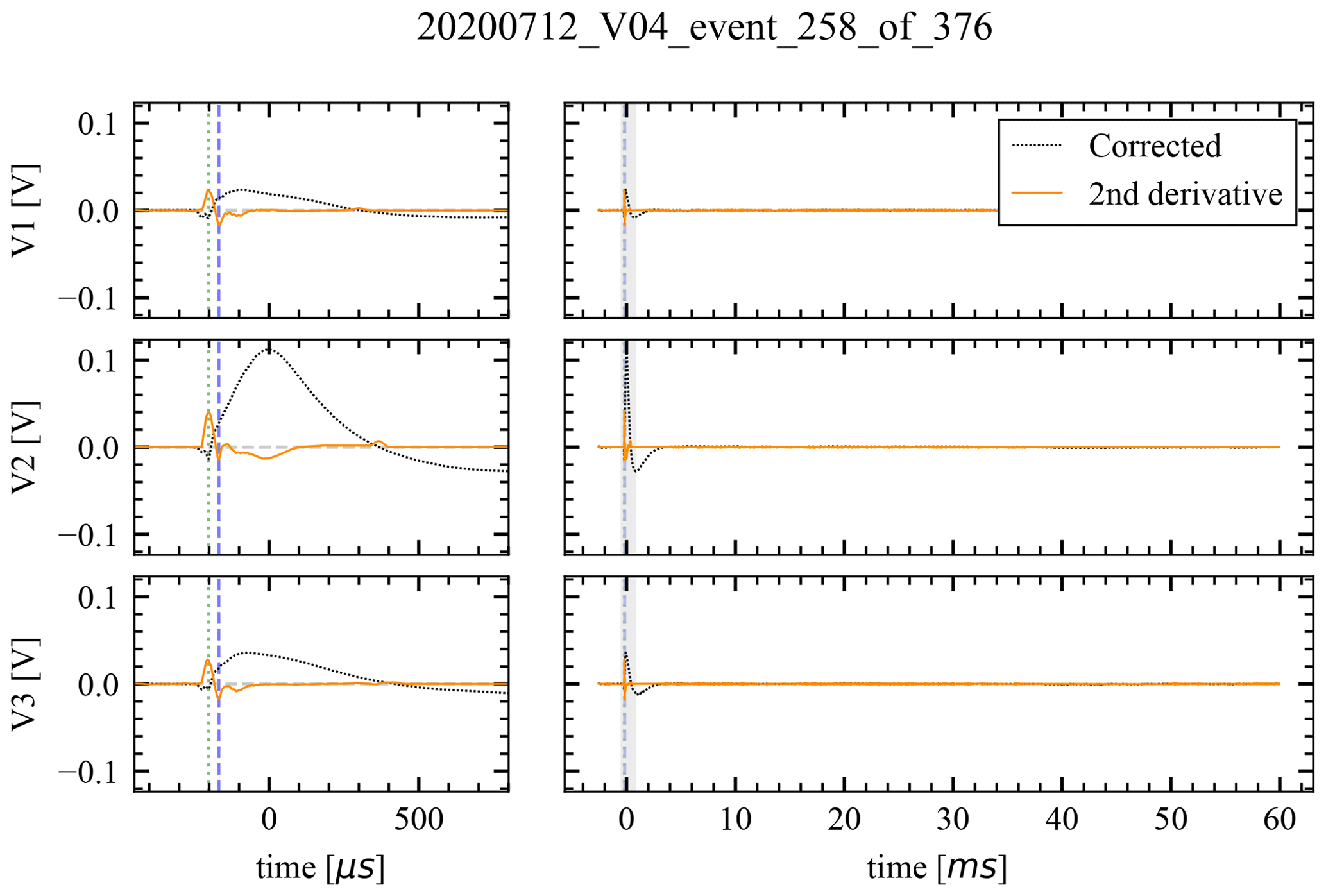
Figure D1 The waveform time series of an electrical signal. The dotted black line shows the voltage signal after the spectral corrections, while the yellow line shows the second derivative. The vertical dashed green and blue lines show the locations of the negative pre-spike and the primary peak, respectively. The left-hand side shows detail of the shaded portion of the right-hand side, which in turn shows the whole recording of 62 ms.

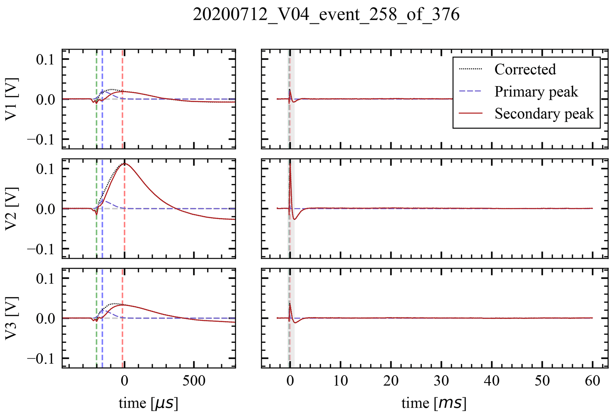
Figure D2 The waveform time series of an electrical signal. The dotted black line shows the voltage signal after the spectral corrections, while the dashed blue line shows the approximated primary peak. The primary peak is subtracted from the measured signal, and the residual is plotted as the red line. The vertical dashed green, blue, and red lines show the locations of the negative pre-spike, the primary peak, and the secondary peaks respectively. The left-hand side shows detail of the shaded portion of the right-hand side, which in turn shows the whole recording of 62 ms.

Appendix E: Primary peaks' amplitude distribution

In Sect. 4.1 we report on the amplitudes of the primary peaks that are connected to the amount of charge liberated at dust impacts. See Fig. E1 for the normalized histogram of the amplitudes. We note that no signals with global maxima over 300 mV are included, which also disqualifies the signals with V_body<300 mV provided that the secondary peak is over the threshold – leading to underestimation of high amplitude (≳ 100 mV) counts. Also, given the secondary peak is often of the highest amplitude present, recognition of low-amplitude primary peaks is conditioned by the presence of a secondary peak. Therefore, the presence of small primary peaks (≲ 10 mV) is underestimated by a factor that is hard to evaluate. The former bias is more apparent in the black line of Fig. E1, while the latter is more apparent in the light-blue line of the same figure.

We note that, contrary to the distribution of global maxima of the signal on an arbitrary monopole (Zaslavsky et al., 2021), the distribution of the primary peaks' amplitudes does not resemble a power law. This is not a basis to claim that the power law is not present in the distribution of amplitudes, or by extension masses, as there is selection bias present, as was mentioned previously.

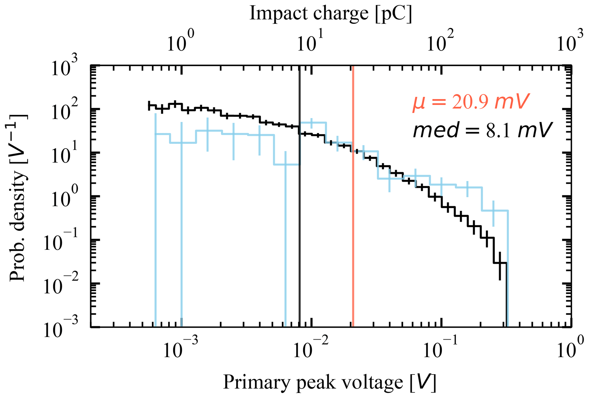
Figure E1 Histogram (normalized) of the primary peak amplitudes of all the signals in black; the mean and median are also shown. A separate normalized histogram of only those hits that do not show a secondary peak in any channel is shown in light blue. The vertical error bars represent the 90 % confidence intervals obtained by bootstrapping. The conversion from the peak voltage to the impact charge is $V/Q={\mathrm{10}}^{\mathrm{9}}V/C$.

Appendix F: Primary peak asymmetry – the model for antennas' response to a point charge

The model assumes antennas in a plane that are made of thin wire and are 6.5 m long. A response of these antennas to a test charge is calculated, alongside the calculation of the spacecraft's body response to the same charge as by Eq. (2). In order to produce samples of signal responses, the model samples charge locations (impact spots) from a plane parallel with the antenna plane and 1 m in front of the antenna plane, in the rectangle of 2.4 m by 3.1 m, which approximately coincides with the size and the relative location of the Solar Orbiter's heat shield; see Fig. F1. The potential of an antenna is integrated numerically as the average field along the antenna, according to equations in Sect. 3.3.1. The value of λ_D is assumed infinite; hence Eq. (5) is simplified to

$$\begin{array}{}\text{(F1)}& \mathrm{\Phi }={\displaystyle \frac{Q}{\mathrm{4}\mathit{\pi }\mathit{ϵ}}}{\displaystyle \frac{\mathrm{1}}{|\mathit{x}-{\mathit{x}}_{\mathit{q}}|}}.\end{array}$$

The ch1, ch2, and ch3 are calculated as the sum of the respective antenna's response with the spacecraft body's response, since the body detects negative, while antennas detect positive charge. We note that a simplification is present: the maxima of the peak of the body response and the peak of the antenna response are typically not synchronous, yet we treat them as such in order to evaluate the ratios of the channel maxima shown in Fig. 6.

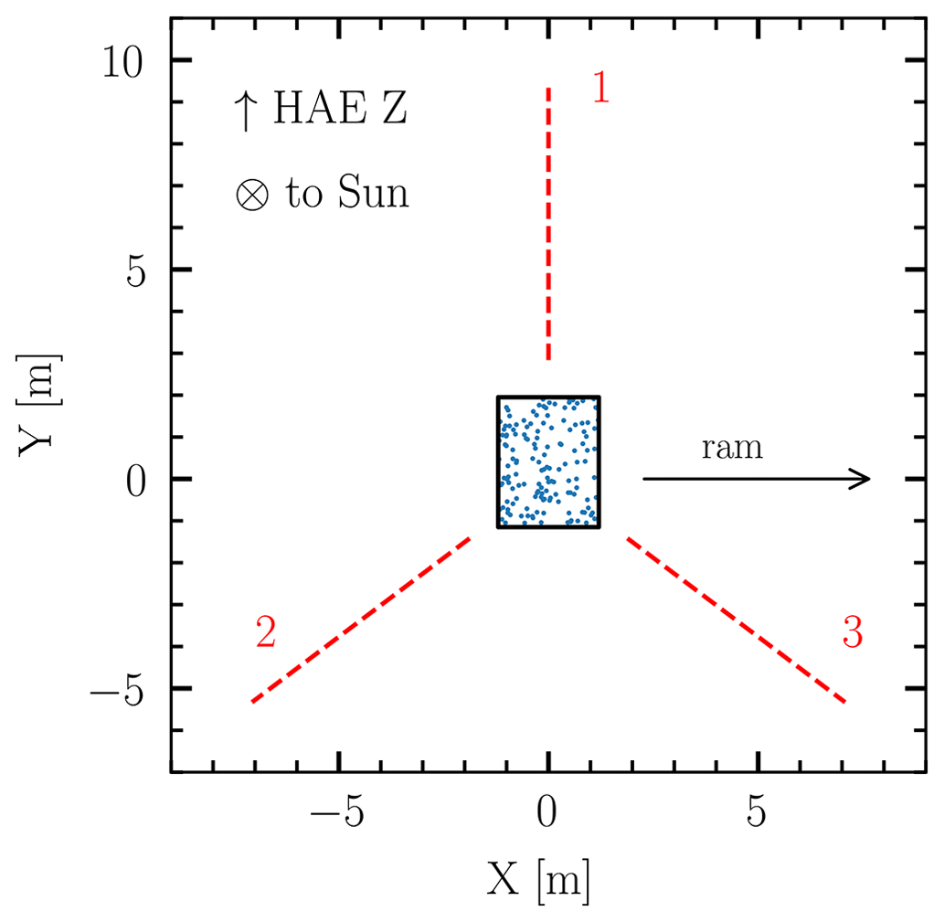
Figure F1 The Solar Orbiter's heat shield (black rectangle) and the RPW antennas (dashed red) viewed from behind, as used for the purpose of the antennas' response to a point charge modeling – sampling illustrated.

Appendix G: Impact cloud potential and photoelectron temperature

The photoelectrons near the illuminated areas of the spacecraft provide a relatively dense ($\approx {\mathrm{10}}^{\mathrm{8}}{\mathrm{m}}^{-\mathrm{3}}=\mathrm{100}$ cm⁻³) region of free negative charges (Meyer-Vernet et al., 2017), with the corresponding photoelectron Debye length of ${\mathit{\lambda }}_{ph}\approx \mathrm{0.29}-\mathrm{0.98}$ m at the heliocentric distance of $R=\mathrm{0.25}-\mathrm{1}$ AU (Guillemant et al., 2013). The photoelectron sheath is therefore effective at screening the escaping positive impact cloud from the spacecraft body after it has passed sufficiently far from the body, which is indeed the process that seems to control the rise time of the primary peak; see Sect. 4.2 and Meyer-Vernet et al. (2017). However, the cloud escapes the vicinity of the spacecraft, and it is not straightforward to determine whether it will do so neutralized by the photoelectrons it was exposed to or not. A possible estimate is done by comparing the typical photoelectron energy with the potential barrier the predominantly positive ion cloud poses for them. Should the photoelectrons be relatively cold, compared to the depth of the potential hole of the cloud, they are likely to be captured and hence to neutralize the cloud. Should the photoelectrons be much more energetic than the ion cloud potential hole, they are likely to screen only and to not be bounded by the cloud, therefore not neutralizing it.

An order-of-magnitude photoelectron energy may be done by comparing the incident UV photon energy (≈10 eV) and the spacecraft's surface material work function (≈4 eV), yielding the typical photoelectron energy of 6 eV near the surface. Guillemant et al. (2013) used the mean photoelectron energy at emission of 3 eV and 10 eV in their numerical estimates of the spacecraft charging. The kinetic energy of an electron at its maximum extent from the antenna is very low. Let our order-of-magnitude estimate be T_ph=3 eV.

For an order-of-magnitude estimate of the ion cloud's potential, let us assume spherical expansion of the cloud and a uniform distribution of the charge within the cloud. Assuming the most extreme case, that is the cloud made of cations only, the mean charge of the cloud is Q≈21 pC (see Sect. 4.1). Then, the potential Φ within the cloud of radius R at the distance from the center of r is readily obtained as

$$\begin{array}{}\text{(G1)}& \mathrm{\Phi }={\displaystyle \frac{\mathrm{1}}{\mathrm{4}\mathit{\pi }{\mathit{ϵ}}_{\mathrm{0}}}}{\displaystyle \frac{r^{\mathrm{2}}Q}{R^{\mathrm{3}}}}.\end{array}$$

The maximum potential is present at the edge of the cloud (r=R); that is

$$\begin{array}{}\text{(G2)}& {\mathrm{\Phi }}_{\max }={\displaystyle \frac{\mathrm{1}}{\mathrm{4}\mathit{\pi }{\mathit{ϵ}}_{\mathrm{0}}}}{\displaystyle \frac{Q}{R}},\end{array}$$

which numerically is

$$\begin{array}{}\text{(G3)}& {\mathrm{\Phi }}_{\max }\approx {\displaystyle \frac{\mathrm{0.2}\mathrm{Vm}}{R}},\end{array}$$

or

$$\begin{array}{}\text{(G4)}& {\displaystyle }{\mathrm{\Phi }}_{\max }(R=\mathrm{10}\mathrm{cm})\approx \mathrm{2}\mathrm{V};\text{(G5)}& {\displaystyle }{\mathrm{\Phi }}_{\max }(R=\mathrm{1}\mathrm{m})\approx \mathrm{0.2}\mathrm{V}.\end{array}$$

We see that the simple order-of-magnitude estimate shows that the potential within the impact cloud drops below the photoelectron energy well within 10 cm of expansion, suggesting that one may neglect it in calculating the photoelectron current collected by the cloud.