the Creative Commons Attribution 4.0 License.
the Creative Commons Attribution 4.0 License.
 | 29 May 2024
Application of generalized aurora computed tomography to the EISCAT_3D project
Yoshimasa Tanaka
Yasunobu Ogawa
Akira Kadokura
Takehiko Aso
Björn Gustavsson
Urban Brändström
Tima Sergienko
Genta Ueno
Satoko Saita
EISCAT_3D is a project to build a multi-site phased-array incoherent scatter radar system in northern Fenno-Scandinavia. We demonstrate via numerical simulation how useful monochromatic images taken by a multi-point imager network are for auroral research in the EISCAT_3D project. We apply the generalized aurora computed tomography (G-ACT) method to modelled observational data from real instruments, such as the Auroral Large Imaging System (ALIS) and the EISCAT_3D radar. G-ACT is a method for reconstructing the three-dimensional (3D) distribution of auroral emissions and ionospheric electron density (corresponding to the horizontal two-dimensional (2D) distribution of energy spectra of precipitating electrons) from multi-instrument data. It is assumed that the EISCAT_3D radar scans an area of 0.8° in geographic latitude and 3° in longitude at an altitude of 130 km with 10 × 10 beams from the radar core site at Skibotn (69.35° N, 20.37° E). Two neighboring discrete arcs are assumed to appear in the observation region of the EISCAT_3D radar. The reconstruction results from G-ACT are compared with those from the normal ACT as well as the ionospheric electron density from the radar. It is found that G-ACT can interpolate the ionospheric electron density at a much higher spatial resolution than that observed by the EISCAT_3D radar. Furthermore, the multiple arcs reconstructed by G-ACT are more precise than those by ACT. In particular, underestimation of the ionospheric electron density and precipitating electrons' energy fluxes inside the arcs is significantly improved by G-ACT including the EISCAT_3D data. Even when the ACT reconstruction is difficult due to the unsuitable locations of the imager sites relative to the discrete arcs and/or a small number of available images, G-ACT allows us to obtain better reconstruction results.
- Article
(11960 KB) - Full-text XML
- BibTeX
- EndNote


EISCAT_3D is a multi-point phased array incoherent scattering radar system under construction in northern Fenno-Scandinavia as of November 2023 and is expected to be operational in winter 2023. The EISCAT_3D radar will be able to measure the three-dimensional (3D) distribution of ionospheric parameters, such as the electron density, electron temperature, ion temperature, and ion Doppler velocity, at a resolution that is more than 10 times higher than that of the existing EISCAT radar. Thus, it is expected to provide new insights into various science topics pertaining to auroral physics, ionospheric physics, magnetosphere–ionosphere coupling, and so on (McCrea et al., 2015; Wannberg et al., 2010).
The height distribution of the ionospheric electron density in the auroral region, which is related to the energy distribution of auroral precipitating electrons, is essential for clarifying if the precipitating electrons experienced acceleration and to determine their place of origin. In addition, we can estimate the ionospheric conductivity from the electron density by using empirical models (e.g., the Mass Spectrometer and Incoherent Scatter (MSIS) atmosphere model and the International Geomagnetic Reference Field (IGRF) model; Hedin, 1991; Alken et al., 2021). It is well known that the spatial distribution of ionospheric conductivity plays an essential role in the magnetosphere–ionosphere coupling process (e.g., Ellis and Southwood, 1983; Glaßmeier, 1984; Itonaga and Kitamura, 1988). It may be possible to deduce a 3D current system from the ionospheric conductivity distribution by using magnetic field data from a ground-based magnetometer array and/or ionospheric electric field data from radars (Kamide et al., 1981; Vanhamäki and Amm, 2007).
On the other hand, it is useful to utilize optical imaging observations to study auroral dynamics. Radars generally have a high range resolution; however, scanning a particular area with multiple beams is time-consuming. In contrast, an optical imager has a high angular resolution. It can measure angular distributions at a higher temporal resolution than a radar, even though it can detect only the integrated luminosity along the line of sight. In other words, the radar and optical imager are complementary. Therefore, it is essential to use image data with radar data effectively. Figure 1 shows a schematic illustration of the relationship between the radar and imager observations.
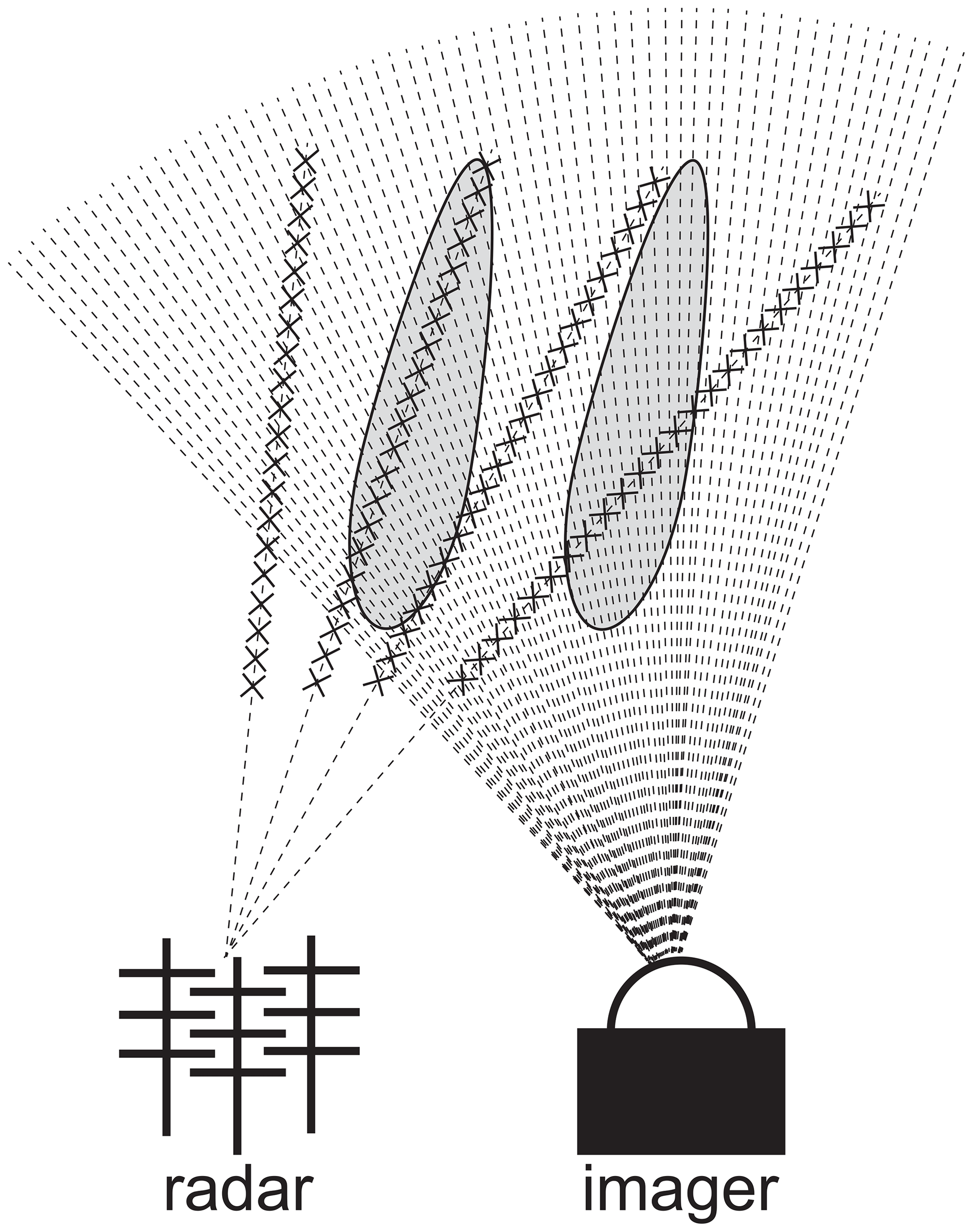
Figure 1Schematic illustration of the relationship between the radar and optical imager observations.
There are some ground-based imager networks in northern Fenno-Scandinavia, e.g., the Aurora Large Imaging System (ALIS) (Brändström, 2003), the all-sky cameras in the Magnetometers – Ionospheric Radars – All-sky Cameras Large Experiment (MIRACLE) (Syrjäsuo, 2001), and Watec Monochromatic Imager (WMI) (Ogawa et al., 2020). In particular, the ALIS was designed to obtain the 3D distribution of the optical emissions in the mesosphere, thermosphere, and ionosphere, and was recently developed into ALIS_4D (https://alis4d.irf.se/, last access: 5 May 2024). By applying the auroral computed tomography (ACT) technique to the monochromatic images taken at some ALIS stations, it is possible to retrieve the 3D distribution of auroras that have a horizontal scale of several tens to hundreds of kilometers (Aso et al., 1998; Gustavsson, 1998; Gustavsson et al., 2001; Simon Wedlund et al., 2013). Conversely, the inverse problem of ACT is ill-posed and ill-conditioned, because the optical image data correspond to the emission intensity integrated along the line of sight and only a few images are usually available. Thus, assumptions need to be made to solve the inverse problem, which often makes it somewhat difficult to interpret the results of the data analysis from a physical point of view.
Aso et al. (2008) and Tanaka et al. (2011) have extended ACT to the generalized ACT (G-ACT). This method can reconstruct the spatial and energy distributions of auroral precipitating electrons by using multi-instrument data, such as the ionospheric electron density from an incoherent scatter radar, the cosmic noise absorption (CNA) from an imaging riometer, and optical monochromatic images. Tanaka et al. (2011) demonstrated via numerical simulation that the reconstruction from only auroral images can be improved by G-ACT by using the height profile of the electron density from the EISCAT radar.
In the current study, we investigated how effective the combination of the EISCAT_3D radar and the monochromatic imager network is for auroral research by conducting a simulation. We apply the G-ACT method to the modelled observational data, i.e., electron density from the EISCAT_3D radar and the multiple monochromatic images from the ALIS, and compare the reconstruction results with those obtained by the normal ACT and the radar's electron density data. We selected the ALIS (not ALIS_4D) as the monochromatic imager network for this simulation study, because the monochromatic images from the ALIS can be used for both the normal ACT analysis and the G-ACT analysis. It is possible to compare the auroral 3D distributions reconstructed by the two methods in the same region because one of the ALIS stations is located in Skibotn (69.35° N, 20.37° E), Norway, which is the core site of the EISCAT_3D radar, and the field of view (FOV) of the ALIS imagers covers the radar observation region.
2.1 Observatories and instruments
Figure 2 shows the locations of the stations used in this simulation study and each instrument's fields of view (FOVs) at an altitude of 130 km. Blue quadrangles and red crosses correspond to the FOVs of the ALIS imagers and the beam position of the EISCAT_3D radar, respectively. The core site of the EISCAT_3D radar is located at Skibotn, Norway.
It was assumed that the EISCAT_3D radar scanned an area of geographic latitude from 68.6 to 69.4° N and longitude from 18.767 to 21.767° E at an altitude of 130 km with 10 × 10 beams, which corresponds to a spatial resolution of 0.08° (about 8.9 km) in latitude and 0.3° (about 12 km) in longitude. It was also assumed that the electron density was detected at altitudes between 90 and 170 km. The dot-dash line indicates the region where the reconstruction results were evaluated, which is the same as the dot-dash line in Fig. 3a.
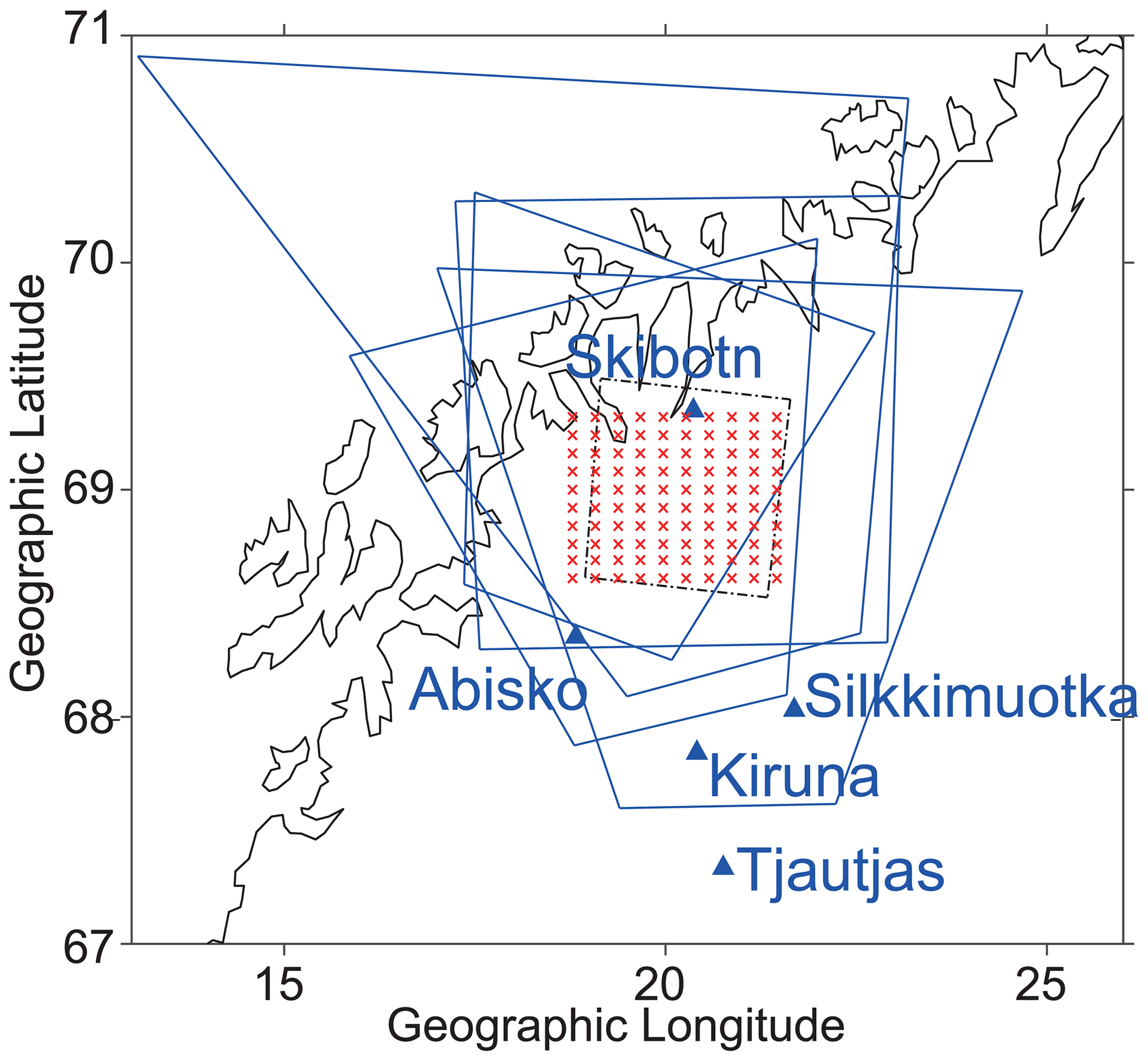
Figure 2Locations of the stations used in this study and the fields of view (FOVs) of the ALIS imagers and EISCAT_3D radar at an altitude of 130 km. It was assumed that the viewing direction of the imagers was set to the south of Skibotn and the radar scanned an area of geographic latitude from 68.6 to 69.4° N and longitude from 18.767 to 21.767° E with 10 × 10 beams.
Each ALIS station has a sensitive high-resolution (1024 × 1024 pixels) unintensified monochromatic CCD imager with a six-position filter wheel for narrowband interference filters (427.8, 557.7, 630.0, and 844.6 nm) (Brändström, 2003). The FOV of each imager is about 50 to 90°. It was assumed that the viewing direction was set to the south of Skibotn and the filter was fixed to the N first negative band (427.8 nm) for all stations. We postulated that the image size was reduced to 256 × 256 pixels after 4 × 4 pixel binning.
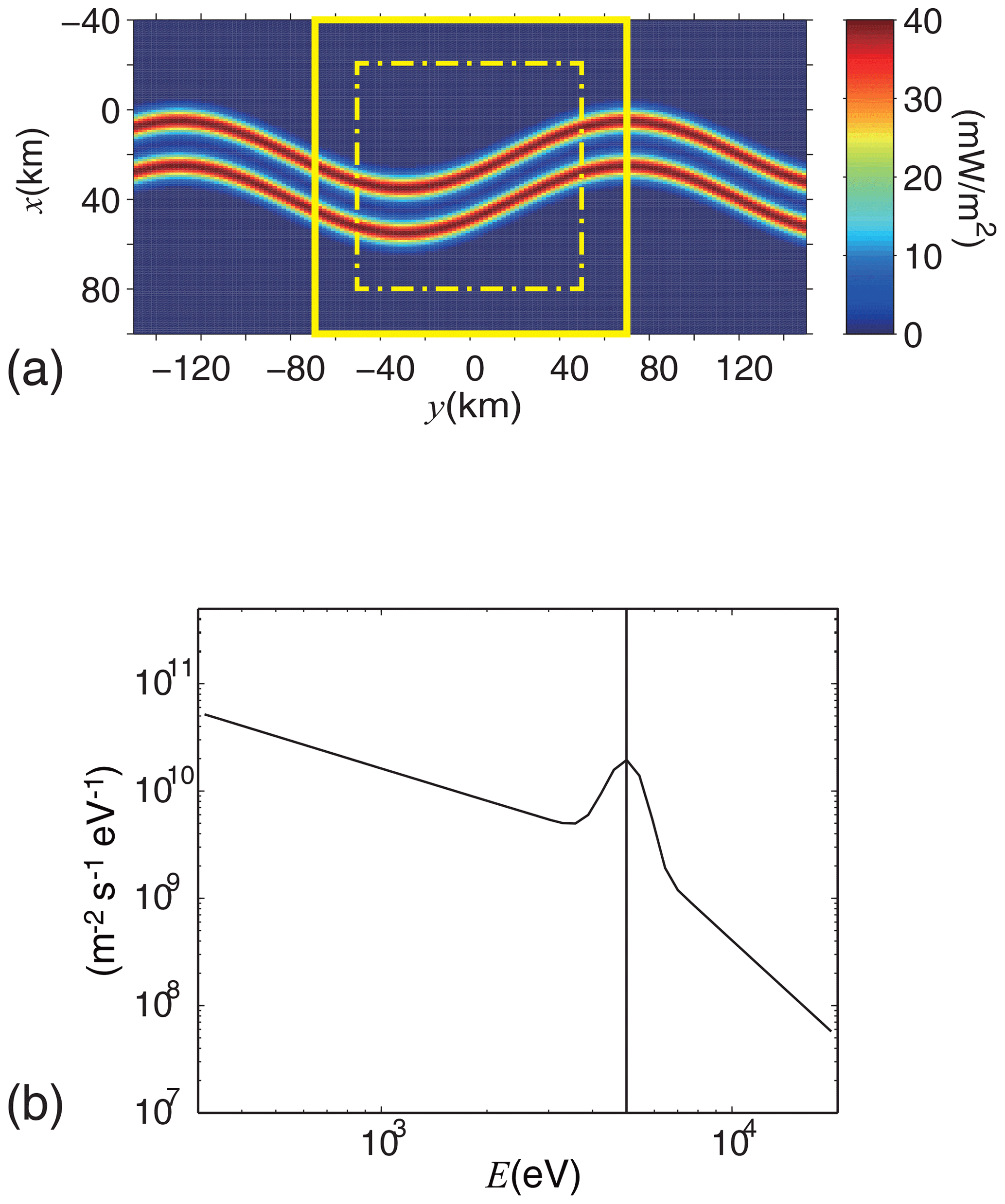
Figure 3(a) Horizontal distribution of the total energy flux (Q0) of the incident auroral electrons. The top and right correspond to the geomagnetic northward and geomagnetic eastward directions, respectively. The thick line and dot-dash line indicate the region used for the inverse analysis and the region where the reconstruction results were evaluated, respectively. (b) Energy distribution of the incident electrons at the peak location of the discrete arcs.
2.2 Distribution of incident auroral electrons
Figure 3a indicates the horizontal distribution of the total energy flux (Q0) of the auroral precipitating electrons that was assumed for the forward analysis. It was also assumed that two neighboring discrete arcs appeared over the southern sky of Skibotn. In this simulation, an oblique coordinate system was adopted with an origin at Skibotn, with the x axis pointing in the geomagnetic southward direction, the y axis pointing in the eastward direction, and the z axis anti-parallel to the geomagnetic field (cf., Fig. 2 of Tanaka et al., 2011). The inclination and declination angles of the geomagnetic field were 78 and 6°, respectively. The calculation ranges were −40 to 100 km, −150 to 150 km, and 90 to 190 km for the x, y, and z directions, respectively. The spatial mesh sizes (Δx, Δy, Δz) were 1, 2, and 2 km for the x, y, and z directions, respectively. The discrete arcs were assumed to have a sinusoidal shape in the y direction and a Gaussian shape in the x direction. The distance between the two arcs was 20 km. The area surrounded by a thick line is the reconstruction region used for the inverse analysis in Sect. 3. The dot-dash line indicates the region where the reconstruction results are evaluated in Sect. 4.
Figure 3b shows the energy distribution of the differential number flux of the precipitating electrons at the peak location of the arcs. The energy spectrum is represented by the sum of the Gaussian distribution () and two power-law distributions for the low-energy tail (, E≤E0) and high-energy tail (, E≥E0), which has been introduced by Strickland et al. (1993) as a typical spectrum of discrete auroras. E0, W, a, and b were set to 5 keV, 0.15×E0, 1.0, and 3.0, respectively, for the entire simulation region. The energy range for the calculation was between 0.3 and 20 keV and divided logarithmically into 50 intervals.
Since the main purpose of this paper is to compare the results from the two analysis methods, ACT and G-ACT, we assumed a rough but typical auroral shape, size, and energy distribution. Actual auroras have a variety of shapes, including multiple arcs, structured shapes, patchy shapes, and very thin arcs less than 100 m thick. However, it is difficult to examine such a large number of auroral types in this paper due to a lack of space. If one wants to evaluate the accuracy of the tomographic analysis results for real auroras, simulations should be performed using modelled auroras that resemble them (e.g., Fukizawa et al., 2022).
2.3 Calculation of modelled data set
The formulation of our method is based on that used by Janhunen (2001). The forward problem was solved by using the distribution of the incident electrons described in Sect. 2.2. The height profile of volume emission rate along the field line at a certain horizontal coordinate (x1, y1) is calculated by
where is the energy distribution of differential number flux of incident electrons at the top of the ionosphere (x1, y1, zmax), and m1 is a matrix operator for calculating from . We adopted Rees' model (Rees, 1989) to obtain the energy deposition rate to the atmosphere from the differential flux and the method proposed by Sergienko and Ivanov (1993) to calculate the 427.8 nm volume emission rate from the energy deposition rate. The elements of m1 are a function of the atmospheric parameters, which were calculated by using the MSIS-90 atmosphere model (Hedin, 1991). The derivation of m1 is described in detail in the Appendix of Tanaka et al. (2011).
Assuming that m1 is independent of x and y, Eq. (1) can be expanded in the x and y directions as follows:
In Eq. (3), f is a function of x, y, and E and has a length of , and L is a function of x, y, and z and has a length of . M1 is a large sparse matrix whose size is m×n.
In a similar manner to L, a square of ionospheric electron density generated by the incident electrons is given by
where
M2 has the same size as M1. In Eq. (5), the electron density measured by the EISCAT_3D radar was assumed to be caused by the auroral precipitation only. For the derivation of m2, we assumed that the ionospheric electron density is quasi-steady-state and the ionization loss in the E-layer is dominated by the recombination process. Again, refer to the Appendix of Tanaka et al. (2011) for more details.
A gray level gi at a pixel i in the auroral image is approximated by a linear integration along a line of sight, as shown below:
where r, θ, and φ are polar coordinates whose origin is located at the center of the camera lens, and cg(θ,φ) is a sensitivity and vignetting factor. Equation (6) can be represented by
where g is a gray-level vector which has lg elements, and P1 is a lg× m matrix used to calculate g by integrating L along the line of sight.
The square of electron density observed by the EISCAT_3D radar d is expressed by the matrix expression:
where P2 is a ld× m matrix that extracts data in the voxels corresponding to the radar observation locations from .
We added the noise to d and g and finally obtained modelled data, and . Gaussian noise with a standard deviation of 5 % of the electron density was added to the electron density data. The offset of 300 R was added to the gray level data and then Gaussian noise with a standard deviation of was added. Figure 4a and b show the modelled ionospheric electron density that should be obtained by the EISCAT_3D radar and the modelled auroral images at five ALIS stations.
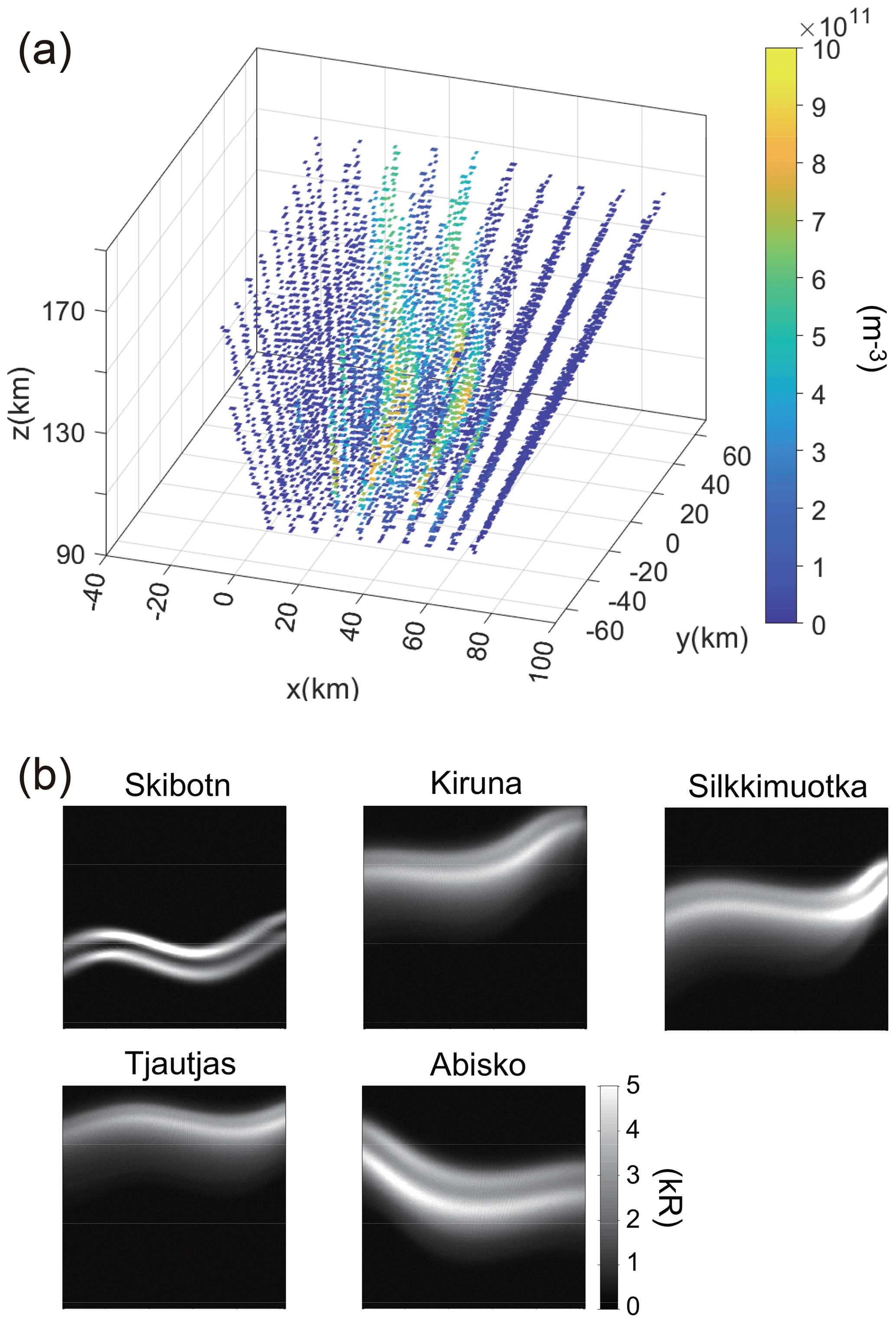
Figure 4(a) Modelled ionospheric electron density data obtained by the EISCAT_3D radar. (b) Modelled auroral images taken at five ALIS stations. Top and right of the images correspond to the northward and westward directions, respectively.
Our inverse analysis method is based on the Bayesian model. According to Bayes' theorem, the probability that model f is true after data were observed, i.e., the posterior probability ), is expressed by
where ) is the likelihood, which is the probability of observing data given model f; P(f) is the prior probability of model f; and ) is the marginal probability of . In this study, P(f) and ) are given by
where σ2 is the variance of ∇2f, where is the inverse covariance matrix, and where j means the kind of data. It was assumed that the modelled data are independent from each other, so has zero off-diagonal elements and the inverse of the variance of in the diagonal elements. corresponds to the modelled data and for j=1 and 2, respectively, and they include the noise. bj(f) corresponds to g and d in Eqs. (7) and (8). Equation (10) indicates the smoothness constraint on f with respect to x, y, and E. In Eq. (11), it was assumed that the modelled data has Gaussian errors. By substituting Eqs. (10) and (11) into Eq. (9), ) is given by
where wj is a hyper-parameter, which is a constant corresponding to the weighting factor for each instrument data.
Maximization of the posterior probability is equivalent to minimization of the function inside the curly brackets of Eq. (12), which is given by
Here, we define as follows;
Then, Eq. (13) is given by
Here, we change the variables by letting f=exp (x) to take advantage of the non-negative constraint of f (i.e., f≥0). Then, the minimization of becomes a non-linear least squares problem with respect to x, so we solved it by the Gauss–Newton algorithm.
In the Gauss–Newton method, the parameter x proceeds by iteration, , where the increment Δx(k) at the kth step is a solution of the following equation:
where J(x) is the Jacobian matrix of r(x) with respect to x. Since Eq. (16) is a normal equation with a large sparse matrix, we solved it by the conjugate gradient (CG) method. The initial values, x(0), were obtained in advance from only gray level data, , by solving the minimization of ϕ(f) with respect to f. We solved the linear least squares problem by the simultaneous iterative reconstruction technique (SIRT) method (Aso et al., 1998) with f(0)=107 [m−2 s−1 eV−1] and used the solution f* for the initial value of the Gauss–Newton algorithm (i.e., . The hyper-parameters (w1, w2) were determined by using the 5-fold cross-validation (Stone, 1974).
The flow of the inverse analysis is summarized as follows.
-
Calculate the initial value of x, x(0); x(0) is given by , where f* is the solution to minimize ϕ(f), which is solved by the SIRT method. Only auroral images are used for this step (i.e., ), and the initial value of f is set to 107 [m−2 s−1 eV−1].
-
Determine the hyper-parameters (w1, w2) so as to minimize () by the 5-fold cross-validation method. In this step, the values of w1 and w2 are selected from pre-created lists, and the same algorithm as shown in step 3 is used to solve the minimization of .
-
Solve with respect to x using w1 and w2 determined in the step 2 by the Gauss–Newton algorithm. In the Gauss–Newton algorithm, x proceeds by iteration, , where Δx(k) is obtained by solving the normal Eq. (16) by the conjugate gradient method. The reconstructed differential flux is obtained by substituting the solution into f=exp (x).
In this chapter, we show some results reconstructed by the normal ACT and the G-ACT methods. To quantify the performance of these methods, we calculate the mean absolute error (MAE) and the mean absolute percentage error (MAPE). The MAE and MAPE are defined by
and
respectively, where is the reconstruction and ξi the true (input) value. The MAE and MAPE are used for different types of data.
The inverse analysis was performed for the reconstruction region shown in Fig. 3a (−40 km < x < 100 km, −70 km < y < 70 km) by using the same spatial and energy grids as those for the forward analysis. Figure 5a shows the precipitating electrons' total energy flux (Q0). Figure 5b indicates Q0 as reconstructed only from five auroral images by the ACT method. In this paper, the ACT method uses only ALIS images and solves the minimization of ϕ(x;w1). The results are displayed for the region of −20 km < x < 80 km and −50 km < y < 50 km. It appears that Q0 was reconstructed well; however, there are two points to be noted: one is an underestimation of Q0 at the peak location of each discrete arc and the other is an overestimation between the two arcs. The energy flux at the center of the reconstructed arcs is slightly smaller than the input flux. On the other hand, the energy flux between the two arcs is greater than the input flux, particularly at y<0. For example, Q0 at (x, y) = (45, −20 km) is 1.47 mW m−2 for the input flux and 7.30 mW m−2 for the reconstructed one by ACT.
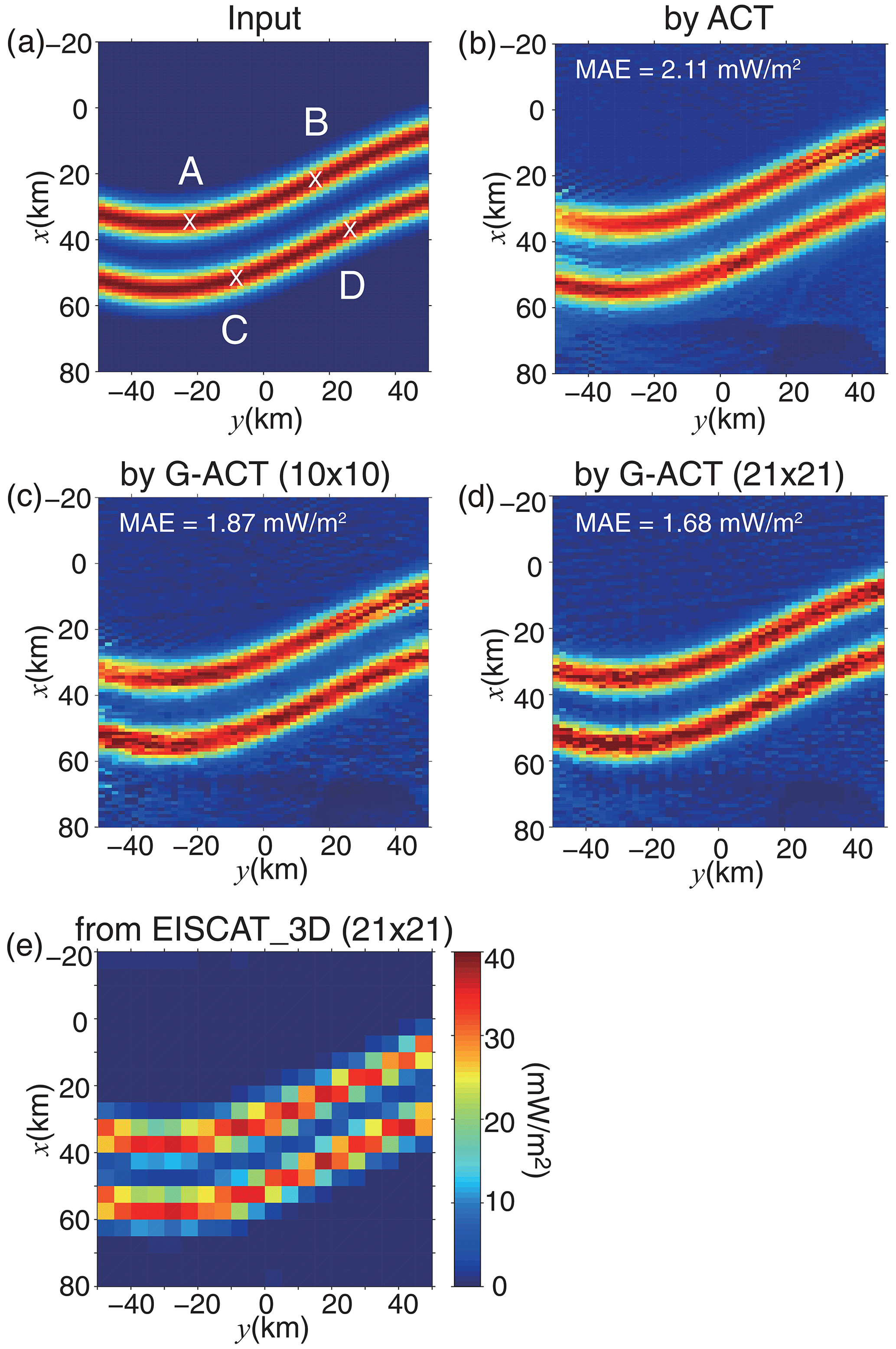
Figure 5(a) Horizontal distribution of the incident auroral electrons' total energy flux (Q0). Points A ([x,y] = [35, −22 km]), B ([x,y] = [23, 16 km]), C ([x,y] = [52, −8 km]), and D ([x,y] = [38, 16 km]) indicate the locations where the reconstructed height profiles of the electron density and energy spectra of the incident electrons are shown in this paper. (b) Q0 reconstructed from five ALIS images using the ACT method. (c) Q0 reconstructed by the G-ACT method using five ALIS images and the electron density from 10 × 10 beams of the EISCAT_3D radar. (d) Q0 reconstructed by the G-ACT method using five ALIS images and the electron density from 21 × 21 beams of the EISCAT_3D radar. (e) Q0 reconstructed only from the electron density from 21 × 21 beams of the EISCAT_3D radar.
The MAE was used for evaluating the reconstruction of the total energy flux, because the total energy flux includes values close to zero and thus the MAPE was unsuitable for it. The MAE was calculated by using all data in the evaluation area (−20 km < x < 80 km, −50 km < y < 50 km). The MAE values are shown in each panel of Fig. 5. The MAE for the ACT reconstruction was 2.11 mW m−2.
Figure 5c shows Q0 as reconstructed by G-ACT using both the ALIS images and the electron density data from the 10 × 10 beams of the EISCAT_3D radar. In this panel, the underestimation of Q0 at the center of each arc and the overestimation of Q0 between the two arcs brought by the normal ACT were significantly improved (MAE = 1.87 mW m−2). To more clearly show the impact of the electron density data on the improvement, we tested the case that the radar scanned the same area with 21 × 21 beams. Figure 5d presents Q0 reconstructed by G-ACT using the electron density from the 21 × 21 beams. It is evident that Q0 reconstructed by G-ACT is more accurate than that reconstructed by ACT (MAE = 1.68 mW m−2). The Q0 value at (x, y) = (45, −20 km) between the two arcs was improved to 4.36 mW m−2 (2.29 mW m−2) by the G-ACT method with the electron density data from the 10 × 10 beams (21 × 21 beams) of the EISCAT_3D radar.
Figure 5e shows Q0 derived from only the electron density data from the 21 × 21 beams of the EISCAT_3D radar. A larger spatial grid size ( km, Δz=3 km) was used for this inverse analysis. Since the spatial distribution of the electron density data from the radar was much sparser than the grid size for the ACT and G-ACT cases (i.e., Δx=1 km, km), a larger grid size was required to collect enough electron density data to solve the inverse problem, even for the 21 × 21 beam scan. The two discrete arcs were roughly reconstructed; however, the horizontal resolution was too low to resolve the fine-scale structure of the arcs.
Figure 6 shows height profiles of the electron density along the field lines at the locations (A, B, C, and D) shown in Fig. 5a. These locations were selected to emphasize the difference in the reconstruction between the normal ACT and G-ACT methods. The black line represents the true profile of the electron density, which was derived by the forward analysis using the incident electrons described in Sect. 2.2. The red squares show the modelled electron density data from the 10 × 10 beams of the EISCAT_3D radar. Several radar data exist along the field line at these locations. It is difficult to estimate the energy distribution of the precipitating electrons as well as the height distribution of the electron density from such few data; this is why the large grid size was used for the inversion from the EISCAT_3D radar data (Fig. 5e). The green crosses and blue circles correspond to the electron density reconstructed by the normal ACT and G-ACT methods, respectively. The spatial distribution of the electron density data obtained from only the optical images by ACT is much denser than those from the EISCAT_3D radar. However, the electron density is smaller than the true values, especially above the height of the peak density, which is consistent with the underestimation of Q0 (Fig. 5b). The underestimation of the electron density was significantly modified by G-ACT using the EISCAT_3D data. What is most important here is that the electron density can be interpolated at a much higher spatial resolution than that expected from only the EISCAT_3D radar.
The MAPE was used for evaluating the reconstructed electron density because it has a wide scale from 1010 to 1012 m−3, and the MAE was unsuitable for it. The MAPE values are shown in each panel of Fig. 6. The MAPE values for the electron density reconstructed by G-ACT are smaller than those by ACT at all the locations.
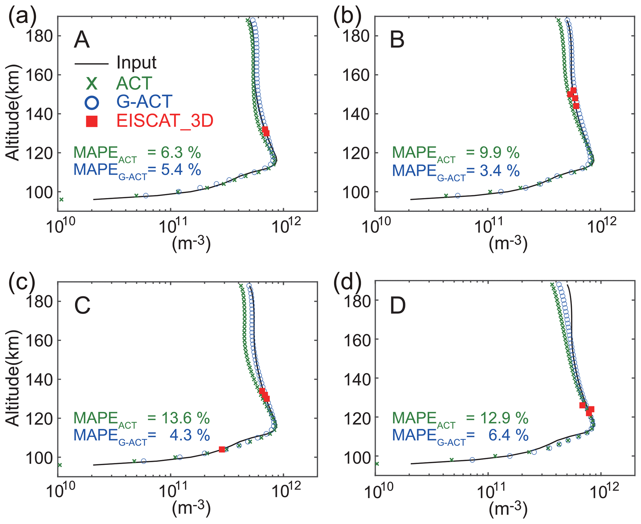
Figure 6Height profile of the ionospheric electron density at the points (a) A, (b) B, (c) C, and (d) D, which are shown in Fig. 5a. The black curve and solid red squares represent the electron density derived from the incident auroral electrons and modelled observational data from the EISCAT_3D radar (10 × 10 beams), respectively. Green crosses and blue circles show the electron density reconstructed by the ACT and G-ACT methods, respectively.
Figure 7 shows the energy distribution of the differential number flux of precipitating electrons at A, B, C, and D, as reconstructed by the ACT and G-ACT methods. The modelled electron density data from the 10 × 10 beams was used for the G-ACT analysis. This figure indicates that the differential flux reconstructed by the normal ACT tends to be underestimated in the energy range lower than the peak energy (E0). The underestimation of the differential flux was modified by G-ACT, particularly at the energy corresponding to the altitude where the electron density was obtained from the radar. In the assumed situation, the reconstruction results from G-ACT tends to be better also at the other points (except for A, B, C, and D) than those from ACT. Again, the MAPE was used for evaluating the reconstructed differential flux. Although the MAPE values for the differential flux are greater compared with those for the electron density profiles, the MAPE values for the G-ACT reconstruction are smaller than those for the ACT reconstruction at all the locations.
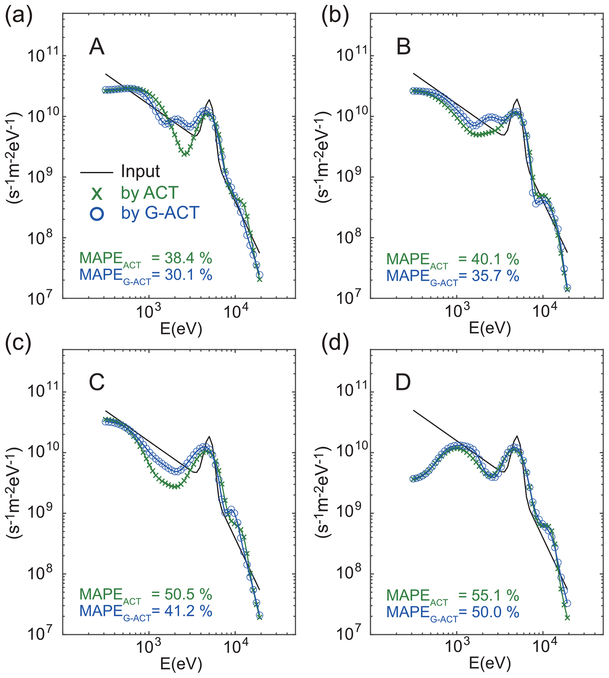
Figure 7Energy distribution of the differential number flux of the incident electrons at points (a) A, (b) B, (c) C, and (d) D, which are shown in Fig. 5a. The black curve shows the energy distribution of the incident electrons. Green crosses and blue circles show the differential number flux reconstructed using the ACT and G-ACT methods, respectively.
Figure 8a and b show Q0 as reconstructed by the ACT and G-ACT methods using data from three ALIS stations (Kiruna, Silkkimuotka, and Tjautjas). All three stations are located to the south of the discrete arcs. Under this condition, it was difficult for ACT to reconstruct the neighboring multiple arcs precisely from the images, because they overlap and cannot be distinguished from each other (MAE = 4.46 mW m−2). However, it was demonstrated that the G-ACT method using the electron density from the radar is capable of reconstructing the Q0 of multiple arcs. The underestimation of Q0 for both of the two arcs was greatly improved (MAE = 3.19 mW m−2), although it still remained because the radar beams were somewhat sparse. Again, we tested the 21 × 21 beam scan case on a trial basis. The reconstructed Q0 was better improved for both arcs (Fig. 8c; MAE = 1.86 mW m−2). Figure 8d and e show the reconstructions made by ACT and G-ACT when using data from two ALIS stations (Kiruna and Silkkimuotka). In this case, ACT was not able to separate the two discrete arcs, and the northern arc disappeared (MAE = 5.87 mW m−2). The northern arc was partially reconstructed by the G-ACT method; however, the reconstruction was still difficult in the 10 × 10 beam scan case (MAE = 3.97 mW m−2). Even in such a case, if a sufficient number of electron density data were available, the G-ACT method was able to reconstruct the Q0 of the two arcs very well (Fig. 8f; MAE = 1.80 mW m−2).
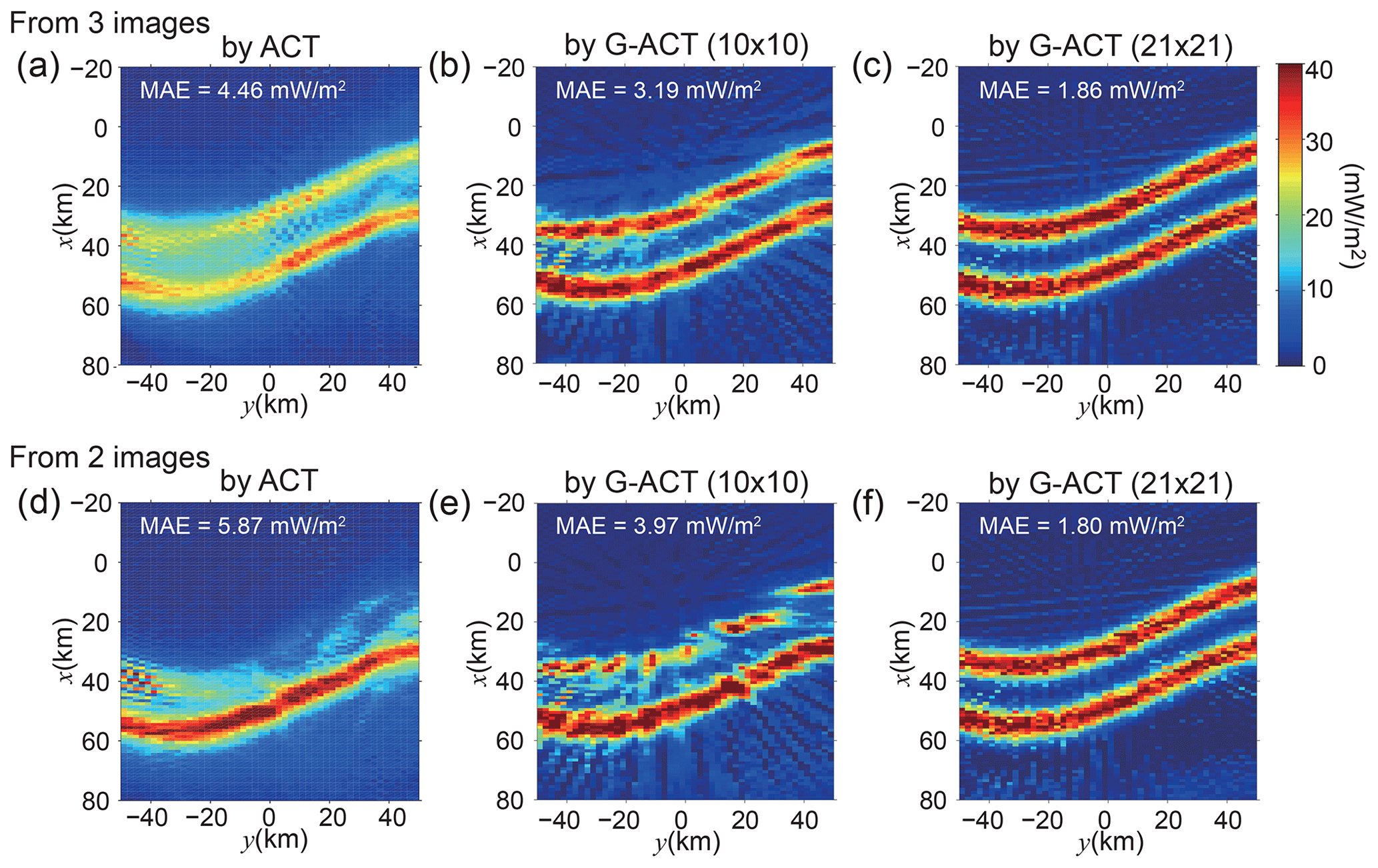
Figure 8Upper panels show the total energy flux (Q0) of the incident electrons reconstructed by using three ALIS images (Kiruna, Silkkimuotka, and Tjautjas). (a) Q0 reconstructed by the normal ACT, (b) by G-ACT using the electron density data from 10 × 10 beams, and (c) by G-ACT using the electron density data from 21 × 21 beams. Lower panels show Q0 reconstructed by using two ALIS images (Kiruna and Silkkimuotka). Panels (d), (e), and (f) were obtained by the same method as panels (a), (b), and (c), respectively.
Figure 9 shows the height profiles of the electron density at A and B. The upper and lower panels show the reconstruction results obtained by using three and two ALIS stations, respectively. It can be confirmed that the electron density data obtained from the EISCAT_3D radar were effectively used to improve the reconstructed result by the normal ACT, particularly around the altitude where the radar data exist. Although the electron density reconstructed by ACT with a few images is much lower than the true value, G-ACT enables the underestimation to be corrected. It was confirmed that the MAPE values for the reconstruction results by G-ACT were much smaller than those by ACT at all the cases.
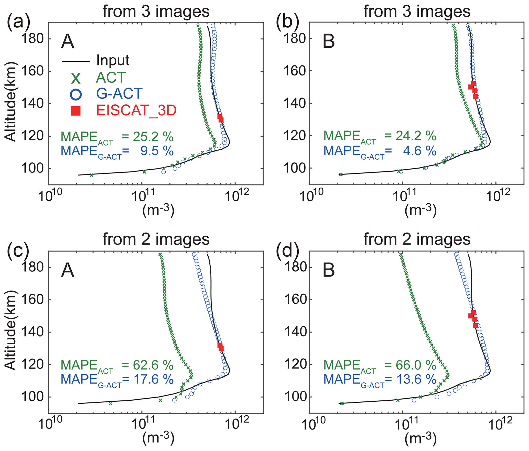
Figure 9Height profile of the ionospheric electron density. The format of this figure is similar to that of Fig. 6. Panels (a) and (b) indicate the electron density reconstructed by using three ALIS images (Kiruna, Silkkimuotka, and Tjautjas) at A and B, respectively. Panels (c) and (d) show the electron density reconstructed by using two ALIS images (Kiruna and Silkkimuotka) at A and B.
The EISCAT_3D radar can observe the ionospheric parameters at a much higher spatiotemporal resolution than the existing EISCAT radar. However, if one is interested in the auroral phenomena that have a horizontal scale larger than several tens of kilometers (such as growth-phase arcs, multiple arcs, spirals, westward-traveling surges, and omega bands), the spatial distribution of the ionospheric electron density data obtained by the beam scan of the EISCAT_3D radar may be too sparse to study the fine-scale structures inside the auroras. It is evident that the horizontal spatial resolution is too low to capture both the entire structure and fine-scale structure of the aurora (e.g., Fig. 5e).
The G-ACT method that combines the electron density data with the optical images may enable us to interpolate the electron density data at a much higher spatial resolution than that observed by the EISCAT_3D radar. In particular, this method is effective for the reconstruction of the 3D fine-scale structure of an aurora over a wide horizontal area at high temporal resolution. For instance, this method can provide the fine horizontal structure of the height-integrated ionospheric conductivity of mesoscale (10–1000 km) auroral phenomena at short sampling intervals. This indicates that it is possible to estimate the 3D current system of such auroral phenomena by using the magnetic field measured by a ground-based magnetometer network or the ionospheric electric field from radars (e.g., Vanhamäki and Amm, 2007).
Since the auroral images usually include observational noise, it is often difficult to reconstruct the auroral 3D distribution precisely by using the ACT method. As for the multiple arcs assumed in this study, the total energy flux of the precipitating electrons reconstructed by ACT was underestimated inside the discrete arcs. This is because the two neighboring arcs overlapped when viewed from several imagers and were difficult to perfectly separate. In Figure 5b, the reconstructed electron flux between the arcs was greater than the modelled flux; instead, the flux inside the arcs decreased. When the multiple arcs overlapped from all imagers, it was quite difficult for ACT to distinguish them from each other (Fig. 8). Of course, the reconstruction result depends on the condition such as the relative position of the aurora and the imagers, the noise level, and the shape of the aurora, and different conditions cause the reconstructed electron flux to be overestimated. We demonstrated that G-ACT can significantly reduce the reconstruction errors caused by ACT.
Here, we discuss the timescale of auroral phenomena to which the G-ACT method is applicable. We estimated the integration time required for observing the ionospheric electron density with the EISCAT_3D radar by Eqs. (63), (65), and (66) of Virtanen (2011). It was assumed that the range resolution is 2 km, the full width at half maximum (FWHM) of the beam is 1.4°, the observation frequency is 233 MHz, and the transmitter power is 3.5 MW, which corresponds to the power in the first stage of the EISCAT_3D radar. Then, the integration time needed to achieve the standard deviation of 5 % is less than 0.05 s per beam in the altitude range of 90–200 km when the electron density is greater than 1.0 × 10¹¹ m−3. Thus, the 10 × 10 beam scan assumed in this study takes about 5 s.
The interpulse period (IPP) between the pulses of the EISCAT_3D radar is about 5 ms for the E-region ionosphere observation. Thus, if a 16-bit pulse code is used, the minimum temporal resolution becomes 0.08 s per beam, resulting in 8 s for the 10 × 10 beam scan. In practice, the temporal resolution depends on the pulse code and background electron density; therefore, the 10 × 10 beam scan of the electron density in the E-region ionosphere may be made in less than 5 s.
The temporal resolution of the optical imager depends on the performance of the imager, the wavelength of the filter, the auroral emission intensity, etc. Since the monochromatic images are required for the G-ACT analysis, the temporal resolution of high-sensitivity imagers (e.g., electron-multiplying CCD (EMCCD) imagers) with the monochromatic filters is usually a few seconds or less and can be higher than that of the 10 × 10 beam scan of the radar. For example, Fukizawa et al. (2022) reconstructed the 3D distribution of pulsating aurora every 2 s by ACT using the 427.8 nm auroral images. Furthermore, 10 Hz sampling monochromatic all-sky imagers observing 427.8 nm auroral emission have been operative in Tromsø, Norway (Hosokawa et al., 2023).
In addition, the steady state of the electron density was assumed in this study, as given by
in the E-region ionosphere. Here, q is the ion production rate, Ne is the electron density, and α is the effective recombination coefficient. The steady-state condition is satisfied when the incident electron precipitation does not change over timescales longer than the ion recombination time constant, (e.g., Semeter and Kamalabadi, 2005). It is well known that α has a large uncertainty (Penman et al., 1979). By using α used by Semeter and Kamalabadi (2005), τ is between 16 and 50 s in the altitude of 90–190 km when the electron density is 1.0 × 10¹¹ m−3, and τ decreases as the electron density increases. Thus, the reconstruction results by G-ACT using the current model are valid if the auroral arcs are stable for a longer time than τ. However, it is straightforward to add the time derivative term of the electron density to our model (i.e., , because this term can be estimated by the continuous observation of the electron density. Such a modified model is available if is stable during the data acquisition interval. We will examine the modification of the model in the near future.
The mesoscale auroras that we mentioned here have the following typical drift speeds; 70–170 m s−1 for the equatorward drift of the growth-phase arcs (Karlsson et al., 2020), 1–2 km s−1 for the westward-traveling surges (Kamide and Baumjohann, 1993), and 200–800 m s−1 for the eastward drift of the omega bands (Vokhmyanin et al., 2021) at the ionospheric altitude. Pulsating auroras are also mesoscale diffuse aurora, which switch on and off with a quasiperiodic oscillation period of 2–20 s (Lessard, 2012). To study auroral phenomena with relatively fast temporal variations, the number and direction of the beams need to be adjusted. In such situations, simulation studies as shown in this study may be useful in planning observations.
We demonstrated via numerical simulation that the combination of optical imagers and the EISCAT_3D radar is very powerful for the study of aurora physics, since they have a complementary relationship with each other. G-ACT, which was used to reconstruct the 3D distribution of auroras (corresponding to the horizontal 2D distribution of the electron energy spectra) from multi-instrument data, can be applied as a technique to take advantage of the optical image data effectively. It has the capability to interpolate the electron density observed by the EISCAT_3D radar at a higher spatial resolution, in particular for mesoscale (10–1000 km) auroral phenomena. G-ACT enables auroral phenomena to be better reconstructed than when the normal ACT is used. Even if ACT cannot reconstruct the auroral distribution precisely, G-ACT may allow us to reduce the reconstruction error. Therefore, it is important to construct multi-point monochromatic imager networks that cover the observation region of the EISCAT_3D radar in the near future.
The data used in this study are available at https://doi.org/10.5281/zenodo.10872240 (Tanaka and Ogawa, 2024).
YT conducted numerical simulation and prepared the manuscript with contributions from all co-authors. YO provided the modelled ionospheric electron density data from the EISCAT_3D radar and contributed to the discussion. AK, TA, BG, UB, TS, GU, and SS contributed to the discussion and interpretation of the simulation results.
The contact author has declared that none of the authors has any competing interests.
Publisher’s note: Copernicus Publications remains neutral with regard to jurisdictional claims made in the text, published maps, institutional affiliations, or any other geographical representation in this paper. While Copernicus Publications makes every effort to include appropriate place names, the final responsibility lies with the authors.
This study was supported by JSPS KAKENHI grant numbers JP17K05672, JP21H01152, and JP22H00173. This work was supported in part by the Inter-university Upper atmosphere Global Observation NETwork (IUGEONET) project (http://www.iugonet.org/, last access: 5 May 2024). EISCAT is an international association supported by research organizations in China (CRIRP), Finland (SA), Japan (NIPR), Norway (NFR), Sweden (VR), and the United Kingdom (UKRI). ALIS is supported by the Swedish Research Council. The production of this paper was supported by an NIPR publication subsidy.
This research has been supported by JSPS KAKENHI (grant nos. JP17K05672, JP21H01152, and JP22H00173).
This paper was edited by Keisuke Hosokawa and reviewed by M. J. Kosch and one anonymous referee.
Alken, P., Thébault, E., Beggan, C. D., Amit, H., Aubert, J., Baerenzung, J., Bondar, T. N., Brown, W. J., Califf, S., Chambodut, A., Chulliat, A., Cox, G. A., Finlay, C. C., Fournier, A., Gillet, N., Grayver, A., Hammer, M. D., Holschneider, M., Huder, L., Hulot, G., Jager, T., Kloss, C., Korte, M., Kuang, W., Kuvshinov, A., Langlais, B., Léger, J.-M., Lesur, V., Livermore, P. W., Lowes, F. J., Macmillan, S., Magnes, W., Mandea, M., Marsal, S., Matzka, J., Metman, M. C., Minami, T., Morschhauser, A., Mound, J. E., Nair, M., Nakano, S., Olsen, N., Pavón-Carrasco, F. J., Petrov, V. G., Ropp, G., Rother, M., Sabaka, T. J., Sanchez, S., Saturnino, D., Schnepf, N. R., Shen, X., Stolle, C., Tangborn, A., Tøffner-Clausen, L., Toh, H., Torta, J. M., Varner, J., Vervelidou, F., Vigneron, P., Wardinski, I., Wicht, J., Woods, A., Yang, Y., Zeren, Z., and Zhou, B.: International Geomagnetic Reference Field: the thirteenth generation, Earth Planet. Space, 73, 49, https://doi.org/10.1186/s40623-020-01288-x, 2021.
Aso, T., Ejiri, M., Urashima, A., Miayoka, H., Steen, Å., Brändström, U., and Gustavsson, B.: First results of auroral tomography from ALIS-Japan multi-station observations in March, 1995, Earth Planet. Space, 50, 81–86, https://doi.org/10.1186/BF03352088, 1998.
Aso, T., Gustavsson, B., Tanabe, K., Brändström, U., Sergienko, T. and Sandahl, I.: A proposed Bayesian model on the generalized tomographic inversion of aurora using multi-instrument data, Proc. 33rd Annual European Meeting on Atmospheric Studies by Optical Methods, Swedish Institute of Space Physics, IRF Sci. Rep., 292, 105–109, ISBN 978-91-977255-1-4, 2008.
Brändström, U.: The Auroral Large Imaging System – Design, operation and scientific results, Kiruna, Swedish Institute of Space Physics, IRF Sci. Rep., 279, ISBN 91-7305-405-4, 2003.
Ellis, P. and Southwood, D. J.: Reflection of Alfvén waves by non-uniform ionospheres, Planet. Space Sci., 31, 107–117, https://doi.org/10.1016/0032-0633(83)90035-1, 1983.
Fukizawa, M., Sakanoi, T., Tanaka, Y., Ogawa, Y., Hosokawa, K., Gustavsson, B., Kauristie, K., Kozlovsky, A., Raita, T., Brändström, U., and Sergienko, T.: Reconstruction of precipitating electrons and three-dimensional structure of a pulsating auroral patch from monochromatic auroral images obtained from multiple observation points, Ann. Geophys., 40, 475–484, https://doi.org/10.5194/angeo-40-475-2022, 2022.
Glaßmeier, K.-H.: On the influence of ionospheres with non-uniform conductivity distribution on hydromagnetic waves, J. Geophys., 54, 125–137, https://journal.geophysicsjournal.com/JofG/article/view/157, 1984.
Gustavsson, B.: Tomographic inversion for ALIS noise and resolution, J. Geophys. Res., 103, 26621–26632, https://doi.org/10.1029/98JA00678, 1998.
Gustavsson, B., Steen, Å., Sergienko, T., and Brändström, B.: Estimate of auroral electron spectra, the power of ground-based multi-station optical measurements, Phys. Chem. Earth Pt. C, 26, 189–194, https://doi.org/10.1016/S1464-1917(00)00106-9, 2001.
Hedin, A. E.: Extension of the MSIS thermosphere model into the middle and lower atmosphere, J. Geophys. Res., 96, 1159–1172, https://doi.org/10.1029/90JA02125, 1991.
Hosokawa, K., Oyama, S.-I., Ogawa, Y., Miyoshi, Y., Kurita, S., Teramoto, M., Nozawa, N., Kawabata, T., Kawamura, Y., Tanaka, Y.-M., Miyaoka, H., Kataoka, R., Shiokawa, K., Brändström, U., Turunen, E., Raita, T., Johnsen, M. G., Hall, C., Hampton, D., Ebihara, Y., Kasahara, Y., Matsuda, S., Shinohara, I., and Fujii, R.: A ground-based instrument suite for integrated high-time resolution measurements of pulsating aurora with Arase, J. Geophys. Res.-Space, 128, e2023JA031527, https://doi.org/10.1029/2023JA031527, 2023.
Itonaga, M. and Kitamura, T.: Effect of non-uniform ionospheric conductivity distributions on Pc 3–5 magnetic pulsations – Alfvén wave incidence, J. Geomag. Geoelectr., 40, 1413–1435, https://doi.org/10.5636/jgg.40.1413, 1988.
Janhunen, P.: Reconstruction of electron precipitation characteristics from a set of multiwavelength digital all-sky auroral images, J. Geophys. Res., 106, 18505–18516, https://doi.org/10.1029/2000JA000263, 2001.
Kamide, Y. and Baumjohann, W.: Magnetosphere-Ionosphere Coupling, Springer-Verlag, New York, https://doi.org/10.1007/978-3-642-50062-6, 1993.
Kamide, Y., Richmond, A. D., and Matsushita, S.: Estimation of ionospheric electric fields, ionospheric currents, and field-aligned currents from ground magnetic records, J. Geophys. Res., 86, 801–813, https://doi.org/10.1029/JA086iA02p00801, 1981.
Karlsson, T., Andersson, L., Gillies, D.M., Lynch, K., Marghitu, O., Partamies, N., Sivadas, N., and Wu, J.: Quiet, Discrete Auroral Arcs – Observations, Space Sci. Rev., 216, 16, https://doi.org/10.1007/s11214-020-0641-7, 2020.
Lessard, M. R.: A Review of Pulsating Aurora, in: Auroral Phenomenology and Magnetospheric Processes: Earth And Other Planets, edited by: Keiling, A., Donovan, E., Bagenal, F., and Karlsson, T., 55–68, AGU, Washington, D.C., American Geophysical Union, https://doi.org/10.1029/2011GM001187, 2012.
McCrea, I., Aikio, A., Alfonsi, L., Belova, E., Buchert, S., Clilverd, M., Engler, N., Gustavsson, B., Heinselman, C., Kero, J., Kosch, M., Lamy, H., Leyser, T., Ogawa, Y., Oksavik, K., Pellinen-Wannberg, A., Pitout, F., Rapp, M., Stanislawska, I., and Vierinen, J.: The science case for the EISCAT_3D radar, Prog. Earth Planet. Sci., 2, 21, https://doi.org/10.1186/s40645-015-0051-8, 2015.
Ogawa, Y., Tanaka, Y., Kadokura, A., Hosokawa, K., Ebihara, Y., Motoba, T., Gustavsson, B., Brändström, U., Sato, Y., Oyama, S., Ozaki, M., Raita, T., Sigernes, F., Nozawa, S., Shiokawa, K., Kosch, M., Kauristie, K., Hall, C., Suzuki, S., Miyoshi, Y., Gerrard, A., Miyaoka, H., and Fujii, R.: Development of low-cost multi-wavelength imager system for studies of aurora and airglow, Polar Sci., 23, 100501, https://doi.org/10.1016/j.polar.2019.100501, 2020.
Penman, J. M., Hargreaves, J. K., and McIlwain, C. E.: The relation between 10 to 80 keV electron precipitation observed at geosynchronous orbit and auroral radio absorption observed with riometers, Planet. Space Sci., 27, 445–451, https://doi.org/10.1016/0032-0633(79)90121-1, 1979.
Rees, M. H.: Physics and chemistry of the upper atmosphere, Cambridge University Press, edited by: Houghton, J. T., Rycroft, M. J., and Dessler, A. J., New York, https://doi.org/10.1017/CBO9780511573118, 1989.
Simon Wedlund, C., Lamy, H., Gustavsson, B., Sergienko, T., and Brändström, U.: Estimating energy spectra of electron precipitation above auroral arcs from ground-based observations with radar and optics, J. Geophys. Res., 118, 3672–3691, https://doi.org/10.1002/jgra.50347, 2013.
Semeter, J. and Kamalabadi, F.: Determination of primary electron spectra from incoherent scatter radar measurements of the auroral E region, Radio Sci., 40, RS2006, https://doi.org/10.1029/2004RS003042, 2005.
Sergienko, T. and Ivanov, V.: A new approach to calculate the excitation of atmospheric gases by auroral electron impact, Ann. Geophys., 11, 717–727, 1993.
Stone, M.: Cross-validatory choice and assessment of statistical predictions (with discussion), J. R. Stat. Soc. Ser. B, 38, 102–102, https://doi.org/10.1111/j.2517-6161.1976.tb01573.x, 1974.
Strickland, D. J., Daniell Jr., R. E., Jasperse, J. R., and Basu, B.: Transport-theoretic model for the electron-proton-hydrogen atom aurora, 2. Model results, J. Geophys. Res., 98, 21533–21548, https://doi.org/10.1029/93JA01645, 1993.
Syrjäsuo, M.: FMI All-Sky Camera Network, Geophysical Publications Nr. 52, Finnish Meteorological Institute, ISBN 951-697-543-7, 2001.
Tanaka, Y. and Ogawa, Y.: Dataset for “Application of Generalized – Aurora Computed Tomography to the EISCAT_3D project”, Annales Geophysicae (1.0), Zenodo [data set], https://doi.org/10.5281/zenodo.10872240, 2024.
Tanaka, Y.-M., Aso, T., Gustavsson, B., Tanabe, K., Ogawa, Y., Kadokura, A., Miyaoka, H., Sergienko, T., Brändström, U., and Sandahl, I.: Feasibility study on Generalized-Aurora Computed Tomography, Ann. Geophys., 29, 551–562, https://doi.org/10.5194/angeo-29-551-2011, 2011.
Vanhamäki, H. and Amm, O.: A new method to estimate ionospheric electric fields and currents using data from a local ground magnetometer network, Ann. Geophys., 25, 1141–1156, https://doi.org/10.5194/angeo-25-1141-2007, 2007.
Virtanen, I. I.: Plasma parameter error estimates for multi-static IS radars, 132–144, EISCAT_3D design HB preliminary version 0.1, 2011.
Vokhmyanin, M., Apatenkov, S., Gordeev, E., Andreeva, V., Partamies, N., Kauristie, K., and Juusola, L.: Statistics on omega band properties and related geomagnetic variations, J. Geophys. Res.-Space, 126, e2021JA029468, https://doi.org/10.1029/2021JA029468, 2021.
Wannberg, U. G., Eliasson, L., Johansson, J., Wolf, I., Andersson, H., Bergqvist, P., Häggström, I., Iinatti, T., Laakso, T., Larsen, R., Markkanen, J., Marttala, I., Postila, M., Turunen, E., van Eyken, A., Vanhainen, L.-G., Westman, A., Behlke, R., Belyey, V., Grydeland, T., Gustavsson, B., La Hoz, C., Borg, J., Delsing, J., Johansson, J., Larsmark, M., Lindgren, T., Lundberg, M., Finch, I., Harrison, R. A., McKay, D., Puccio, W., Renkwitz, T., Grydeland, T., Gustavsson, B., Postila, M., and van Eyken, A.: Eiscat_3D: A next-generation European radar system for upper-atmosphere and geospace research, URSI Radio Sci. Bull., 333, 75–88, 2010.