Statistical study of linear magnetic hole structures near Earth

The Magnetospheric Multiscale mission (MMS1) data for 8 months in the winter periods of 2017–2018 and 2018–2019, when MMS had its apogee in the upstream solar wind of the Earth's bow shock, are used to study linear magnetic holes (LMHs). These LMHs are characterized by a magnetic depression of more than 50 % and a rotation of the background magnetic field of less then 10^∘. A total of 406 LMHs are found and, based on their magnetoplasma characteristics, are split into three categories: cold (increase in density, little change in ion temperature), hot (increase in ion temperature, decrease in density) and sign change (at least one magnetic field component changes sign). The occurrence rate of LMHs is 2.3 per day. All LMHs are basically in pressure balance with the ambient plasma. Most of the linear magnetic holes are found in ambient plasmas that are stable against the mirror-mode generation, but only half of the holes are mirror-mode-stable inside.

1 Introduction

One of the structures in the interplanetary magnetic field (IMF) that can be found throughout the solar system is the magnetic hole (MH), first discussed by Turner et al. (1977). These are depressions in the magnetic field strength up to 90 % of the background magnetic field. Although Turner et al. (1977) did not have adequate plasma measurement, they assumed that these were diamagnetic structures. Theoretically this was discussed by Burlaga and Lemaire (1978), and later measurements have shown that increased plasma pressure in the MHs takes care of the pressure balance (see, for example, Burlaga et al., 1990; Winterhalter et al., 1995). A special case of MHs where the magnetic field direction does not change more than 10^∘ is called the linear magnetic hole (LMH; Turner et al., 1977).

The origin of (L)MHs is still not completely clear. These structures appear in the solar wind for high-plasma-β conditions, and they are most likely related to mirror modes (MMs) or might even be the end stage of MMs (Winterhalter et al., 1994). Winterhalter et al. (2000), for example, found that trains of MMs were observed in MM-unstable ambient plasma, but when the instability criterion was not fulfilled for the ambient plasma, there were only LMHs.

MMs occur in high-β plasmas with a temperature asymmetry $T_{⟂}>T_{\Vert }$ (Gary et al., 1993), and specifically the instability criterion for a bi-Maxwellian distribution is (Southwood and Kivelson, 1993)

$$\begin{array}{}\text{(1)}& R_{\mathrm{SK}}={\displaystyle \frac{T_{\mathrm{i}⟂}/T_{\mathrm{i}\Vert }}{\mathrm{1}+\mathrm{1}/{\mathit{\beta }}_{\mathrm{i}⟂}}}>\mathrm{1},\end{array}$$

where

$$\begin{array}{}\text{(2)}& {\mathit{\beta }}_{\mathrm{i}⟂}={\displaystyle \frac{n_{\mathrm{i}}{k}_{\mathrm{B}}{T}_{\mathrm{i}⟂}}{B^{\mathrm{2}}/\mathrm{2}{\mathit{\mu }}_{\mathrm{0}}}},\end{array}$$

with T_i⟂ and T_i‖ the perpendicular and parallel ion temperature, n_i the ion density, B the magnetic field strength, k_B Boltzmann's constant and μ₀ the permeability of vacuum. (For a more general discussion of the instability criterion, see, for example, Hellinger, 2007.) Stevens and Kasper (2007) found that LMHs mainly occurred in MM-stable regions (R_SK<1). This might lead to the conclusion that as soon as the plasma becomes MM-stable, the MMs start to diffuse/transform into MHs. Hasegawa and Tsurutani (2011) proposed a Bohm-like diffusion (Bohm et al., 1949) process taking place in the MMs, where the higher frequencies of the structure decay faster than the lower frequencies, and thereby the MMs grow in size as they move away from the generation location. The scale size of the MMs is then given by

$$\begin{array}{}\text{(3)}& \mathit{\lambda }\left(\mathcal{L}\right)={\mathit{\lambda }}_{\mathrm{0}}\left(\mathrm{1}+{\displaystyle \frac{{\mathit{\omega }}_{\mathrm{ic}}\mathcal{L}}{\mathrm{32}u}}\right),\end{array}$$

where λ₀ is the MM size at the source region, ℒ is the distance from the source region, ω_ic is the ion cyclotron frequency and u is the convection speed of the MMs. Schmid et al. (2014) showed that the growth of MMs in Venus's and comet 1P/Halley's magnetosheaths was well described by this process for pick-up ion species protons and water, respectively. It can be envisioned that through the growth of the MMs, the wave trains merge into larger structures, leading to MHs.

There have been many studies on the occurrence rate of LMHs throughout the solar system. In Table 1 the rates are listed from the inner solar system to the outer reaches. It is clear that most occurrence rates are about a few per day. However, it is difficult to compare the exact values listed. As an example, it is immediately obvious that occurrence rates differ strongly near Venus: Zhang et al. (2008) found a rate of 4.5 per day, whereas Volwerk et al. (2020) reported a rate of 1.0 per day. These studies were done for 2006 and 2007, respectively; the difference was not caused by changes in solar activity but by the selection criteria used: $\mathrm{\Delta }B/B>\mathrm{0.25}$ vs. 0.50 $\mathrm{\Delta }\mathit{\theta }<\mathrm{15}{}^{\circ }$ vs. 10^∘. This shows the necessity of studying these structures with one unified set of conditions; only then can precise physical statements be made about their characteristics and development (see also Klein and Burlaga, 1980).

Karlsson et al. (2020)Volwerk et al. (2020)Zhang et al. (2008)Sperveslage et al. (2000)Stevens and Kasper (2007)Turner et al. (1977)Xiao et al. (2014)Madanian et al. (2020)Sperveslage et al. (2000)Sperveslage et al. (2000)Winterhalter et al. (2000)Burlaga et al. (2007)

Table 1 Occurrence rates of magnetic holes in the solar wind throughout the system.

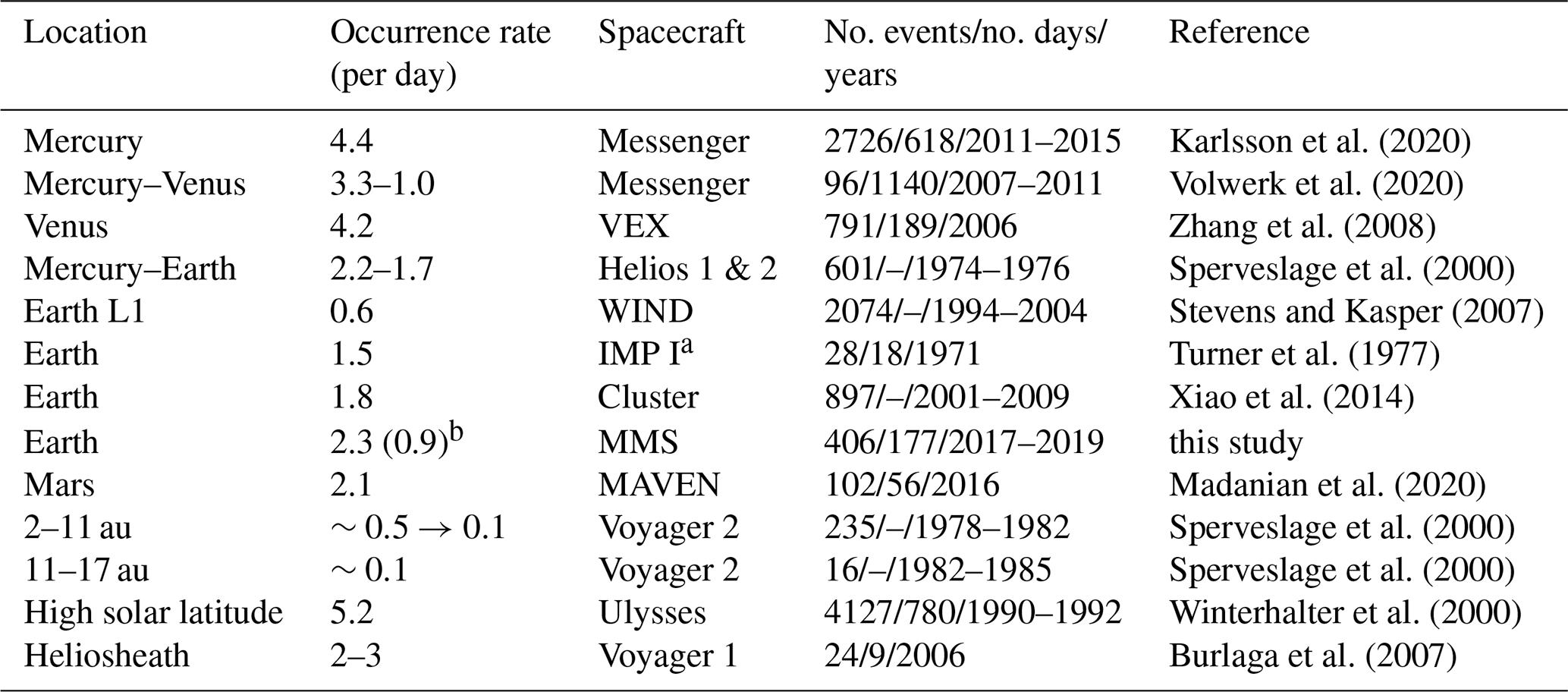
^a a.k.a. Explorer 43. ^b After exclusion of the sign change category, this number reduces to 0.9.

In this paper the Magnetospheric Multiscale (MMS; Burch et al., 2016) mission is used, for the winter seasons of 2017/18 and 2018/19, when the spacecraft had their apogee in the upstream solar wind. A statistical study is done for the occurrence rate and the characteristics of the LMH structures that are found in the data.

2 Instrumentation and data analysis

The MMS fluxgate magnetometer (FGM) fast data (Russell et al., 2016) are used with a sampling rate of 16 Hz, which are downsampled to 1 s resolution. The data are restricted to such time intervals that MMS had its apogee in the solar wind, i.e. November 2017 through March 2018 and December 2018 through March 2019. An additional limit was set to the location of the spacecraft, namely that it be farther out than 15 R_E, to avoid influence from the Earth's bow shock, which can move further outward in times of low solar wind pressure (Meziane et al., 2014). However this will not exclude the foreshock region from the data set, which extends much further upstream (Heppner et al., 1968; Greenstadt et al., 1968; Scarf et al., 1970).

The FGM data were then handled as in previous papers by Plaschke et al. (2018) and Volwerk et al. (2020) in order to find linear magnetic holes (LMHs).

1. The background magnetic field, B₃₀₀, is determined by a sliding window average over 300 s.

2. The data are smoothed by a sliding window average of 2 s, which gives B₂.

3. The ratio $\mathrm{\Delta }B/B_{\mathrm{300}}=(B_{\mathrm{300}}-B_{\mathrm{2}})/B_{\mathrm{300}}$ is calculated, and the lowest field depressions are selected that are at least 300 s apart.

4. The background field should be B₃₀₀≥2 nT.

5. The ratio $\mathrm{\Delta }B/B_{\mathrm{300}}>\mathrm{0.5}$.

6. The rotation of the magnetic field over the hole $\mathit{\theta }\le \mathrm{10}{}^{\circ }$.

All data are in geocentric solar equatorial (GSE) coordinates. This resulted in 406 LMH structures observed between 15 and 30 R_E from the Earth, an example of which can be seen in Fig. 1, and for all structures, plasma data are available.

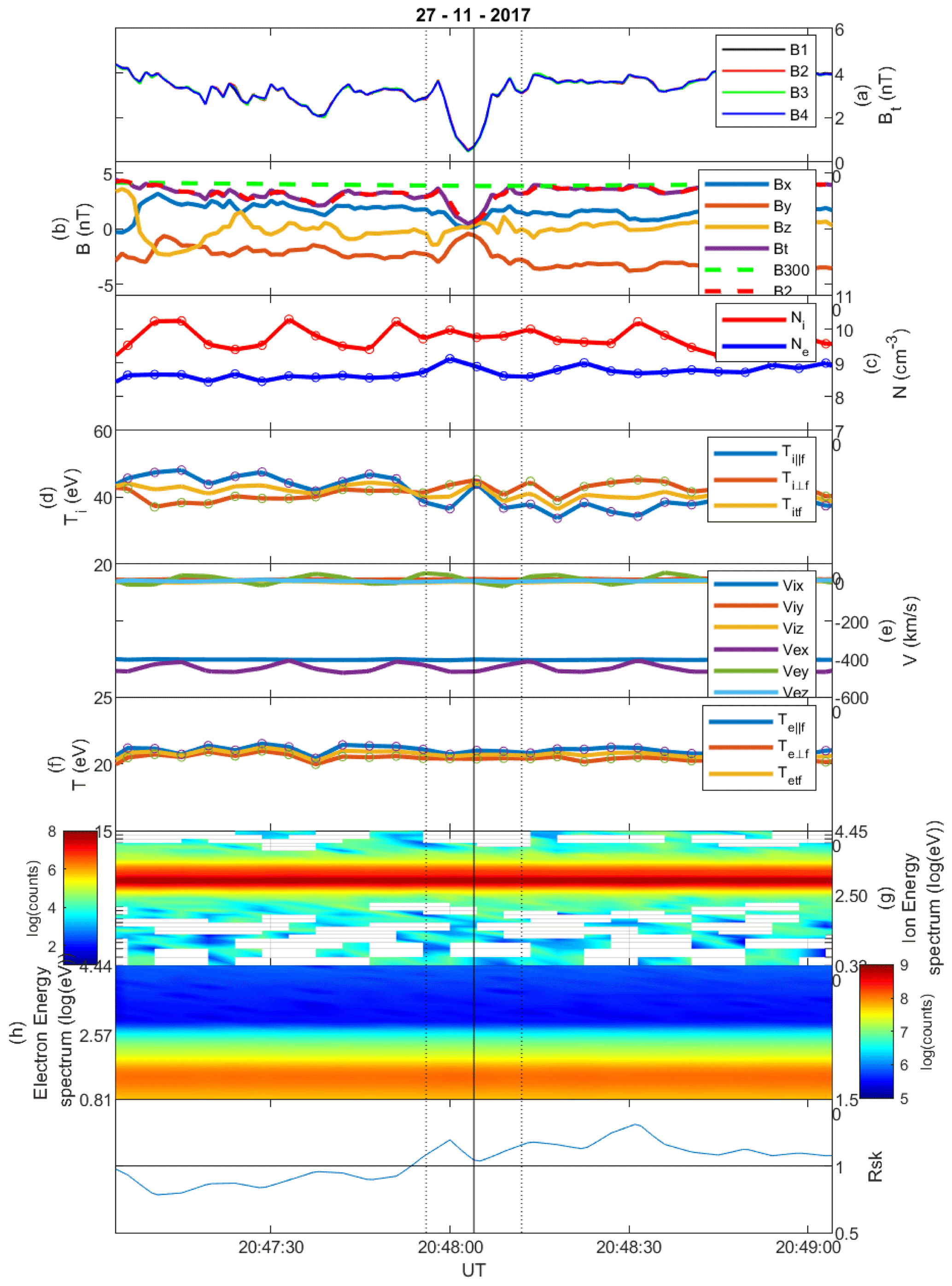
Figure 1 Linear magnetic hole on 27 November 2017, category cold. (a) The total magnetic field B_t for all four MMS spacecraft. (b) The magnetic field components with B₃₀₀ and B₂. (c) The fast-mode ion and electron density. (d) The parallel, perpendicular and total ion temperature in fast mode. (e) The fast-mode ion and electron velocity components. (f) The parallel, perpendicular and total electron temperature in fast mode. (g) The ion energy spectrogram. (h) The electron energy spectrogram. (i) The instability criterion R_SK.

As compared with previous papers (Plaschke et al., 2018; Volwerk et al., 2020), MMS has plasma data from the Fast Plasma Investigation (FPI; Pollock et al., 2016), with a temporal resolution for the fast mode of 4.5 s for ions and electrons. These measurements allow for the determination of the ion density and temperature inside the LMH structures. However, the FPI moments need to be looked at carefully because the FPI instrument was not developed for solar wind conditions. This means that the different parameters that are obtained from the instrument may be inaccurate. In order to check the quality of the FPI data, they can be compared with data from solar-wind-specialized missions such as Wind (Lin et al., 1995). Something similar occurs with the ARTEMIS mission (Angelopoulos, 2011), which has basically the same plasma instrument and only has a magnetospheric mode. Artemyev et al. (2018) compared 6 years of ARTEMIS data with the OMNI data set (King and Papitashvili, 2005). They found good correlation, within a factor of 2, between the ARTEMIS electron density and the OMNI ion density.

Bandyopadhyay et al. (2020) compared the FPI data with Wind mission data for one event. They found that there was a slight discrepancy for the proton density, whereas the proton velocity was in good agreement, and the proton temperature was underestimated. Recently, Roberts et al. (2021) presented a statistical study comparing the ion and electron data from FPI in the solar wind with the OMNI data. They found that the ion density was underestimated (up to a factor of 2 for densities greater than 10 cm⁻³) and the ion temperature was overestimated (up to a factor of 2). However, for the electrons, they found good agreement between the two data sets, assuming quasi-neutrality of the plasma to calculate the OMNI electron density from the OMNI ion density.

As FPI was not specifically developed for solar wind conditions, this also means that there can be spurious signals in the FPI data, such that the spin tone at ∼20 s is not removed correctly. This will then appear as ∼20 s variation in various plasma components such as density and velocity.

In this paper only the MMS1 data will be used, as the inter-spacecraft distance is too small to show any significant differences between the four spacecraft with respect to the structures that are investigated. Also, as there is only burst-mode data (at a resolution of 30 ms) for a small number of the identified structures, the fast-mode FPI data are used in this paper.

Taking together all the LMH structures, and determining the dwelling time of MMS in the region between 15 and 30, R_E gives an occurrence rate of 2.3 per day. This is close to what was found in previous studies: 1.5 per day (Turner et al., 1977), 1.7–2.2 per day (Sperveslage et al., 2000), 0.6 per day (Stevens and Kasper, 2007) and 1.8 per day (Xiao et al., 2014) (see also Table 1).

The occurrence rate is calculated as a function of the distance from Earth and is shown in Fig. 2 by blue lines (the other colours are defined further below). There is a strong variation in the occurrence rates, showing the randomness with which these structures appear.

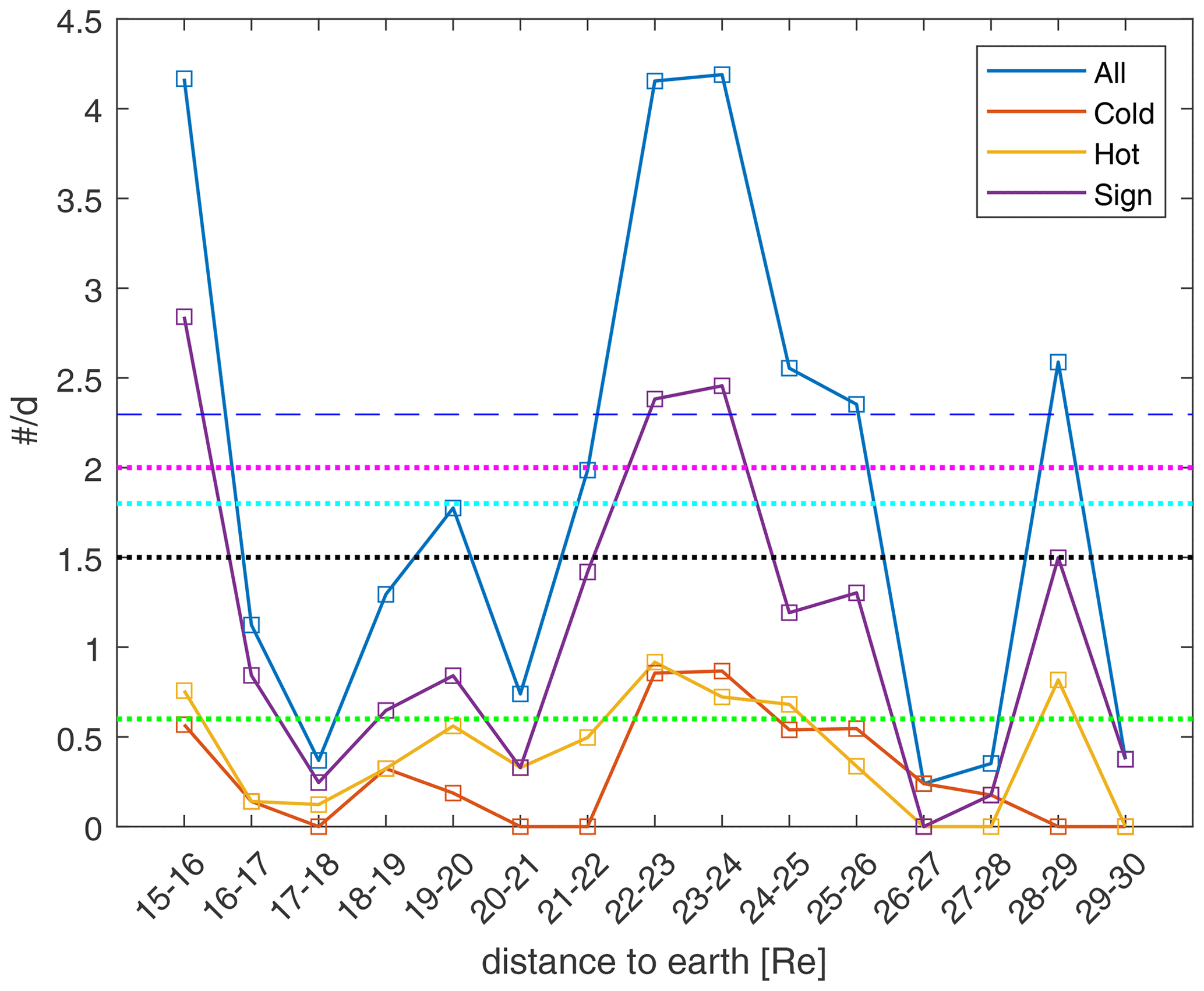
Figure 2 The occurrence rate of LMH structures as a function of the distance from Earth. The blue squares connected by blue lines show the occurrence rates for all structures. The red squares and line are for the cold LMHs, the yellow for the hot LMHs and the purple for sign change LMHs. The dashed blue line is the average occurrence rate (2.3 per day), and the dotted coloured lines are the daily occurrence rates from literature: 1.5 (black; Turner et al., 1977), 2.0 (magenta; Sperveslage et al., 2000), 0.6 (green; Stevens and Kasper, 2007) and 1.8 (cyan; Xiao et al., 2014).

The apparent temporal width, w, of the LMH structures in the time series is also determined during the search for the events, which corresponds to the full width at half maximum (FWHM). In Fig. 3 the distribution is shown, which peaks in the bins 5–10 and 10–15 s. This value agrees well with the highest occurrence of widths found between Mercury and Venus (Sperveslage et al., 2000; Volwerk et al., 2020).

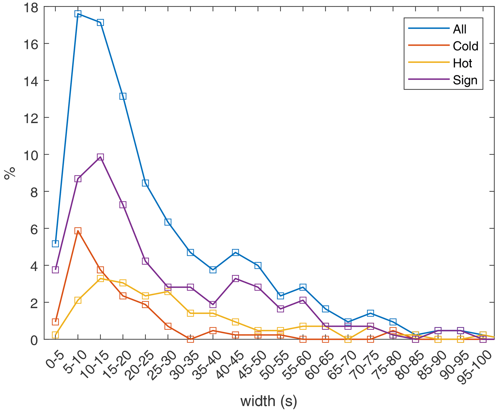
Figure 3 The distribution of the widths of the LMH structures in percentage of total events. The colour coding is the same as in Fig. 2.

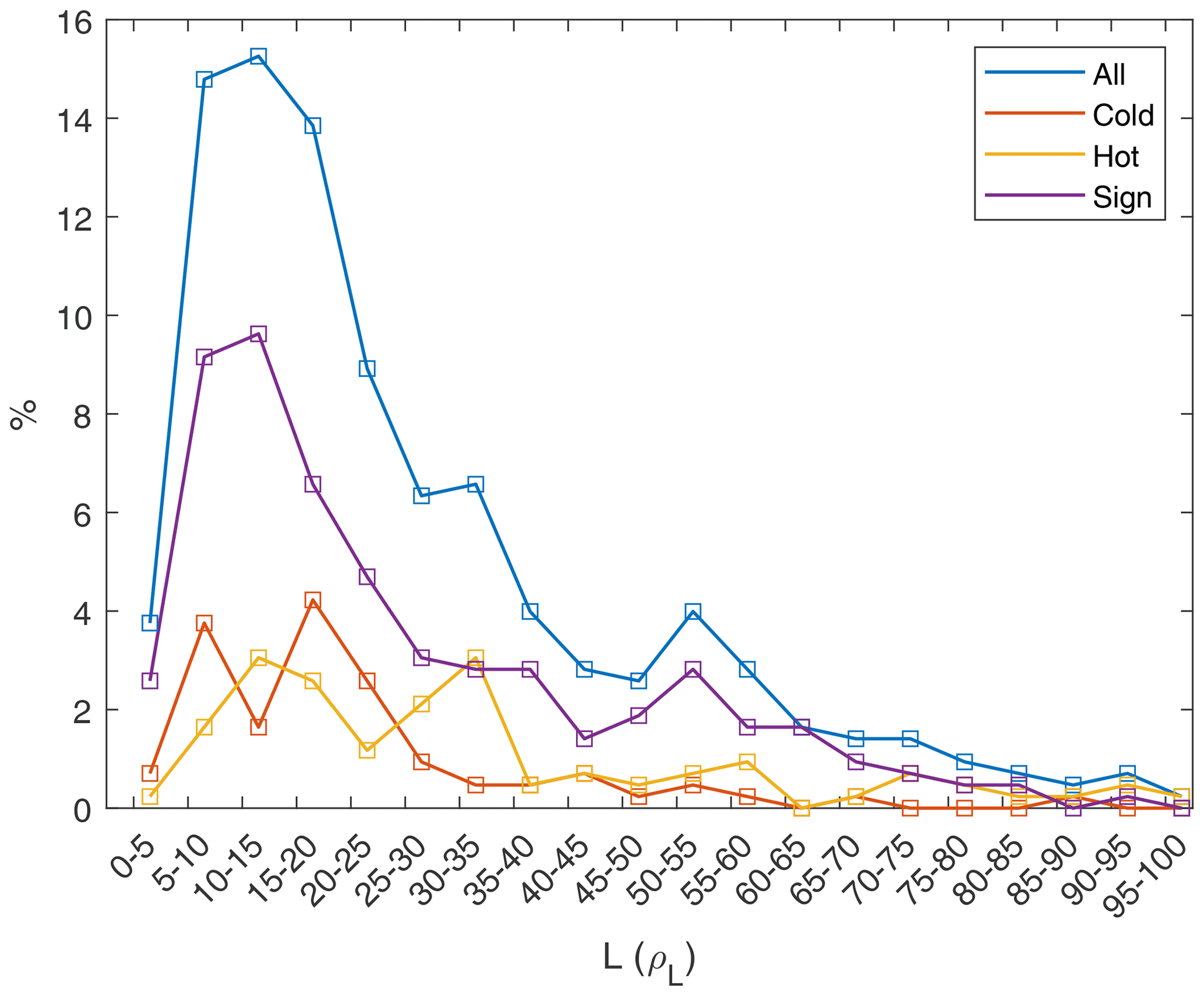
Of course, the width, w, of the structures measured in seconds does not say anything about the physical size of the structures and is mostly used when plasma parameters are not available for analysis. In the case of MMS the plasma data can be used to transform the width, w, into a physical size L. In Fig. 4 the size is given in units of the local proton thermal Larmor radii ρ_L:

$$\begin{array}{}\text{(4)}& L={\displaystyle \frac{w\cdot V_{\mathrm{SW}}}{{\mathit{\rho }}_{\mathrm{L}}}}={\displaystyle \frac{w{V}_{\mathrm{SW}}{q}_{\mathrm{p}}B}{\sqrt{\mathrm{2}{q}_{\mathrm{p}}{m}_{\mathrm{p}}{T}_{\mathrm{p}⟂}}}},\end{array}$$

where the perpendicular thermal velocity of the ions is calculated from the ion temperature ($v_{\text{th}⟂}=\sqrt{k_{\mathrm{B}}{T}_{\mathrm{p}⟂}/m_{\mathrm{p}}}$). The distribution for all events peaks in the bins $L=\mathrm{5}-\mathrm{20}{\mathit{\rho }}_{\mathrm{L}}$.

Figure 4 The distribution of the size L of the LMH structures in percentage of total events. The colour coding is the same as in Fig. 2.

3 Categorization

The identification of the LMH structures was done in the same way as in previous papers. The vicinity of the Earth and its bow shock could have an influence on the structures that are selected. Possibly, foreshock structures whose magnetic field signatures resemble a magnetic depletion like hot flow anomalies (e.g. Schwartz, 1995; Zhao et al., 2017), cavitons (Kajdič et al., 2013), cavities (Sibeck et al., 2002, 2004), density holes (Parks et al., 2006) or foreshock bubbles (Turner et al., 2020) can disturb the determination occurrence rate of MHs. Therefore, a categorization of these structures is made based on their magnetic and plasma characteristics, which will lead to three kinds of structures, discussed in the following subsections.

Figure 5 shows a scatter plot of all structures, described by $\mathrm{\Delta }N/N=(N_{\mathrm{in}}-N_{\mathrm{out}})/N_{\mathrm{out}}$ and $\mathrm{\Delta }T/T=(T_{\mathrm{in}}-T_{\mathrm{out}})/T_{\mathrm{out}}$ and colour-coded with $\mathrm{\Delta }B/B$. The figure shows that only a minority of the structures has $\mathrm{\Delta }N/N>\mathrm{0}$, whereas the majority of events has $\mathrm{\Delta }T/T>\mathrm{0}$. This means that pressure balance can be obtained in different ways: an increase in density or in temperature (or both). Noticeable is the almost empty upper right quadrant in the panels.

Figure 5 Scatter plot of the $\mathrm{\Delta }T/T$ vs. $\mathrm{\Delta }N/N$ for all LMH structures. The colour coding is the $\mathrm{\Delta }B/B$ of each structure.

Three categories are defined below which are visualized in Fig. 5b–d: cold ($\mathrm{\Delta }N/N>\mathrm{0}$), hot ($\mathrm{\Delta }N/N\le \mathrm{0},\mathrm{\Delta }T/T>\mathrm{0}$) and sign change (remaining cases, where one B component changes signs).

3.1 Cold LMH

The cold LMH is defined by a decrease in magnetic field strength and an increase in density, which leads to pressure balance over the structure, as shown in Fig. 5b. The structure in Fig. 1 is an example, and overall there are 75 structures that fall into this category. In Figs. 2, 3 and 4 these structures are represented by orange lines, which do not seem to have a distribution significantly different from the whole set of structures (blue lines).

Figure 1 shows an LMH with $\mathrm{\Delta }B/B\approx \mathrm{0.84}$. The electron density increases, albeit slightly shifted with respect to the centre of the hole, and the ion density remains almost constant in the hole. The oscillations that are seen in the ion density (as well as in the temperature and the velocity) at ∼20 s are caused by the spin tone of the spacecraft. The ion temperature shows that the parallel component T_i‖ increases in the middle of the hole, whereas the total ion temperature $T_{\mathrm{iT}}=(T_{\mathrm{i}⟂}+T_{\mathrm{i}\Vert })/\mathrm{2}$ only changes little. Before the hole in the solar wind, $T_{\mathrm{i}⟂}<T_{\mathrm{i}\Vert }$, whereas inside the hole and after the hole in the solar wind, $T_{\mathrm{i}⟂}>T_{\mathrm{i}\Vert }$. The electrons do not show any significant changes in temperature. The instability criterion R_SK shows that before the hole the solar wind plasma was MM-stable, whereas inside and after the hole, the plasma is MM-unstable.

Figure 6 Linear magnetic hole on 31 January 2018, category cold. Same format as in Fig. 1.

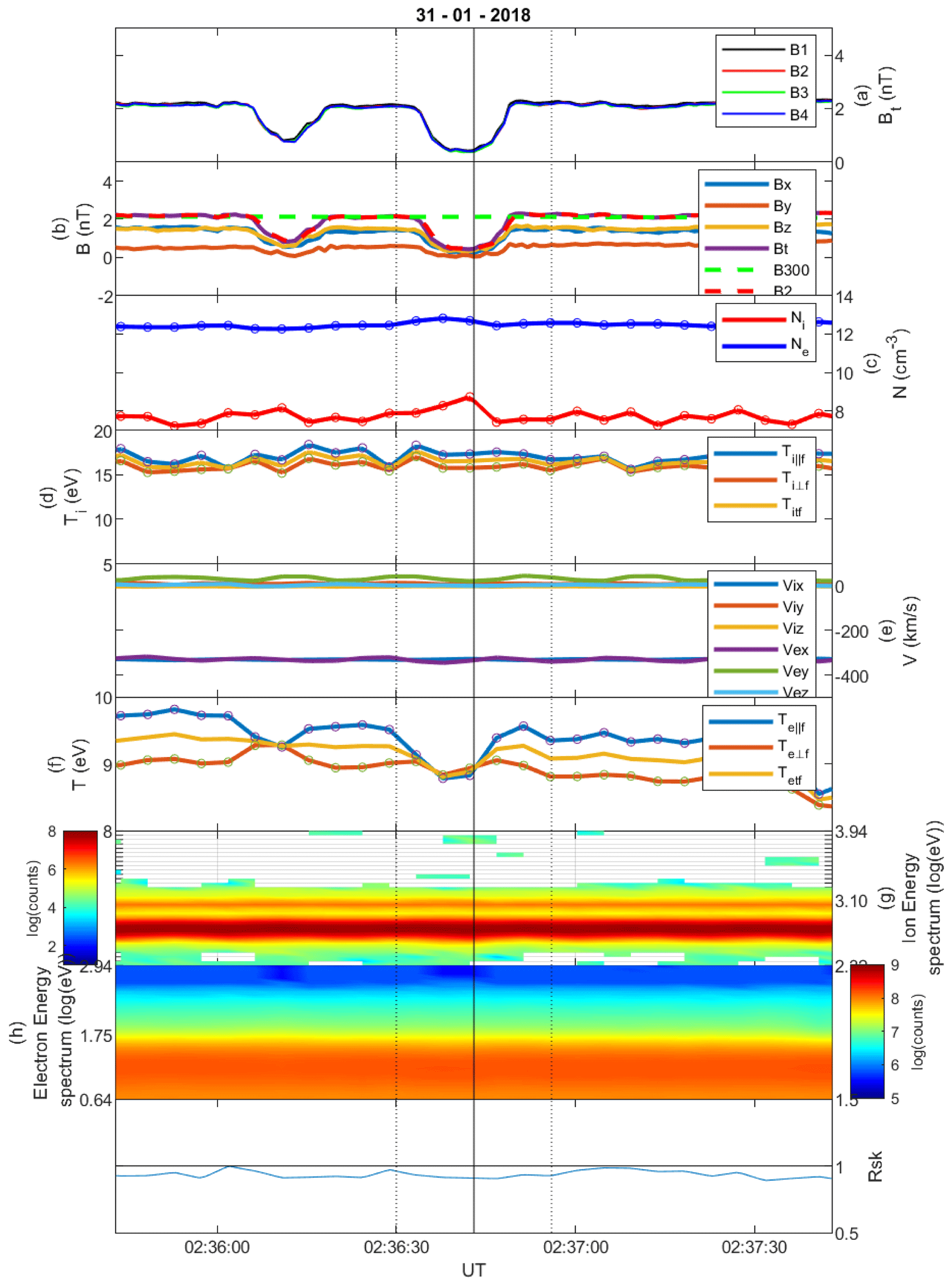
Figure 6 shows a very classical example of a LMH in the solar wind. There are actually two holes in this example, with the marked one being the deepest. Because of the selection criteria, the first one is not counted as an event, which will have influence on the occurrence rate of MHs, resulting in a 10 % difference in the total number of MHs (see Volwerk et al., 2020). The ion density data show an increase in density inside the holes of around 1 to 2 cm⁻³, whereas the electron density shows only little increase. The total ion temperature remains rather constant over the whole time interval in the figure, with $T_{\mathrm{i}\Vert }>T_{\mathrm{i}⟂}$, and R_SK<1, i.e. MM-stable. The total electron temperature $T_{\mathrm{et}}=(T_{\mathrm{e}⟂}+T_{\mathrm{i}\Vert })/\mathrm{2}$ slightly decreases in the central hole, and in both holes $T_{\mathrm{e}\Vert }\approx T_{\mathrm{e}⟂}$, but T_e‖ decreases in both holes.

3.2 Hot LMH

The hot LMH is defined by a decrease in density inside the hole (or a very small increase) and a strong increase in temperature (Fig. 5c). An example of a hot LMH is shown in Fig. 7. Once again there is a decrease of the magnetic field strength with $\mathrm{\Delta }B/B\approx \mathrm{0.61}$ with very little density variation but a strong increase in T_i⟂. The hole is embedded in a MM-stable plasma, with R_SK<1; only in the left part of the event window does it show a value >1, where $T_{\mathrm{i}⟂}>T_{\mathrm{i}\Vert }$. Also interesting is the “double dipped” magnetic structure, which could be an indication of the merging of two holes, which will be addressed in the Discussion section.

Figure 7 Linear magnetic hole on 17 December 2017, category hot. Format as in Fig. 1.

In total there are 94 structures in this category, which are shown by yellow lines in Figs. 2, 3 and 4. They approximately follow the same distribution as the full set in Fig. 2. However, looking at their sizes in Figs. 3 and 4, the distribution looks slightly broader than for the other categories, up to L=35ρ_L.

Figure 8 Linear magnetic hole on 23 February 2018, category hot. Format as in Fig. 1.

In Fig. 8 another example of a hot hole is shown. The decrease in B is combined with a constant density and an increase in temperature T_it, mainly created by an increase in T_i⟂. Overall, the perpendicular ion temperature remains greater than the parallel ion temperature and R_SK>1, so the region and the structures are MM-unstable until after the second dotted line. Only ∼30 s after the LMH does the plasma become MM-stable after an abrupt change in the IMF direction, a rotation from B_y into B_z. The electrons show a decrease in T_e‖ inside the hole.

3.3 Sign change LMH

After the definition of the cold and hot categories of LMHs, there is still a large group of events that is left. These all have the characteristic that (at least) one of the magnetic field components change sign over the structure. There are a total of 237 structures in this category, i.e. the majority. They show up both in the cold and hot quadrants in Fig. 5d; 43 are cold, 155 are hot, and 39 are in the region where both the density and temperature decrease.

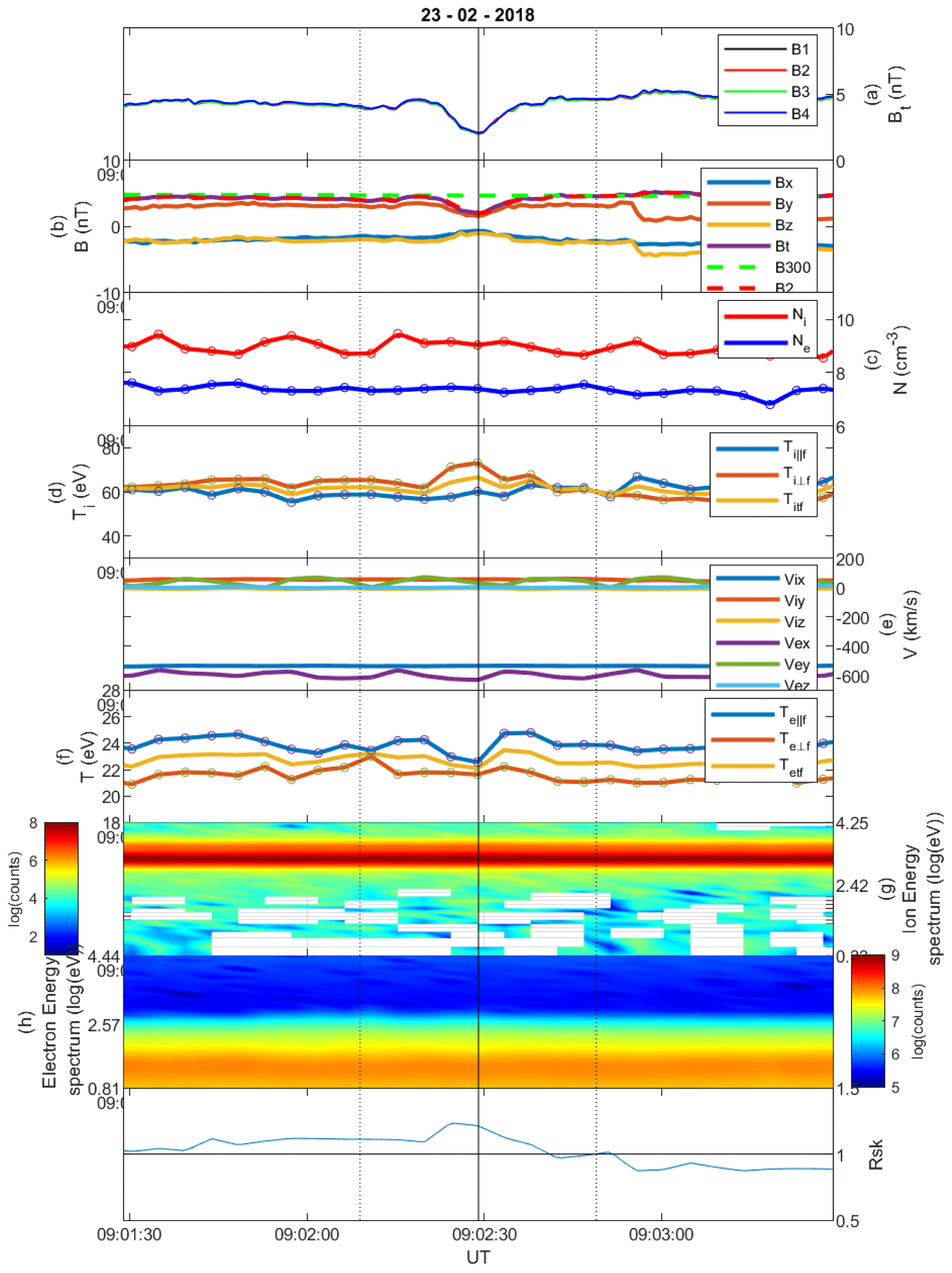
An example is shown in Fig. 9, and, although there is a sign change, the rotation of the field over the hole is still less than 10^∘. There is an increase in the ion temperature over the structure, but the parallel electron temperature decreases, and the density remains constant. Just outside the hole, the ion temperature drops, and the electron temperature and density increase.

There is possibly an additional MH at the beginning of the interval shown in Fig. 9, where at ∼ 04:10:10 UT, there is an increase in ion and electron density, and T_i⟂ drops to be equal with T_i‖, but T_e⟂ increases slightly.

The solar wind is strongly deflected by $\sim \mathrm{45}{}^{\circ }$ in the XY_GSE direction. The ion energy spectrum is very broad, indicating that this event is most likely in the Earth's magnetosheath.

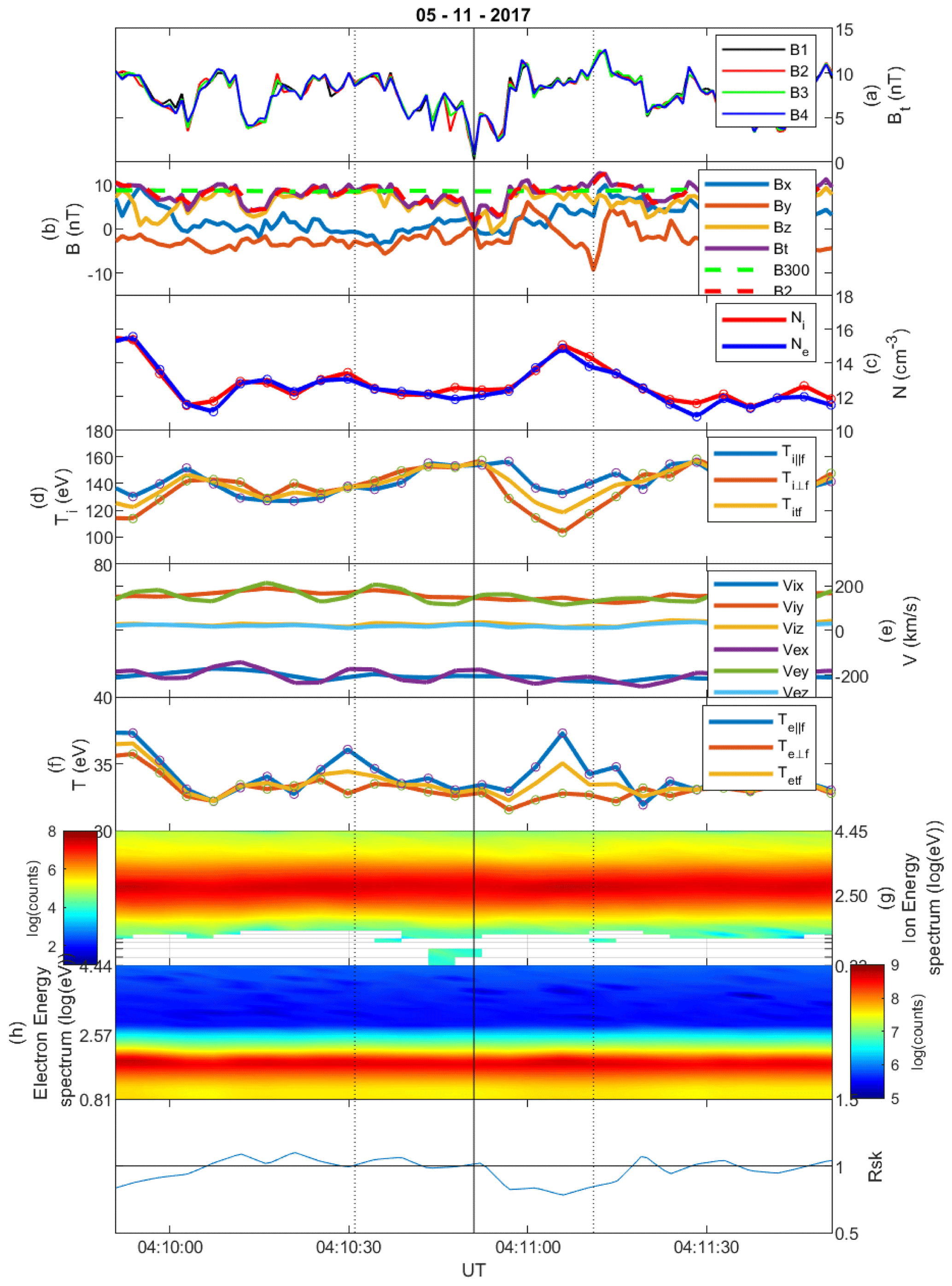
Figure 9 Linear magnetic hole structure on 5 November 2017, category sign change. Format as in Fig. 1.

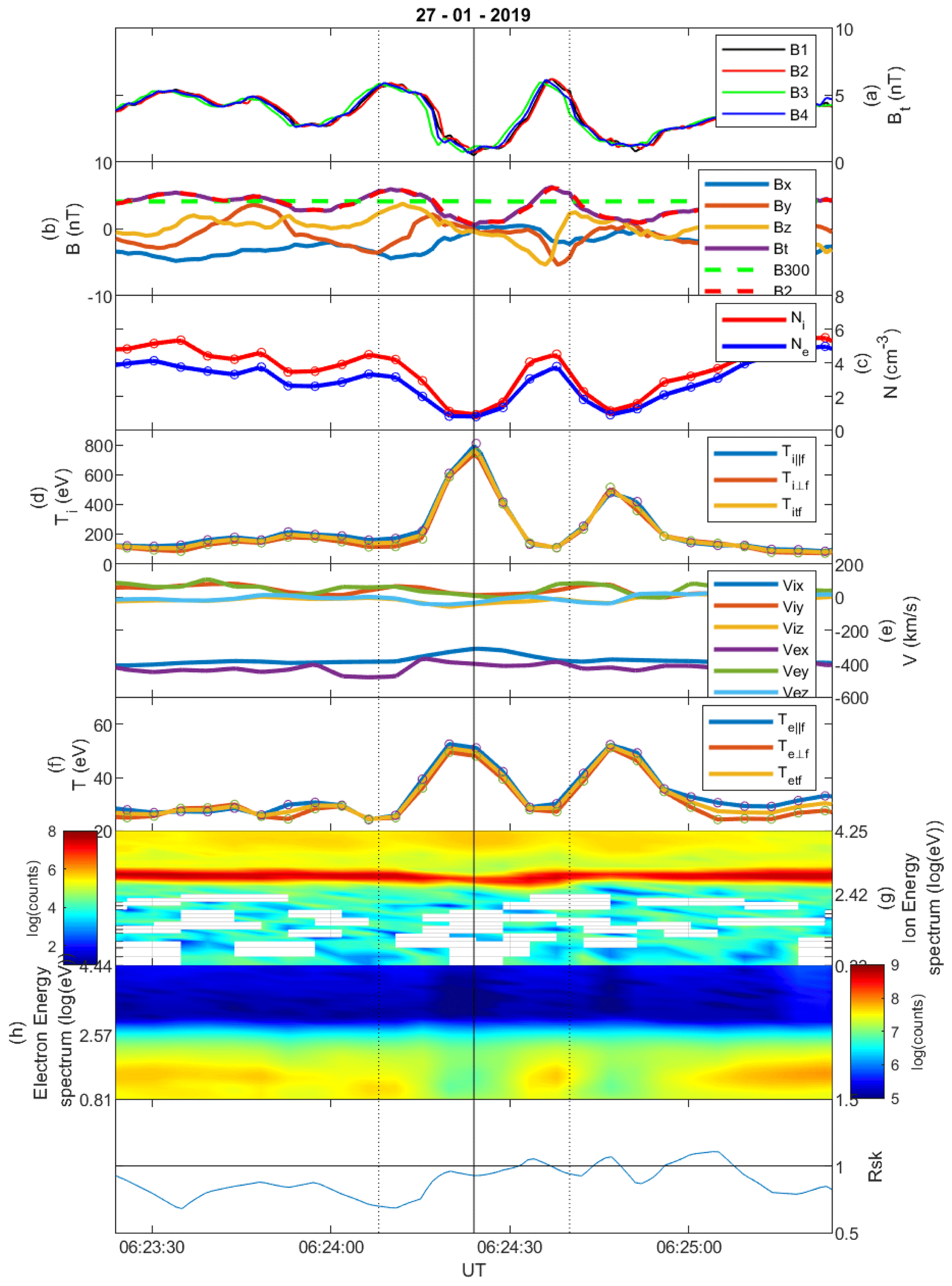
Figure 10 Linear magnetic hole on 27 January 2019, category sign change. Format as in Fig. 1.

Figure 10 shows another example of a sign change LMH, where clearly B_y and B_z change signs over the width of the hole. The ion and electron density drop drastically, and the ion and electron temperature increase drastically. The solar wind is not deflected, as in the previous case, but the ion energy spectrum shows very hot ions above the narrow solar wind ions, indicating that this structure is also in the Earth's foreshock.

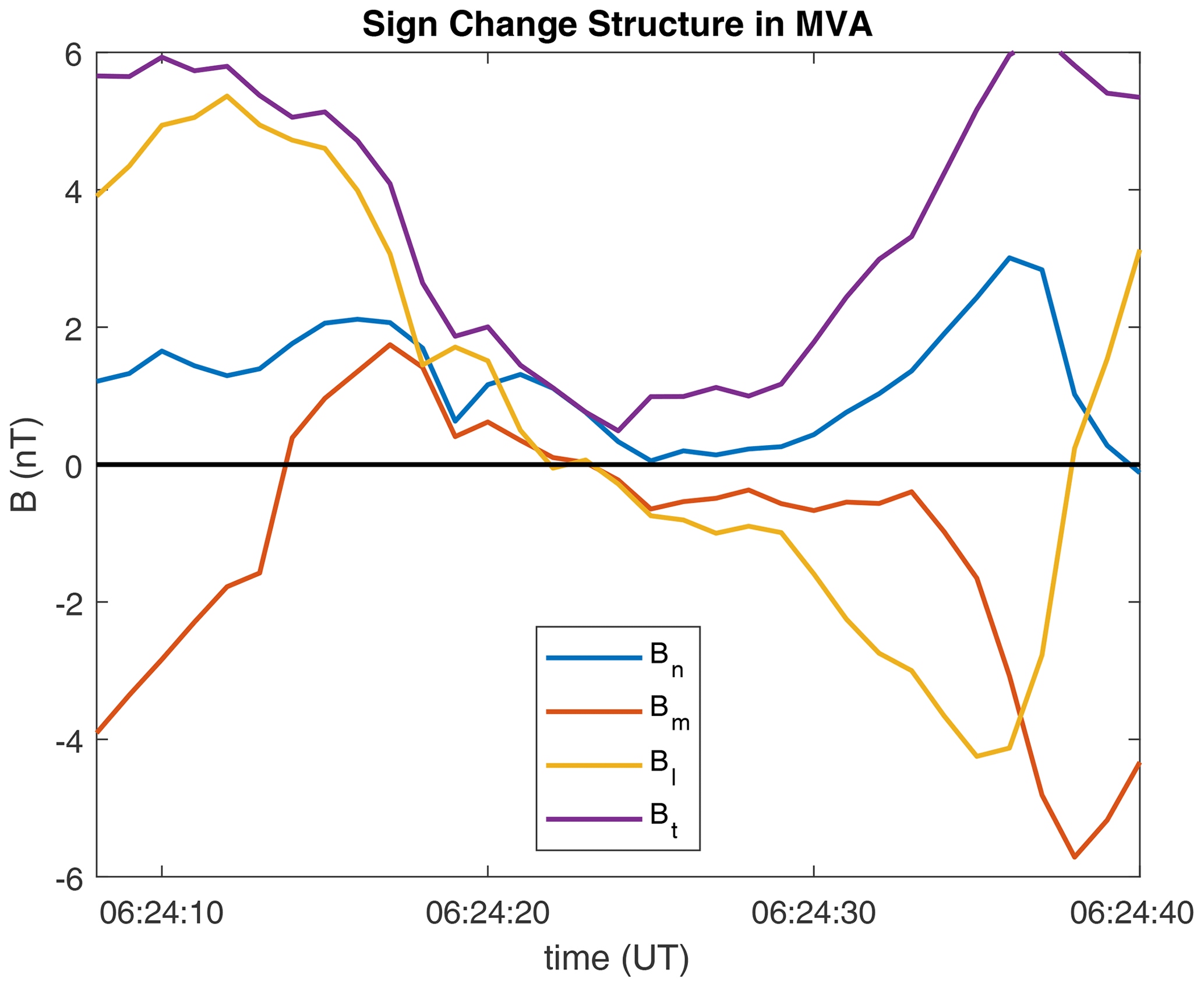
For the structure shown in Fig. 10 a minimum variance analysis (MVA; Sonnerup and Scheible, 1998) was performed on the interval between the two vertical dotted lines in panel (a), and the magnetic field data were transformed into the lmn system (with l for maximum, m for intermediate and n for minimum variance directions), shown in Fig. 11. The ratio of the intermediate-to-minimum eigenvalue is ${\mathit{\lambda }}_{\mathrm{int}}/{\mathit{\lambda }}_{\min }\approx \mathrm{5.9}$, whereas that of the maximum-to-intermediate eigenvalue is ${\mathit{\lambda }}_{\max }/{\mathit{\lambda }}_{\mathrm{int}}\approx \mathrm{2.3}$, which means that the MVA is well determined (Sergeev et al., 2006). Between the two maxima in B_t (purple), the B_n component (blue) remains almost constant, B_m (yellow) decreases strongly towards values around 0 nT and B_l shows a sign change from ∼5 to $\sim -\mathrm{4}$ nT. The l direction is $[-\mathrm{0.52},\mathrm{0.0},\mathrm{0.8}]$, mainly in the Z_gse direction, and the location of the spacecraft is $[\mathrm{20.6},\mathrm{2.3},\mathrm{6.5}]R_{\mathrm{E}}$. This behaviour may be consistent with the signature of a flux rope passing over the spacecraft or of a hot flow anomaly (see, for example, Schwartz et al., 2018).

Figure 11 Sign change hole of Fig. 10 transformed into an MVA coordinate system.

4 Pressure balance

As discussed in the Introduction, these LMH structures are assumed to be in pressure balance with their surroundings (Burlaga and Lemaire, 1978; Burlaga et al., 1990; Winterhalter et al., 1995). The decrease in magnetic pressure needs to be balanced by an increase in plasma pressure, which means a density or temperature increase.

In order to study the pressure balance of these structures, the magnetic pressure and the plasma pressure are calculated: inside at the centre of the structure and outside the average over two intervals of 30 s before and after the structure is calculated, similar to the determination of the magnetic field outside the LMHs. In Fig. 12a the relation between the total pressure outside and inside is presented by green circles. The black line shows the identity, on which the points should lie for perfect pressure balance and perfect instrumentation. The red line shows a linear fit to the green points, with the regression coefficient and the slope listed in the figure. It is clear that there is a spread in the points around the identity. Figure 12b–d show the relations for the different categories, cold, hot and sign change, respectively.

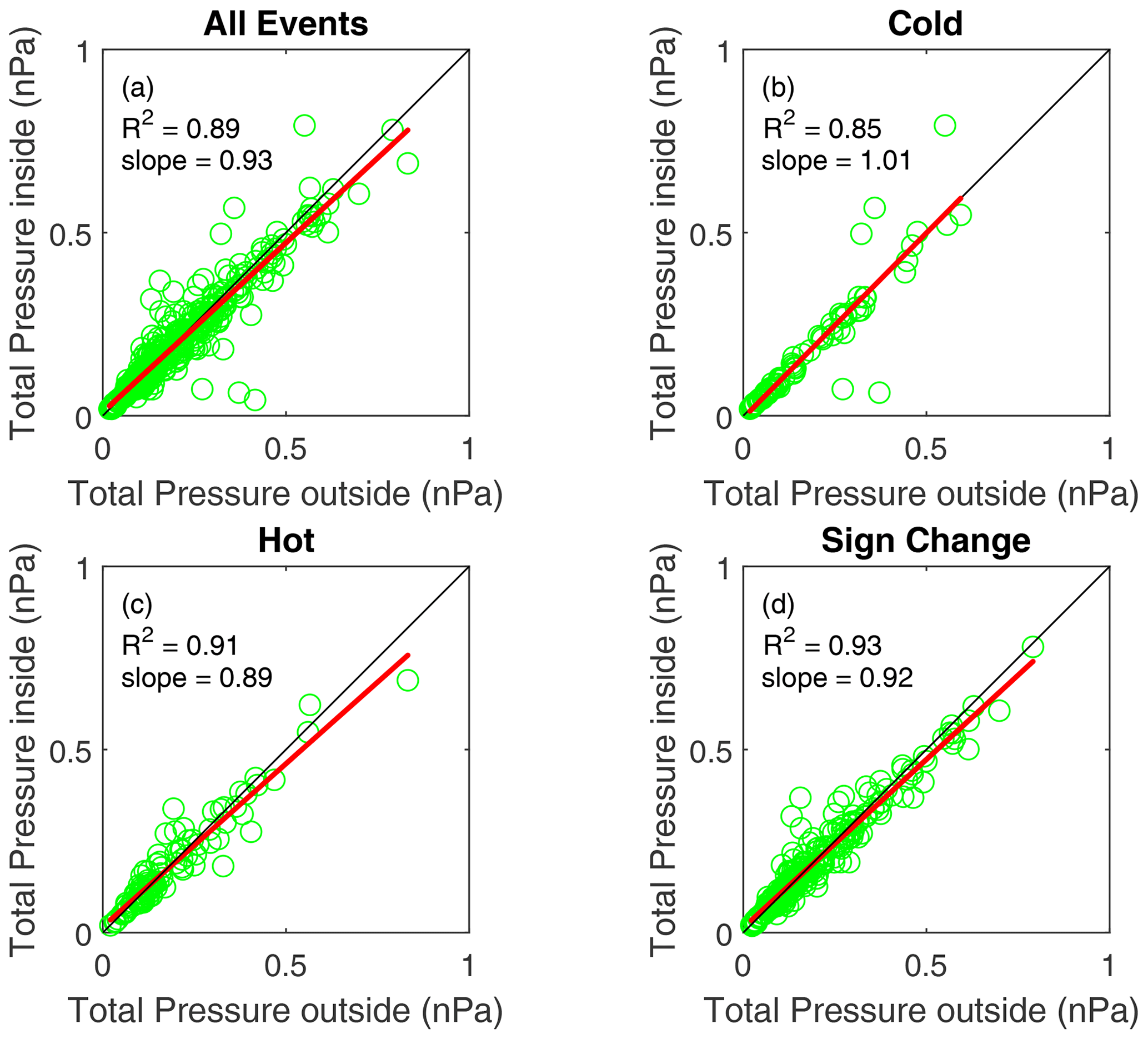
Figure 12 Test of the pressure balance over the structures. The total pressure is calculated at the centre and outside of the structure. (a) Relation for all structures; the black line is the identity, and the red line is a fit to the points. Pressure balances follow for (b) the cold category, (c) the hot category and (d) the sign change category. The regression coefficients and the slopes are listed in the panels.

The cold LMHs show that, apart from five structures, there is almost perfect pressure balance, demonstrated by the slope of 1.01 of the linear fit to the points. The five exceptions, three above and two below the identity, are influenced by hot ions in the foreshock region. For the hot and sign change LMHs, the spread around the identity is larger, and the slope of the fit deviates more from the identity.

5 Categories revisited

Three categories of MHs are defined above; however, this alone does not clear up the differences between them, e.g. how and where each category is created. For the sign change LMHs it was determined that these are mainly foreshock structures. Figure 13 shows, for each category, the location of the structures and the direction of average background magnetic field projected onto the XY plane.

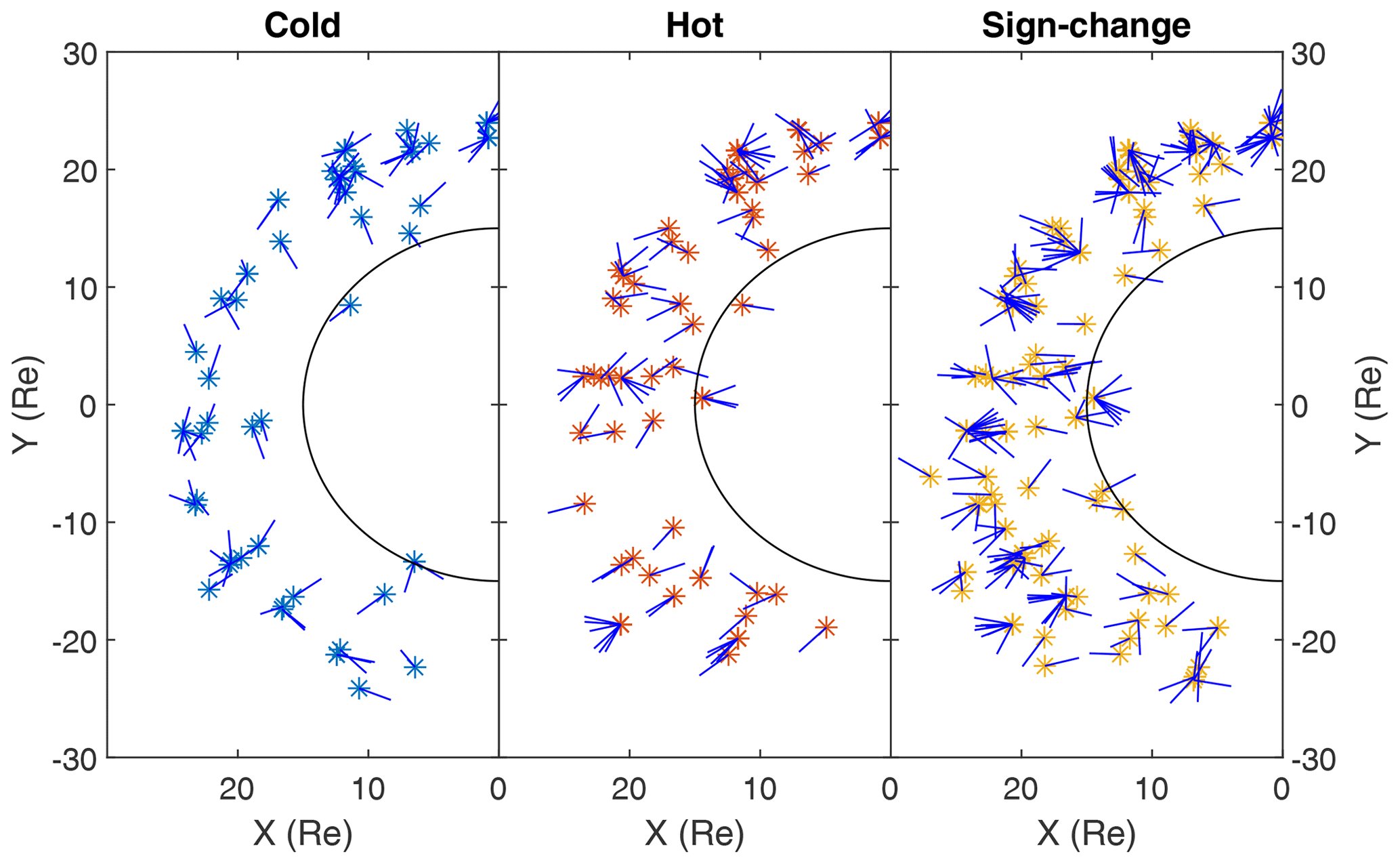
Figure 13 Location of the events in the GSE XY plane with the average magnetic field direction for the three categories. The black circle represents the 15R_E boundary outside of which the LMHs are searched for.

In order to find out if the events are connected to the bow shock, the angle between the magnetic field direction and the radial direction to the spacecraft is calculated. Figure 14 shows the percentage of events in bins of 10^∘ between the radial direction and the magnetic field direction. (Note that the angles are folded around 90^∘ as the magnetic field can point in two directions.)

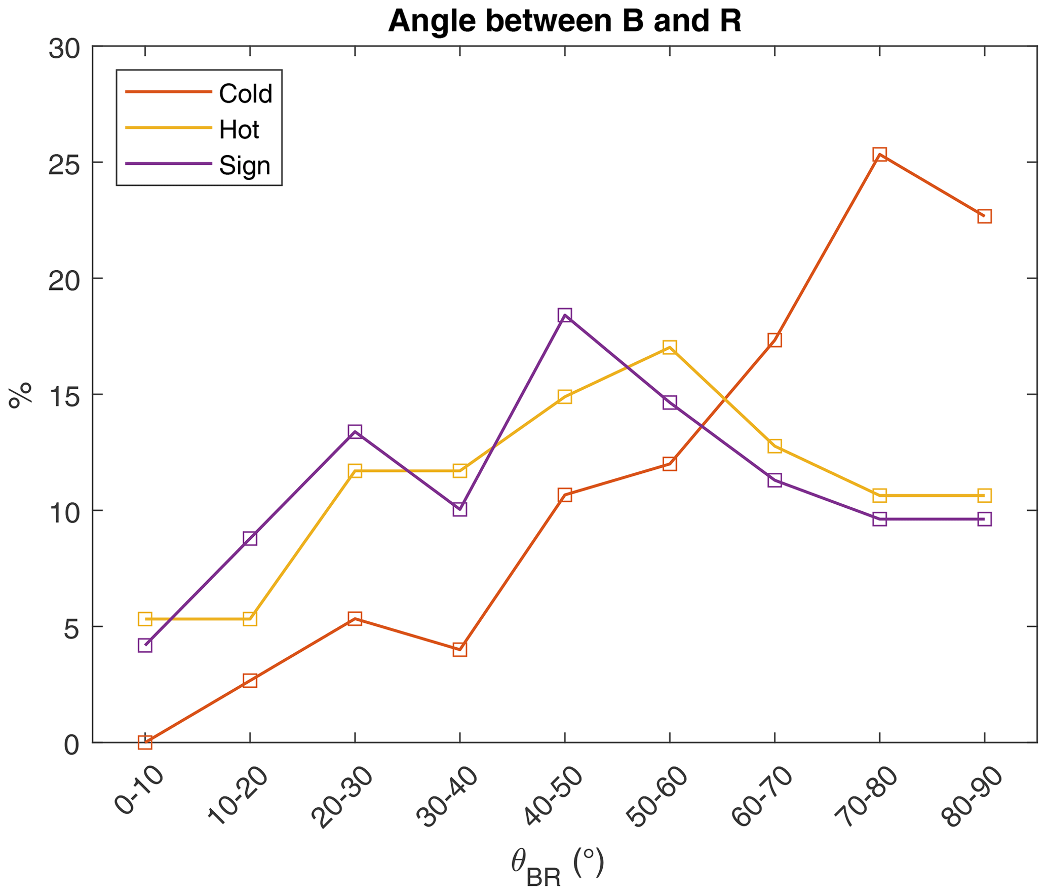
Figure 14 The angle between the radial direction and magnetic field direction binned per category in 10^∘-wide bins as a percentage of the total number of structures per category.

Figure 14 shows that for the cold LMHs the distribution increases strongly for larger angles. With ∼20 % events with an angle ${\mathit{\theta }}_{\mathrm{BR}}\le \mathrm{50}{}^{\circ }$, it can be concluded that these structures have basically no connection to the bow shock; i.e. they are not influenced by the foreshock region.

For the hot and sign change LMHs, there is basically the same distribution of angles, with ∼50 % events with an angle ${\mathit{\theta }}_{\mathrm{BR}}\le \mathrm{50}{}^{\circ }$, indicating that a much greater part of these structures can have a connection to the bow shock and can be influenced by foreshock processes.

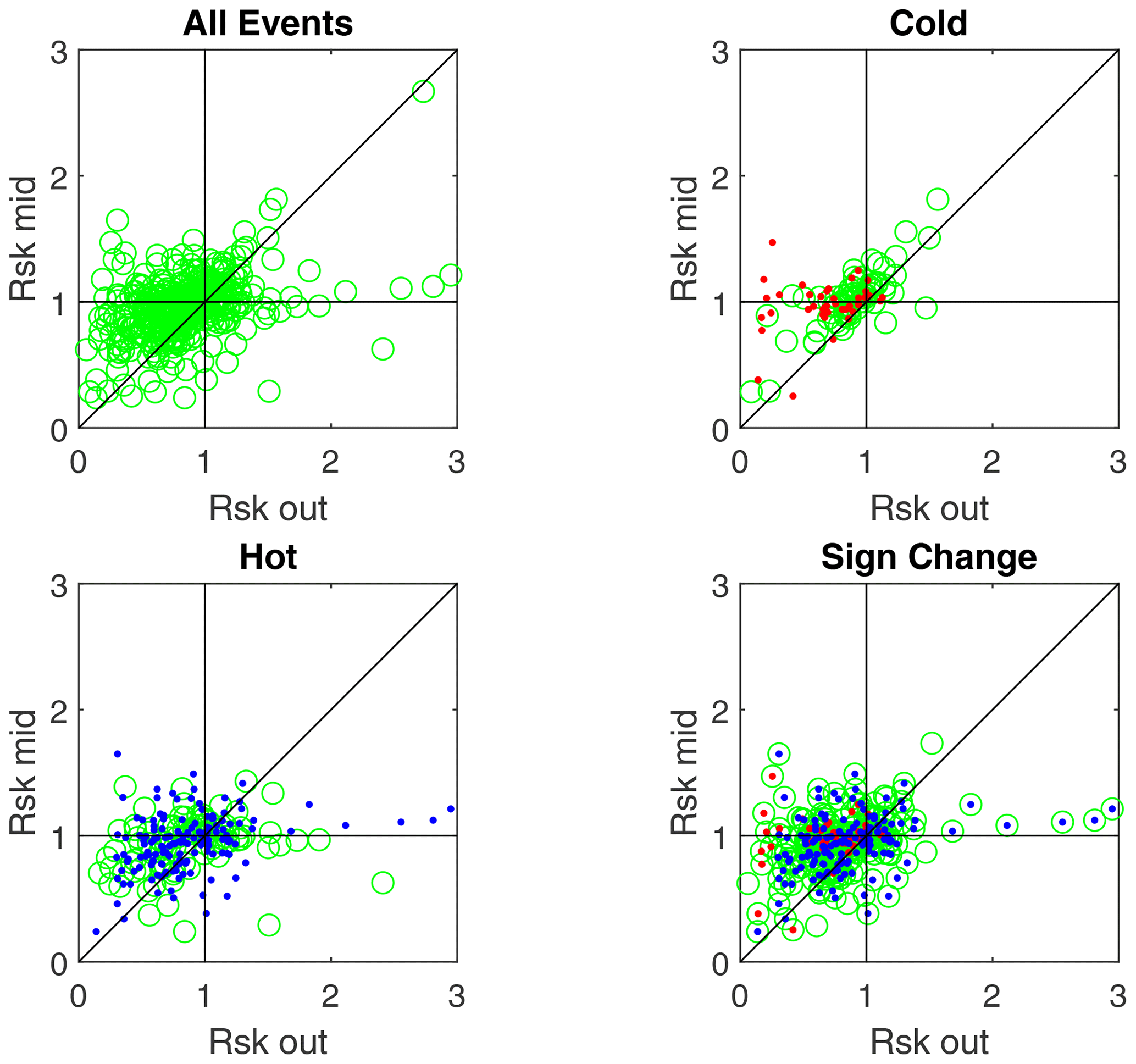
Figure 15 The MM instability criterion of Eq. (1), R_SK, inside the LMH vs. outside. The full list of structures and the three categories are shown. The horizontal and vertical black lines show where R_SK=1, and the diagonal black line is the identity. The red (43) and blue (155) dots are the cold and hot LMHs in the sign change category.

As it is often suspected that MHs are the final stage of MMs, the instability criterion R_SK (Eq. 1) is determined inside and outside of the structures. Outside, the mean value over 30 s before and after the structure is determined (similar to the average magnetic field), and inside, the value at the centre of the LMH is used. The criterion R_SK in the middle of the structure vs. outside of it is plotted in Fig. 15. The cold (43) and hot (155) LMHs for the sign change category have also been determined and plotted as red and blue dots respectively, both of them in the sign change panel, and per category in the cold and hot panels. This shows that most of the cold–sign change LMHs occur for $R_{\mathrm{SK},\mathrm{out}}<\mathrm{1}$; the hot–sign change LMHs form a cloud similar to the green circles.

For the plasma to be MM-unstable it is required that R_SK>1. It is clear from Fig. 15 that there is a large group of structures that lie beyond the line R_SK=1 on both axes. The percentages of stable LMHs are given in Table 2.

A note should be made here about the instability criterion R_SK>1, which depends on the ion density and temperature; see Eqs. (1) and (2). Because of the observed discrepancies between the ion data from FPI and the Wind mission (Bandyopadhyay et al., 2020) or OMNI (Roberts et al., 2021), one should be cautious in interpreting the results shown in Fig. 15 and in Table 2.

Table 2 Top: numbers and percentages of MM-stable conditions outside and inside of the LMHs per category. Bottom: numbers and percentages of MM-stable LMHs in stable outside plasma and of MM-stable LMHs in unstable outside plasma.

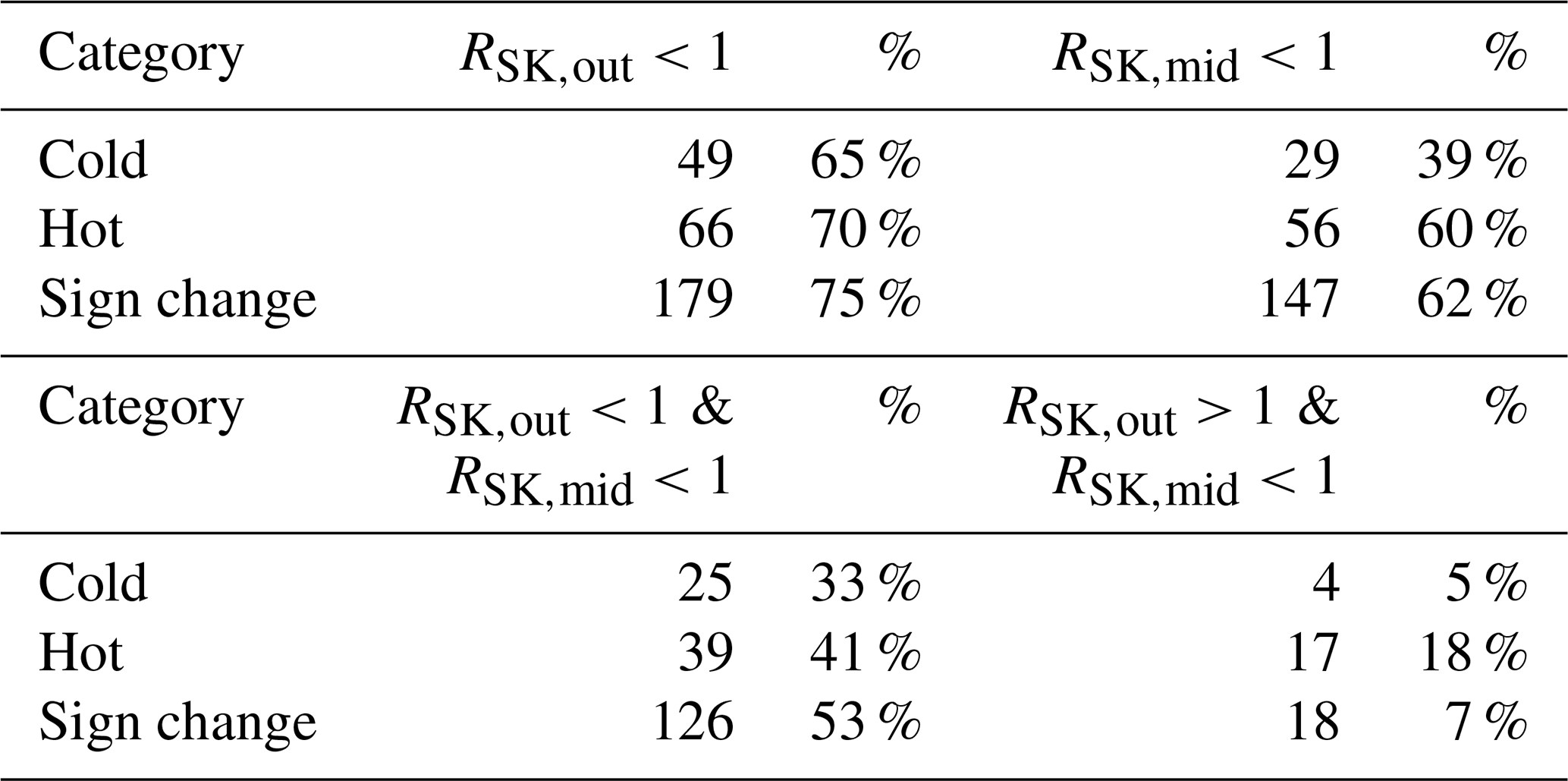
The percentages shown in Table 2 for LMHs embedded in MM-stable plasma and MM stability inside the LMHs are quite low, something that was also found by Madanian et al. (2020) using MAVEN data in the solar wind upstream of Mars.

6 Discussion and conclusions

The characteristics of the ubiquitous magnetic hole structures, that are indicative of temperature asymmetries in space plasmas, were studied just outside the Earth's bow shock (R≥15R_E) with the MMS1 spacecraft. Naturally, due to the dynamics of the bow shock (see, for example, Meziane et al., 2014) 15R_E may not suffice in some cases, which will then be magnetosheath structures. A test has been performed on the closest bin, 15−16R_E, to see how many of the 22 events were in the magnetosheath, which resulted in only three events, all on the same day.

Because of the large size of the MHs in the solar wind and the small inter-spacecraft distance, only the data from one MMS spacecraft are analysed. Figure 1a and consecutive data figures show how little difference exists between the magnetic field data. This also means that the usual four-spacecraft analysis methods, such as timing and curlometer techniques (Schwartz, 1998), cannot be applied here. Only a significant difference between the spacecraft can be observed in the case of sub-ion magnetic holes (Wang et al., 2020c, b). A set of 406 structures were found with $\mathrm{\Delta }B/B>\mathrm{0.5}$ and a maximum rotation of the magnetic field of $\mathrm{\Delta }\mathit{\theta }\le \mathrm{10}{}^{\circ }$, over a time span of 8 months in 2017 and 2018. This leads to an initial occurrence rate of 2.3 per day, which is slightly higher than earlier presented rates.

After inspection of the combined magnetic field and plasma data, the LMH structures were split up into three categories:

• cold LMHs, characterized by a decrease of the magnetic field strength, combined with an increase in density which ensures pressure balance over the structure (75 structures);

• hot LMHs, characterized by a decrease of the magnetic field strength, combined with an increase in temperature with little density variation (94 structures);

• sign change LMHs, characterized by a decrease of the magnetic field strength, combined with the change of sign of at least one of the magnetic field components (237 structures, of which 43 are cold and 155 are hot).

If only the first two categories are counted as LMHs, as the sign change might be foreshock structures, then the occurrence rate listed in Table 1 should be reduced by a factor of 0.4, leading to a rate of 0.9 per day. This would be lower than what has been observed near Earth in previous studies as listed in Table 1. Using Cluster data, Xiao et al. (2014) showed in their Table 1 occurrence rates of 0.8 and 1.1 per day for 2003 and 2004, which were also years during the declining phase of the solar cycle, in the same way as 2017 and 2018 for the present study with MMS. Also, the conditions for LMHs that Xiao et al. (2014) used ($B_{\min }/B\le \mathrm{0.75}$ and less than 15^∘ rotation of the field over the LMH) are less stringent than in this paper.

Figure 5 shows that the density variation seems to be limited to $-\mathrm{1}<\mathrm{\Delta }N/N=(N_{\mathrm{in}}-N_{\mathrm{out}})/N_{\mathrm{out}}<\mathrm{1}$. This means that the limit on the density inside, for the structures in this study, is N_in<2N_out. Similarly the temperature is limited $\mathrm{\Delta }T/T=(T_{\mathrm{in}}-T_{\mathrm{out}})/T_{\mathrm{out}}>-\mathrm{1}$, but there should be no real upper limit. For the cases in this study, T_in<6T_out. These specific limiting values are, most likely, the result of the pressure balance of these structures, as shown in Fig. 12.

One main result is that the structures are all basically in pressure balance with their surroundings, as is clearly shown in Fig. 12. This was also found by Madanian et al. (2020) for some events in Mars's extended exosphere, where the ion temperature increased, and these events would thus fall into the hot category of this paper.

Another main result concerns the MM instability criterion; i.e. R_SK>1. In this study only ∼54 % of all structures, though varying by category, have $R_{\mathrm{SK},\mathrm{mid}}<\mathrm{1}$ and thus are MM-stable. Winterhalter et al. (1995) found that the MHs mainly occurred in a (marginally) stable plasma environment. In this study ∼70 % of the structures are embedded in an MM-stable plasma environment, $R_{\mathrm{SK},\mathrm{out}}<\mathrm{1}$, and ∼10 % of the structures in an MM-stable environment are MM-unstable inside.

Would one not expect stability inside the structure if the MHs are the final stage of MMs, for which the instability criterion should have been relaxed through the creation of the MMs? One reason for a temperature asymmetry in the MHs is the presence of an ion or electron vortex in the MH, the presence of which was shown by Wang et al. (2020b, a). Why less than half of the structures are still (or again) MM-unstable needs to be further investigated, e.g. by numerical simulations, to find the temporal evolution of MHs. A dedicated ISSI team on the topic “Towards a unifying model for magnetic depressions in space plasmas” will study this topic further.