the Creative Commons Attribution 4.0 License.
the Creative Commons Attribution 4.0 License.
 | 10 Jun 2024
On the importance of middle-atmosphere observations on ionospheric dynamics using WACCM-X and SAMI3
Fabrizio Sassi
Angeline G. Burrell
Sarah E. McDonald
Jennifer L. Tate
John P. McCormack
Recent advances in atmospheric observations and modeling have enabled the investigation of thermosphere–ionosphere interactions as a whole-atmosphere problem. This study examines how dynamical variability in the middle atmosphere (MA) affects intra-day changes in the thermosphere and ionosphere. Specifically, this study investigates ionosphere–thermosphere interactions during different time periods of January 2013 using the Specified Dynamics Whole Atmosphere Community Climate Model, eXtended version (SD-WACCM-X), coupled to the Naval Research Laboratory (NRL) ionosphere of the Sami3 is Another Model of the Ionosphere (SAMI3) model. To represent the weather of the day, the coupled thermosphere–ionosphere system is nudged below 90 km toward the atmospheric specifications provided by the Navy Global Environmental Model for High-Altitude (NAVGEM-HA). Hindcast simulations during January 2013 are carried out with the full dataset of observations normally assimilated by NAVGEM-HA and with a degraded dataset where observations above 40 km are not assimilated. Ionospheric regions with statistically significant changes are identified using key ionospheric properties, including the electron density, peak electron density, and height of the peak electron density. Ionospheric changes show a spatial structure that illustrates the impact of two different types of coupling between the thermosphere and the ionosphere: variability induced by wind-dynamo coupling through electric conductivity and ion-neutral interactions in the upper thermosphere. The two simulations presented in this study show that changing the state of the MA affects ionosphere–thermosphere coupling through changes in the behavior and amplitude of non-migrating tides, resulting in improved key ionospheric specifications.
- Article
(2357 KB) - Full-text XML
- BibTeX
- EndNote


The development of whole-atmosphere models (ground to exobase) in the last decade along with the availability of high-altitude atmospheric data assimilation has brought the geospace community closer to important understandings of the prediction of short-term variability (≤10 d) in the lower E region. When the Sun is quiescent, a large fraction of the short-term variability in the E region is driven by lower-atmosphere weather from below. Because of wind-dynamo coupling in this region, neutral variability affects the state of the ionosphere both locally and at higher altitudes.
The impact of atmospheric weather on the behavior of the coupled thermosphere–ionosphere system is a topic that has been actively investigated for nearly a century. From small-scale gravity waves (Hines, 1960) to planetary-scale waves (Forbes and Zhang, 1997), meteorological weather impacts the ionosphere either through electrodynamics (e.g., E×B drifts) or collisional interactions whose impacts greatly affect ion transport along field lines. Forbes et al. (2000) show that the fraction of ionospheric variability (obtained from the critical frequency at the F peak, foF2) due to meteorological conditions depends on the period of the meteorological forcing itself and varies between 20 % and 35 % with respect to the long-term mean (calculated using data from 1967–1989) during solar minimum conditions; modeling studies tend to estimate a higher fraction for the meteorological contribution, approaching 50 % (e.g., Liu et al., 2013). The role of migrating and non-migrating tides in determining the variability and structure of the ionosphere on many timescales, from days to seasons, is prominent and well established (Hagan et al., 2007; Liu, 2016; Sassi et al., 2019 and references therein). Migrating solar tides are associated with a modulation of the daily variability of vertical ion drifts at the geomagnetic equator (Millward et al., 2001; Fang et al., 2013). In particular, the migrating semidiurnal solar tide has been associated with a shift of meridional ion drifts (which are directed vertically at the geomagnetic equator), and consequently of the peak electron density, to earlier local times during days immediately following a sudden stratospheric warming (SSW) (e.g., Goncharenko et al., 2010; McDonald et al., 2015; Fuller‐Rowell et al., 2017). When studied at a fixed local time (LT), non-migrating tides have instead been associated with the zonal structure of the ionosphere (Forbes et al., 2008; Immel et al., 2006) and have been found to be very sensitive to the background meteorological conditions of the lower atmosphere (McDonald et al., 2018; Sassi et al., 2020). In addition to solar tides, lunar tides are known to be impactful on the field-aligned neutral winds that help shape the structure of the F-peak ionosphere (Pedatella and Maute, 2015). Furthermore, a statistical analysis that aggregates the response of the equatorial ionization anomaly (EIA) over many SSWs (Wu et al., 2021) shows that the timing of the modulation of the EIA following an SSW is affected by the lunar phase.
Such theoretical progress in understanding the coupling between the thermosphere and the ionosphere has, in part, been possible because of momentous advances in the development of whole-atmosphere numerical models during the last decades that also include electrodynamic interactions (e.g., Liu et al., 2010, 2018). At the same time, the development of these modeling capabilities has benefited from the availability and utilization of observations well into the upper atmosphere and the extension of forecast/assimilation systems that provide specifications in the upper atmosphere (Eckermann et al., 2009; Wang et al., 2011; McCormack et al., 2017; Eckermann et al., 2018). Thus, investigations of the Coupled Ionosphere Thermosphere System (CITS) have been guided and validated by observations (Jin et al., 2012), both through nudging techniques (e.g., Sassi et al., 2013) and full data assimilation (Wang et al., 2011; Pedatella et al., 2018). In most cases, the need for upper atmospheric observations is not limited to merely validating forecast and hindcast simulations but rather extends to fundamental advances in theoretical understanding of whole-atmosphere interactions (Liu, 2016; Sassi et al., 2019, for reviews). Observations are critical to evaluate and improve predictions in the whole atmosphere: Liu et al. (2009) demonstrated that the troposphere plays a critical role in controlling error growth at higher altitudes. Pedatella et al. (2013) used a data assimilation system to reduce the global root mean square error in zonal wind up to 40 % in the upper mesosphere and lower thermosphere (UMLT), and in a later study, Pedatella et al. (2019) used a whole-atmosphere model with a data assimilation system to demonstrate that the error growth in the lower thermosphere saturates within 5 d.
Observations of the middle atmosphere (MA), which consists of both the stratosphere and mesosphere, are primarily obtained from instruments carried on board spaceborne platforms. Unfortunately, many research platforms have surpassed their expected lifetime, such as the Sounding of the Atmosphere using Broadband Emission Radiometry (SABER) instrument on board the NASA Thermosphere Ionosphere Mesosphere Energetic Dynamics (TIMED) satellite, while critical operational platforms are not being replaced (e.g., the Defense Meteorological Satellite Program (DMSP)) (e.g., Erwin and Berger, 2021). As noted by Sassi et al. (2020), the potential lack of observations in the MA has significant implications for capturing intra-day variability of neutral winds in the lower thermosphere. In particular, the amplitude of some non-migrating solar tides and of traveling planetary-scale waves can change by a factor of 2 during boreal winter. It stands to reason that such prominent changes of the thermospheric weather will have consequences for the structure and variability of the ionosphere. To the best of our knowledge, the fundamental question of how numerical simulations of physical properties of the CITS are impacted by data loss in the middle atmosphere remains elusive and poorly described.
This study seeks to answer the fundamental question of whether the loss of MA observations is potentially consequential for predictions of thermosphere–ionosphere coupling. In Sect. 2, the different models used in this study are presented, and details about the run configurations are provided. Section 3 presents the results of the model runs, Sect. 4 presents a discussion of the results, and Sect. 5 presents the conclusions.
Three models are used in this study: the Navy Global Environmental Model for High-Altitude (NAVGEM-HA), the Whole Atmosphere Community Climate Model, eXtended version (WACCM-X), and the Sami3 is Another Model of the Ionosphere (SAMI3). Details about these models and how they have been integrated to effectively model the CITS are presented below.
2.1 NAVGEM-HA
The Navy Global Environmental Model (NAVGEM) is the Navy's operational global numerical weather prediction (NWP) system. NAVGEM couples a semi-implicit semi-Lagrangian atmospheric model with a hybrid four-dimensional variational (4DVAR) data assimilation system that is based on the NRL Atmospheric Variational Data Assimilation System – Accelerated Representer (NAVDAS-AR) (Kuhl et al., 2013). This study uses a version of NAVGEM developed especially for high-altitude research (NAVGEM-HA). The standard version of NAVGEM only covers 0–80 km, but NAVGEM-HA has an extended altitude range that reaches 116 km and includes additional physical parameterizations for high-altitude processes such as ozone and water vapor photochemistry, as well as sub-grid-scale gravity wave drag. For a detailed description, see McCormack et al. (2017) and Eckermann et al. (2018). In addition to the full suite of operational observations and space-based sensor data, NAVGEM-HA assimilates temperature profiles between 30 and 100 km altitude (provided by the TIMED SABER instrument), temperature, ozone, and water vapor profiles (provided by the Aura Microwave Limb Sounder), and Special Sensor Microwave Imager/Sounder (SSMIS) Upper Atmospheric Sounding (UAS) channel radiances (Hoppel et al., 2013). The standard NAVGEM-HA configuration has T119 triangular spectral resolution (e.g., Laprise, 1992) (1° latitude–longitude grid spacing), with 74 vertical levels (L74) having an effective spacing of ∼ 2 km in the stratosphere, ∼ 3 km in the mesosphere, and ∼ 4 km in the lower thermosphere. The present study uses the NAVGEM-HA global synoptic analyses of key atmospheric state variables (including temperature, winds, geopotential height, ozone, water vapor, vorticity, and divergence) every 6 h. These atmospheric state variables have been augmented with 3 h forecasts to provide 3-hourly output. Due to the sparseness of observations, especially in the critical UMLT, analysis fields at a cadence higher than 6 h are indistinguishable from intermediate forecasts, and we augmented the 6 h analysis with 3-hourly forecasts; this approach has also been used in Sassi et al. (2020). This greater output frequency is needed to resolve sub-diurnal variability that is crucially important to represent the intra-day variability in the upper atmosphere and ionosphere.
Two sets of NAVGEM-HA atmospheric specifications have been generated for January–February 2013. The first is a reference set with all observations from the ground to 100 km; this hybrid data assimilation with MA observations is referred to as hybma (hybrid MA). A second set of NAVGEM-HA simulations have been generated excluding all observations above 40 km; this theory-based set is referred to as noobs (no MA observations). Temperature, winds and surface pressure generated by hybma and noobs NAVGEM-HA are used to nudge the atmosphere of SD-WACCM-X (see Sect. 2.2). This is exactly the same dataset of atmospheric specifications that has been used in the Sassi et al. (2020) study.
2.2 SD-WACCM-X
To determine the neutral atmospheric response to the weather of the day from the lower atmosphere throughout the thermosphere, we use the Whole Atmosphere Community Climate Model, eXtended version (WACCM-X; Liu et al., 2010). WACCM-X horizontal resolution is ∼ 2° in latitude and longitude. The vertical resolution, while variable in the lower atmosphere, is set to be a quarter of the local pressure-scale height in the thermosphere, with 108 vertical levels from the ground to about 500 km. To aid in the investigation of whole-atmosphere connections, WACCM-X can be configured to use atmospheric specifications to constrain its meteorology (winds and temperature) from the ground to any altitude; this model configuration is referred to as Specified Dynamics (SD). The reader is referred to Sassi et al. (2020) for an exhaustive discussion of the day-to-day variability of these simulations.
As in Sassi et al. (2020), the hybma and noobs atmospheric specifications generated by NAVGEM-HA are used to nudge the SD-WACCM-X meteorology. In the remainder of this article, except when stated otherwise, hybma and noobs are used as abbreviations to refer to the SD-WACCM-X simulations with the corresponding NAVGEM-HA nudging meteorology.
2.3 SAMI3
SAMI3 is an extension of SAMI2 (Huba et al., 2000), a two-dimensional model of the ionosphere that handles plasma dynamics and chemical evolution along magnetic field lines (varying in latitude and altitude). SAMI3 extends SAMI2 by adding the longitudinal dimension, which includes zonal transport. SAMI3 models the plasma and chemical evolution of seven ion species (H+, He+, N+, O+, N, NO+, and O) in the altitude range extending from 70 km to ∼ eight Earth radii and magnetic latitudes up to ±88°. Unlike other ionospheric models, SAMI3 solves the ion continuity and momentum equations for all seven of the ion species and solves the temperature equations for the electrons and three ion species (H+, He+, and O+). Ion inertia is included in the ion momentum equation for motion along the geomagnetic field. SAMI3 is the only global ionosphere code that models full plasma transport for all of these ion species, including the molecular ions. Another unique feature of SAMI3 is its non-uniform, nonorthogonal fixed grid. The original version of SAMI3 used a tilted dipole model of the geomagnetic field. However, SAMI3 has been upgraded to allow use of Apex magnetic coordinates (VanZandt et al., 1972; Richmond, 1995; Laundal and Richmond, 2017), which take into account both the ellipsoidal shape of the Earth and the secular variation of the Earth's main magnetic field – provided by the International Geomagnetic Reference Field (IGRF-13; Alken et al., 2021) – when tracing the magnetic field lines. SAMI3 includes a potential solver to self-consistently solve for the electric fields. The potential equation is derived from current conservation in magnetic coordinates, using Ohm's law and including gravity-driven currents. The perpendicular electric field is used self-consistently in SAMI3 to calculate the E×B drifts driven by the neutral wind in the low- to mid-latitude ionosphere (Huba et al., 2010). At high latitudes, SAMI3 uses an empirical model (e.g., Weimer, 1995, 2005), and the solar extreme ultraviolet (EUV) irradiance is determined from the EUVAC model, as described in Solomon and Qian (2005). The software infrastructure that extends SAMI3 to allow either one-way or two-way coupling with the atmosphere consists of interpolation software of the Earth System Modeling Framework (ESMF; https://earthsystemmodeling.org/, last access: 17 December 2023) and an extension of neutral field properties to the plasmasphere (McDonald et al., 2018).
In this study we use the SD-WACCM-X winds along with the NRLMSIS 2.0 (Emmert et al., 2021) temperature and composition to define SAMI3 neutral properties. We chose this one-way coupled setup (similar to the one used in McDonald et al., 2015) because we want to isolate the effects of neutral winds. A more realistic and nonlinear system that includes the influences of meteorological winds, temperature and composition is far more complex, making it challenging to isolate the effects of neutral winds from the MA on the ionosphere. The output cadence of the SAMI3 fields used for the analysis described in this study is 15 min.
This section presents three case studies: two during a dynamically active week (1–10 January 2013) and one during a dynamically quiet week (21–30 January 2013). The primary difference between these 2 weeks is the presence of a SSW during the dynamically active week. We chose these two weeks to determine whether the influence of MA observations would be important only during times of extreme atmospheric forcing, also at times of normal atmospheric forcing, or not at all. The solar and geomagnetic forcing during both periods is similar, with the F10.7 (10.7 cm radio flux) at a moderate level (typically below 110 solar flux units, with the exception of a large spike to 168 solar flux units on 1 January 2013) and Kp<4 (see https://lasp.colorado.edu/lisird/data/noaa_radio_flux, last access: 17 December 2023 and https://www-app3.gfz-potsdam.de/kp_index/Kp_ap_since_1932.txt, last access: 17 December 2023). The atmospheric dynamical behavior of January–February 2013 is discussed in Sassi et al. (2020).
The two case studies during the dynamically active week examine different local time (LT) sectors: one in the morning (10:00 LT) and another in the afternoon (16:00 LT). The third case from the dynamically quiet week focuses on the afternoon (16:00 LT). We have examined other LTs (not shown) which do not add more information to the two LTs studied here; 10:00 and 16:00 LT fully cover the representation of the ionospheric response paths described below.
Together, they illustrate different paths by which the neutral atmosphere may affect the ionosphere. The different paths will be examined for both hybma and noobs simulations (see Sect. 2.2). The first case (Sect. 3.1) is a morning scenario showing a longitudinally complex behavior with changes of both the lower thermospheric neutral wind and the F-peak winds that prominently affect the ionosphere through wind-dynamo coupling in the E region causing electrodynamic interactions in the F region (Heelis, 2004) and modulation of the EIA from inter-hemispheric ion transport at the F peak, respectively. The second case (Sect. 3.2) demonstrates that the different specification of the MA state also leads to changes in the thermospheric winds in the F region, which interact collisionally with the ions and alter the ion transport along the magnetic field lines (e.g., Rishbeth, 1972; Burrell and Heelis, 2012). The third case shows that the MA state affects the ionosphere and thermosphere during dynamically quiet times as well as dynamically active times.
3.1 Case 1: 10:00 LT – dynamically active
Figure 1 illustrates the NmF2 at 10:00 LT obtained from averaging the 15 min output for 10 d between 1 and 10 January 2013, i.e., covering the time period immediately prior to and following the SSW of 6 January 2013. In each panel, the location of the magnetic equator is marked by a solid black line, and the longitude sector of interest is marked by a dashed black line. Both model runs show that the structure of the NmF2 is geomagnetically oriented, as the peak values at each longitude lie just north of the magnetic equator. In hybma (Fig. 1a) the NmF2 is broadly uniform north of the magnetic equator at about 175×104–200×104 cm−3, with a relative maximum near 80° E just exceeding 200×104 cm−3. In contrast, the NmF2 in noobs (Fig. 1b) shows a more complex longitudinal structure north of the magnetic equator. The NmF2 displays several peaks in longitude, all of about the same magnitude and just exceeding 200×104 cm−3. The longitudinally dependent changes are better illustrated by examining the difference between the model results. Figure 1c shows noobs minus hybma NmF2. The difference in peak density clearly shows that the largest effects introduced by removing MA observations through the noobs run at this LT are over the Pacific Ocean and over the Indian Ocean. At the magnetic equator the differences in the two longitudinal regions have opposite signs: a negative anomaly flanked by positive differences in the Pacific Ocean, contrariwise over the Indian Ocean. Overall, the magnitude of the differences is up to cm−3. Such longitudinal structure at a fixed LT introduced by changes to the lower atmospheric forcing can only be explained by differences in amplitude of non-migrating solar tides (Forbes et al., 2006).
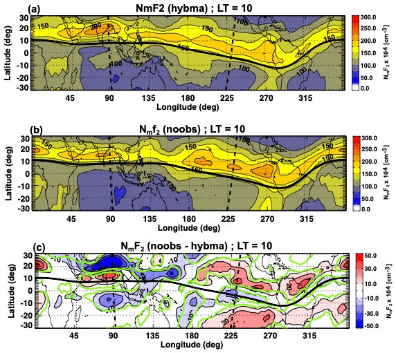
Figure 1NmF2 in units of 104 cm−3 for all locations at 10:00 LT averaged for 1–10 January 2013: (a) hybma, (b) noobs, and (c) noobs minus hybma. The oblique dashed black lines highlight the position of SAMI3 slices whose longitudes at the geographic equator are ∼230 and ∼90° and are discussed in text. The magnetic equator is illustrated by a solid black line across longitude. Green contours in (c) identify the locations where the anomalies are statistically significant at least at 95 % confidence level using a t test.
Focusing on the region over the Pacific Ocean near 225° E, this region shows statistically significant differences between the noobs and hybma runs: a decrease in NmF2 at the magnetic equator is flanked by increases in the NmF2 at latitudes corresponding to the peak of the EIA. The symmetry of this structure about the magnetic equator implies a change to the “fountain effect” (e.g., Hanson and Moffett, 1966): the EIA is maintained through E×B drifts that lift ions to higher altitudes that are created at or near the magnetic equator at lower altitudes. Once the vertical E×B drifts lift the plasma to magnetic field lines with higher apex altitudes, the change in the plasma pressure gradient along these longer field lines will cause the ions to diffuse downwards along the magnetic field lines to lower altitudes and higher latitudes. To verify that a stronger fountain effect is taking place at this location, Fig. 2 shows the electron density on nearby SAMI3 slice (longitude at the geographic equator ∼230°) that cuts through the region of the largest differences (see oblique dashed line in Fig. 1). The electron density in hybma (Fig. 2a) shows the typical arced behavior, with isopleths elevated near the magnetic equator with respect to the adjacent latitudes. The largest electron density is found just below 300 km northward of the geographic equator, with a peak value in excess of 180×104 cm−3. This is consistent with the presence of both an active fountain effect and a northward field-aligned neutral wind. The difference plot (Fig. 2b) shows reduced electron density by about 15–30 × 104 cm−3 at the magnetic equator and increased values in excess of 60×104 cm−3 around 5–10° N. This structure is explained by an increased uplift of ions at the magnetic equator followed by transport along geomagnetic field lines due to the effects of neutral winds and gravity. In both simulations, E×B meridional drifts at the magnetic equator lift ions into the upper F region; in the case of the noobs simulation, a stronger uplift of ions followed by gravity and neutral wind transport results in a removal of charges from the magnetic equator and an accumulation at higher latitudes at this time and location. Note that the accumulation of charges is greater in the Northern Hemisphere, which (at this local time) is likely solely the result of forcing by the neutral wind at the hmF2 along these magnetic field lines (Burrell et al., 2012).
If our interpretation of Fig. 2 is correct, the noobs simulation ought to be showing a more prominent upward drift in the morning hours when compared to hybma. Figure 3 shows the 10 d average (panels a and b, 1–10 January 2013) of the SAMI3 meridional E×B drift at the magnetic equator as a function of longitude and LT. At longitudes around 230° E (which corresponds to the location of SAMI3 slice in Fig. 2) and at 10:00 LT, Fig. 3 shows larger E×B drifts in noobs than in hybma. Since the resulting meridional E×B drift is upward during the day, the electric field must be directed toward the east, resulting in an accumulation of positive (negative) charges at dusk (dawn). Thus, our model results illustrate that the simulation without MA observations (noobs) produces a stronger eastward electric field compared to the simulation with full MA observations, accumulating more charges in the dusk and dawn sectors. The stronger upward E×B drifts lift the F-region plasma to higher altitudes where they then diffuse downwards and polewards along the magnetic field lines. Figure 3 results then confirm that the larger EIA seen in Fig. 1c is due to a stronger fountain effect, which was created by unrealistic influences from the MA in the noobs experiment.
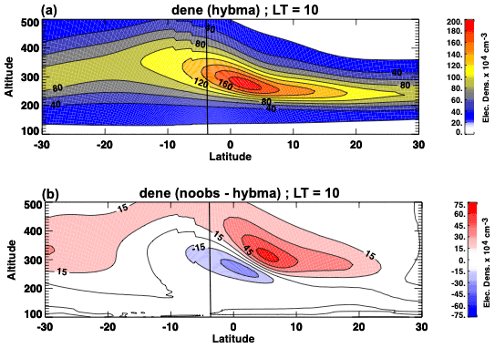
Figure 2Electron density (dene) at 10:00 LT in units of 104 cm−3 along SAMI3 slice whose longitude at the equator is ∼ 230° averaged for the same period as in Fig. 1. The vertical black line identifies the magnetic equator. (a) Electron density in hybma and (b) noobs minus hybma.
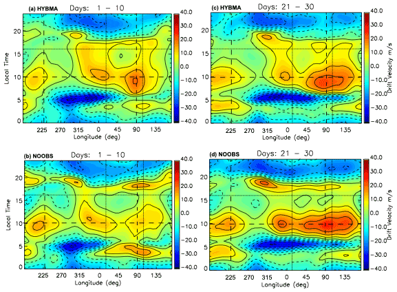
Figure 3The 10 d average of E×B ion drifts in m s−1 obtained from the hybma (a, c) and noobs (b, d) simulations. Panels (a) and (b) are the results of averaging during 1–10 January 2013. Panels (c) and (d) show the drifts averaged during 21–30 January 2013. The dashed black lines identify the approximate longitude (vertical lines) of the morning cases examined for 10:00 LT (horizontal line) and discussed in Fig. 1. The dotted black lines identify the approximate longitude (vertical lines) of the afternoon cases examined for 16:00 LT (horizontal line) and discussed in Figs. 6 and 8.
We now turn to the large differences over the Indian Ocean in Fig. 1. The resulting difference field at this longitude (Fig. 1c) shows an increase in NmF2 just north of the magnetic equator flanked by negative anomalies in both hemispheres. Overall, there is a hemispheric asymmetry, with the largest differences clearly in the Northern Hemisphere. This difference pattern is the opposite of the one shown at the longitude over the Pacific Ocean. There are two mechanisms that may explain these differences: a difference of the meridional E×B drifts resulting in a decrease of the drifts in noobs and a change to the neutral wind-driven ion transport at the F peak. Referring to Fig. 3a and b, we notice that at this longitude (∼90°) the meridional E×B in the noobs simulation is smaller than in hybma. Figure 4 shows the electron density on the SAMI3 slice over the Indian Ocean in hybma (Fig. 4a) and the differences noobs minus hybma (Fig. 4b). The electron density in the reference simulation (hybma) shows the typical arced structure with elevated isopleth of density at the magnetic equator and lowered isopleths in the subtropics: they result from the competing uplift of ions by the meridional E×B drifts at the magnetic equator and gravity. The difference of electron density between noobs and hybma just north of the magnetic equator agrees with the NmF2 differences in Fig. 1. In this case, a weakening of the fountain effect via E×B drifts at this longitude (Fig. 3a, b) creates the pattern in Figs. 1c and 4: both the positive and negative anomalies are necessary to explain the effect of the weakening of the E×B drift. However, this does not explain the substantial asymmetry of the changes across the magnetic equator in Fig. 1c. Thus, we now look at the role of the neutral wind. The field line transport at 300 km (near the F2 peak) in this longitudinal sector (Fig. 5a, b) is northward in both simulations, resulting in ions moved northward across the magnetic equator towards the northern EIA. The difference field noobs minus hybma in Fig. 5c show a large positive (northward) difference in noobs just west of the longitude of the SAMI3 slice in Fig. 4. This pattern of neutral winds illustrates that field-aligned transport in the noobs simulation is stronger than in hybma: the neutral winds around 300 km in noobs move ions across the magnetic equator and accumulate more ions just north of the magnetic equator, setting up the north–south asymmetry in the EIA difference field that is shown in Fig. 1c around 90° E.
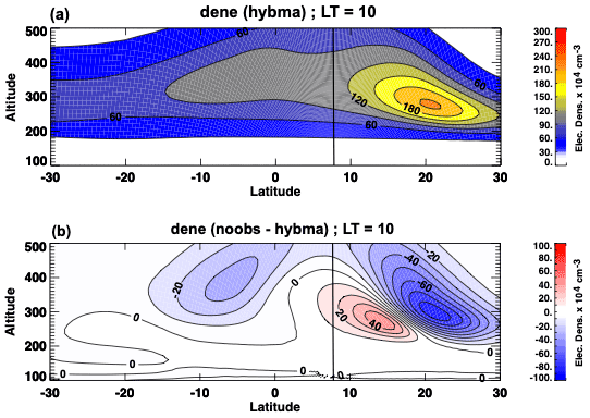
Figure 4Electron density (dene) at 10:00 LT in units of 104 cm−3 along a SAMI3 slice with a longitude of ∼90° E at the geographic equator. Electron density is averaged for the same period as in Fig. 1. The vertical black line identifies the magnetic equator. (a) Electron density in hybma and (b) noobs minus hybma.
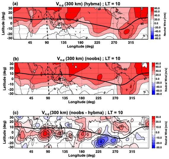
Figure 5Neutral wind Vn,q parallel to geomagnetic field lines at 300 km and 10:00 LT. Units are m s−1. Vn,q is averaged during 1–10 January 2013. The solid black line indicates the location of the magnetic equator, and the dashed line is the location of the SAMI3 slice crossing over the Indian Ocean. (a) Vn,q for hybma, (b) Vn,q for noobs, and (c) Vn,q noobs minus hybma.
3.2 Case 2: 16:00 LT – dynamically active
We now turn our attention to the afternoon hours, with Fig. 6 showing the NmF2 at 16:00 LT. This case illustrates another instance where the noobs and hybma simulations differ. At this LT, the NmF2 peaks broadly between 315 and 90° E longitude in the Northern Hemisphere. The NmF2 in excess of 250×104 cm−3 is broader and more prominent in hybma (Fig. 6a), and the minimum of NmF2 at the magnetic equator extends over more longitudes and is deeper in hybma than in noobs (Fig. 6b).
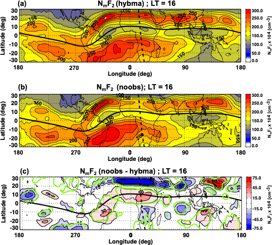
Figure 6NmF2 in units of 104 cm−3 for all locations at 16:00 LT averaged for 1–10 January 2013: (a) hybma, (b) noobs, and (c) noobs minus hybma. The oblique dashed black line highlights the position of SAMI3 slice which crosses the geographic Equator at longitude ∼ 15°). The magnetic equator is described by a solid black line across longitude. Green contours in (c) identify the locations where the differences are statistically significant at least at 95 % level using a t test. Notice that compared to Fig. 1, longitudes have been rotated to have 0° E at the center.
Referring again to Fig. 3a and b, we notice that in the mid-afternoon (16:00 LT) around 15° E longitude the meridional E×B drift is stronger in hybma when compared to noobs. Therefore, in the simulation with MA observations, the electric field is more eastward (i.e., positive) when MA observations are used, resulting in stronger uplift of ions toward the F peak. Figure 7 shows the magnetic field-aligned component of the neutral wind at 300 km as a function of location at 16:00 LT. Note that the noobs run has a stronger northward component along the SAMI3 slice crossing over Africa (∼16°) north of the magnetic equator and a weaker northward component to the south of the magnetic equator. Thus, the noobs run has a larger neutral wind magnitude pushing the plasma northward along the field lines and a weaker fountain effect counteracting the interhemispheric transport. The difference in field parallel transport around the African continent SAMI3 slice, coupled with the different strength of the fountain circulation, explains the hemispheric asymmetry seen in the NmF2 at these longitudes between the two simulations.
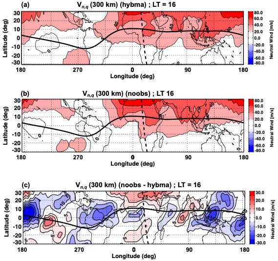
Figure 7Neutral wind Vn,q parallel to geomagnetic field lines at 300 km and 16:00 LT. Units are m s−1. Vn,q is averaged during 1–10 January 2013. The solid black line indicates the location of the magnetic equator, and the dashed line is the location of the SAMI3 slice crossing the geographic equator around longitude ∼16°. (a) Vn,q for hybma, (b) Vn,q for noobs, and (c) Vn,q noobs minus hybma.
3.3 Case 3: 16:00 LT – dynamically quiet
The case studies discussed in Sect. 3.1 and 3.2 illustrate the ionospheric response when the atmosphere is dynamically disturbed, such as during a SSW. As discussed in Sect. 1, anomalous ionospheric behavior is to be expected during these times. We demonstrate now that while this behavior is prominent during dynamically active times, the effect of MA observations is also detectable and statistically significant during dynamically quiet times.
Figure 8 is the equivalent of Fig. 6 but averaged during the last 10 d of January (21–30 January 2013). This time period is well after the disturbance of the SSW on 6 January. We chose the mid-afternoon (16:00 LT) because at this time the electron concentration is higher. During the dynamically quiet times of the end of the month, the largest differences between hybma and noobs shift over the Indonesian maritime region (dashed line). As in the case of the dynamically disturbed days shown in Fig. 6, there is a pronounced local minimum of NmF2 south of the magnetic equator in the hybma simulation, which results in a difference field with a positive NmF2 anomaly near the magnetic equator and negative NmF2 anomalies at sub-tropical latitudes. We note that these anomalies are statistically significant. Similar to the dynamically disturbed times earlier in the month, the anomalous NmF2 later in the month is somewhat asymmetric about the magnetic equator, indicating a continued role of the neutral wind in transporting ions across the magnetic equator (though to a lesser degree). Overall, Fig. 8 shows that the differences in NmF2 between the hybma and noobs simulations are not due to the characteristics of neutral dynamics during a SSW but rather due to the lack of MA observations in the noobs simulation, which plays a role during all types of background conditions.
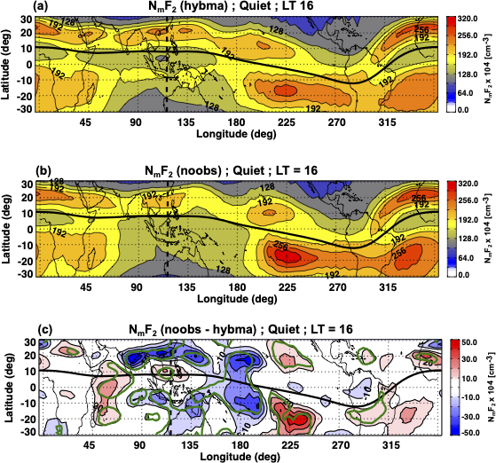
Figure 8As in Fig. 6, NmF2 in units of 104 cm−3 for all locations at 16:00 LT averaged for 21–30 January 2013: (a) hybma, (b) noobs, and (c) noobs minus hybma. The dashed black line highlights the position of SAMI3 slice crossing the geographic equator over the Indian Ocean at a longitude of ∼ 117°. The magnetic equator is described by a solid black line across longitude. Green contours in (c) identify the locations where the differences are statistically significant at least at the 95 % level using a t test.
This study uses two model experiments that couple a thermosphere climate model (WACCM-X), nudged with atmospheric specifications (NAVGEM-HA), to an ionospheric model (SAMI3). The two experiments differ only in the observations that were used to generate the atmospheric specifications: the hybma experiment includes all observations up to the UMLT, and the noobs experiment does not use MA observations above about 40 km. The goal of this study is to demonstrate that a potential future loss of MA observations will have significant negative consequences for our ability to predict the intra-day variability of the neutral atmosphere and ionosphere and is not only impactful for research on the neutral dynamics of the lower thermosphere (as demonstrated by Sassi et al., 2020). The results focused on the NmF2 at a fixed LT, as the peak electron density at the F peak is a well-understood and appropriate diagnostic for ionospheric behavior. Using the NmF2 at fixed LT also allows for an easier interpretation of the differences in terms of differences of non-migrating solar tides, as discussed by Forbes et al. (2006).
The results show that the difference of NmF2 between the two simulations is statistically significant (better than 95 % confidence level) at the selected locations and LT. In the morning (10:00 LT, Sect. 3.1), the largest differences between the two model runs is seen over the Pacific and Indian oceans: a reduction of electric density in noobs near the magnetic equator is accompanied by an increase at adjacent latitudes in the Pacific Ocean, while the opposite signature is seen in the Indian Ocean region. The difference in behavior of NmF2 is found to be caused by a variation in the fountain effect when the MA measurements are not incorporated: stronger (weaker) uplift of ions over the Pacific (Indian) Ocean when MA observations are removed. At different solar local times and geographic locations, in both simulations, the neutral winds introduce a hemispheric asymmetry to the equatorial plasma distribution.
During the afternoon (16:00 LT, Sect. 3.2), the changes in NmF2 over the African continent are similar to those seen in the morning over the Indian Ocean. Examination of the changes along a magnetic meridian shows in fact that the afternoon anomalies are due to the decrease in the magnitude of the meridional E×B drift in noobs when the MA observations are not considered. The magnetic field-aligned component of the neutral wind at 300 km (an altitude chosen as it is just below the peak hmF2) shows that the longitudinal structure of the lower thermospheric neutral wind has also been affected by the differences in MA forcing. This, in turn, changes the magnitude of the interhemispheric transport at this local time, affecting the longitudinal structure of the NmF2.
The first two cases illustrated (Sect. 3.1 and 3.2) include the occurrence of a SSW in the stratosphere, which is known to produce anomalous behavior in the thermosphere and ionosphere; we therefore also examined a dynamically quiet case towards the end of January 2013 (Sect. 3.3). Overall, the effect of removing MA observations from the atmospheric specifications during a dynamically quiet period is consistent with the more dynamically disturbed cases, although showing a more muted response. This indicates that a dynamically disturbed atmosphere is not required for MA observations to impact predictions of ionospheric structure, although a disturbed state can mediate the magnitude of the impact.
The zonally articulated response in NmF2 in all cases due to the exclusion of MA observations indicates that there are differences in the amplitude of non-migrating solar tides. The zonal structure of the difference field indicates prominent wave-3 or wave-4 modes at fixed LT, which is consistent with past findings. For instance, Sassi et al. (2020) showed that the simulation without MA observations (i.e., noobs) produces much larger non-migrating tides, DE3 and DE2. These solar tides are expected to be visible in NmF2 as wave-4 and wave-3 patterns, which are known to impact the structure of the F-region ionosphere (Immel et al., 2006) when plotted at fixed LT.
Finally, we compare the results of these runs to total electron content (TEC) observations made at a nearby longitude slice just eastward of the one shown in Fig. 6 at 110° apex longitude. This longitude slice lies over portions of Africa and Europe that are sufficiently instrumented to provide coverage of the lower latitude region that includes the EIA. For each day of the model simulations, vertical TEC (VTEC) was selected within 3° (for the model runs) or within 5° (for the observational data) and between 15:45 and 16:15 LT. Then, the mean VTEC was calculated at a 1° latitude resolution. Figure 9b shows the geographic longitude of the observations and nearby model data used in our analysis. Figure 9a shows the result of this averaging process, with the noobs run marked by navy circles, the hybma run marked by light blue squares, and the observed VTEC from MIT Haystack (Rideout and Coster, 2006) marked by slate blue triangles.
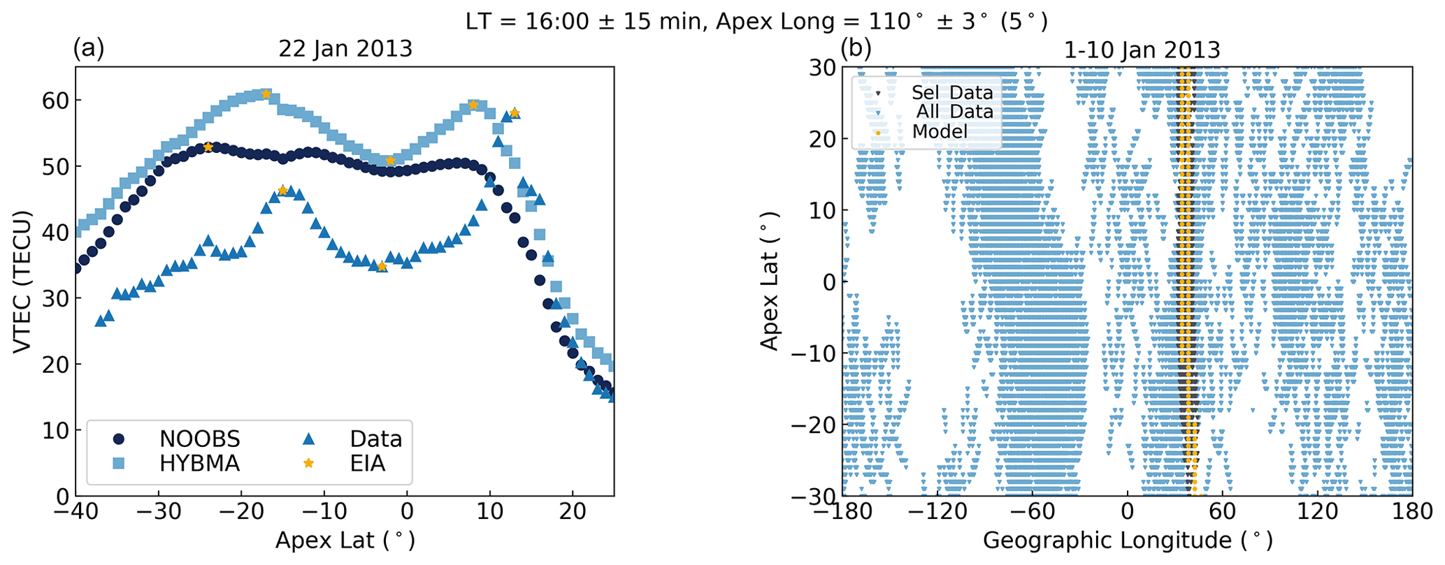
Figure 9(a) Mean VTEC as a function of Apex magnetic latitude at 16:00 LT at 110° magnetic apex longitude on 22 January 2013. The noobs results are marked by navy circles, the hybma results are marked by light-blue squares, and the observation data are marked by slate-blue triangles. The EIA peak and trough locations (or only a central peak, as is the case in the noobs results) are marked by orange stars. (b) Geographic longitude and magnetic latitudes of all available data (light-blue circles) and the selected data (dark-blue circles) used to assemble the statistics of Tables 1 and 2; the corresponding model data (orange circle) are also shown. The panel was constructed for 1–10 January 2013 and is provided here for reference to show that observational data are broadly located at ∼36° E.
Figure 9 shows a day where the two model runs have differing low-latitude VTEC distributions, with neither of them fully agreeing with the observed data. The first level of disagreement is the bias between the model and observations. Depending on the neutral atmospheric composition and density, the SAMI3 model tends to overestimate the ionospheric plasma density. When MSIS is used to provide the background density, as is the case in Fig. 9, this difference is on the order of ∼ 10 TECU near the equator. These differences are most obvious in the VTEC, as it is vertically integrated and exacerbates the problem. Figure 9 also shows the three potential configurations of the low-latitude VTEC encountered during this study: no dual-EIA peak (No; shown by the noobs data), a higher northern EIA peak (North; shown by the observational data), and a higher southern EIA peak (South; shown by the hybma data). We will compare the state of the EIA between the observations and the model runs by determining the times when the modeled and observed EIA had the same configuration.
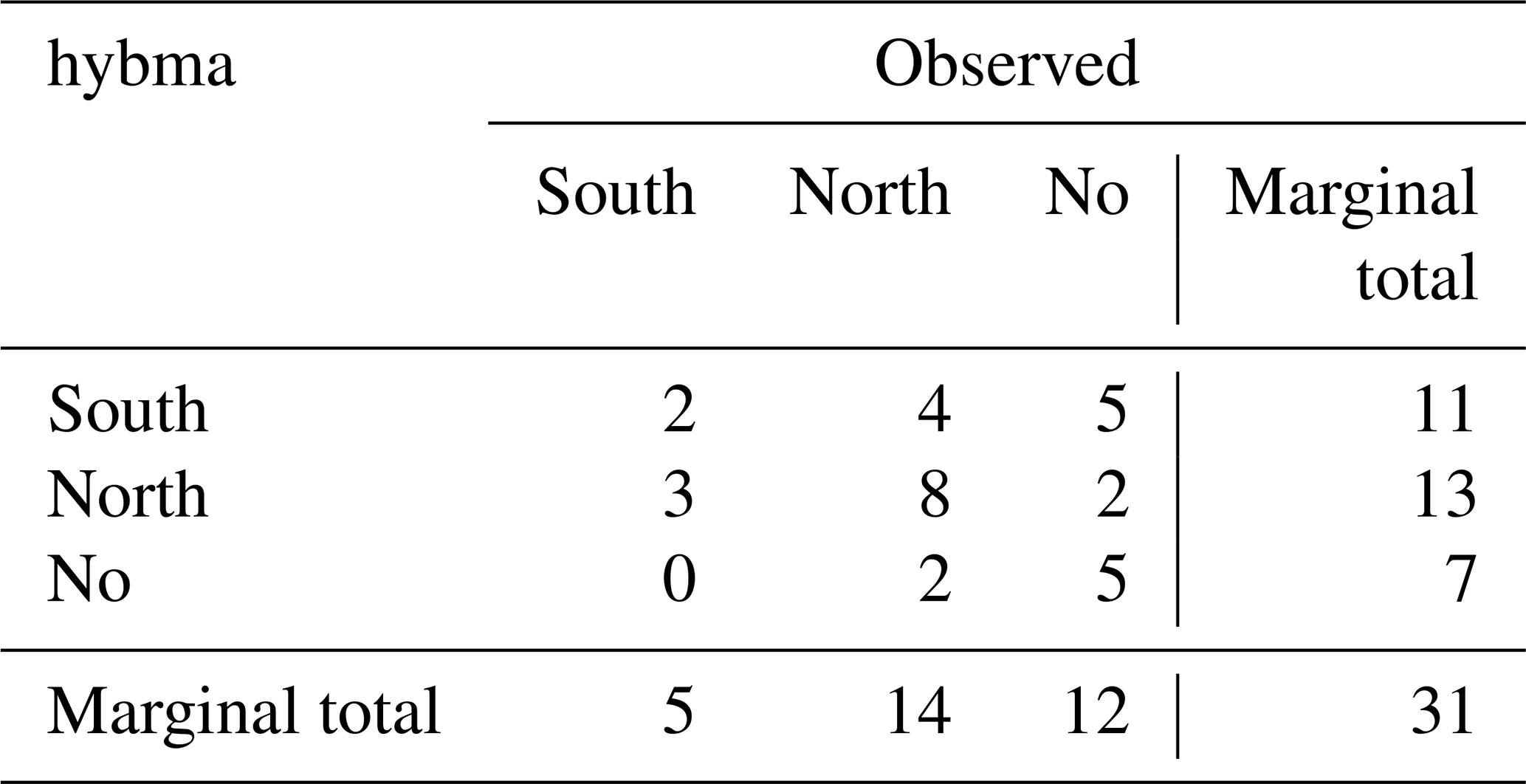
Tables 1 and 2 show the number of days in the month of January 2013 where each model run had a particular EIA configuration and how this compares to the observed EIA configuration. Comparing the two tables shows that introducing MA observations in the hybma run improves the agreement between the observations and the model. This occurs specifically with an increase of the number of days; both the model and observations show an EIA with a dominant northern peak: noobs had 6 d in this EIA configuration, three of which agreed with the observations, and hybma had 13 d in this EIA configuration, 8 of which agreed with the observations. As this is the dominant state in the observations (14 d in total), it greatly improves the overall agreement. This area of change confirms that the improved lower atmospheric boundary does a better job specifying the upper thermospheric wind, which drives the EIA hemispheric asymmetries.
Table 1EIA configuration agreement between noobs and observed VTEC at 110° magnetic apex longitude, 16:00 LT.
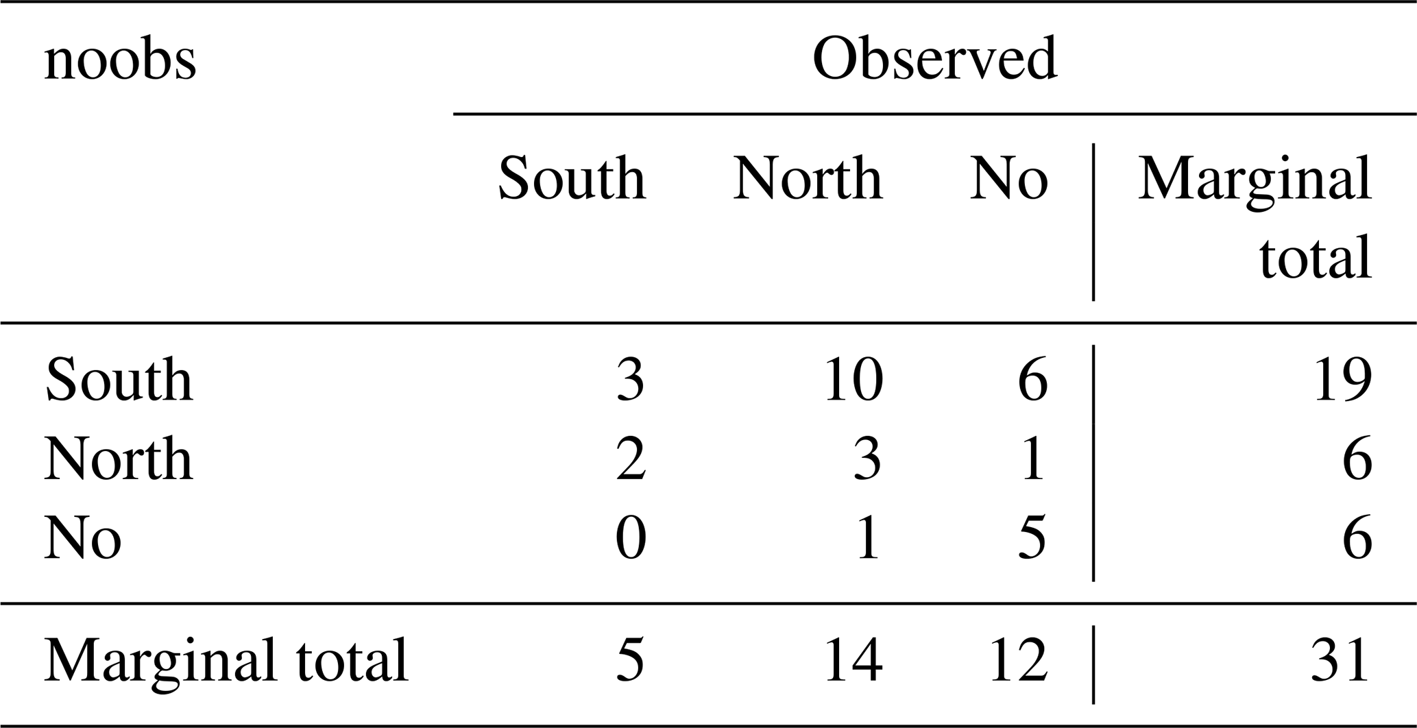
Table 2EIA configuration agreement between hybma and observed VTEC at 110° magnetic apex longitude, 16:00 LT.
The results of this study support the thesis presented in the Introduction: the absence of MA (above 40 km) observations has important and statistically significant consequences for our ability to predict the structure and variability of the ionosphere and upper atmosphere. The impact of the MA observations on the E-region conductivity (which drives the meridional E×B drift) and the thermospheric neutral winds demonstrate that this region is an essential piece that must be understood to fully grapple with interactions between the neutral atmosphere and the ionosphere. At lower latitudes, multiple types of interactions between the thermosphere and ionosphere can lead to ion transport that affects the F-region peak density distribution. Model runs driven with incomplete MA observations may have anomalous neutral wind at E-region altitudes, which leads to an aberrant fountain effect through electrodynamic interactions. They may also have atypical F-region neutral winds that cause abnormal hemispheric electron density distributions, such as a higher electron density in one hemisphere or a decrease in the seasonal EIA asymmetries.
Strictly speaking, these results apply only to the modeling system we have examined. Other modeling systems (for example, systems that assimilate ionospheric data) may see different impacts on the ionospheric state. It is possible that assimilating sufficient data from appropriate ionospheric and thermospheric datasets could mitigate the need for MA observations for ionospheric predictions. To the best of our knowledge, this is the first study that attempts to investigate how a future lack of observations in the MA potentially impacts the upper atmosphere and ionosphere. Given the importance for civilian and military applications of high-fidelity predictions in the upper atmosphere and ionosphere, it is necessary to continue and expand these studies, including examining results from other modeling systems.
SD-WACCM-X (https://www.cesm.ucar.edu/models/cesm2/download, Liu et al., 2018) simulation output and NAVGEM-HA (https://map.nrl.navy.mil, McCormack et al., 2017; Eckermann et al., 2018) atmospheric specifications are archived at the Naval Research Laboratory. The source code and forcing datasets of the SD-WACCM-X are available from the NCAR website at http://www.cesm.ucar.edu/ (last access: 1 April 2022). GPS TEC used in this study is publicly available from the Madrigal database (https://w3id.org/cedar?experiment_list=experiments3/2013/gps/XXjan13&file_list=los_201301XX.001.h5, Coster, 2013) and was converted into magnetic coordinates using apexpy (van der Meeren et al., 2023, https://doi.org/10.5281/zenodo.7818719).
FS conceptualized this study and its methodology, led the writing, and performed the model analysis. AGB led the physical analysis and contributed to both the writing and model analysis. SEM contributed to the physical and model analysis, as well as editing. JLT performed model runs and contributed to the writing. JPM contributed to the writing and model analysis.
The contact author has declared that none of the authors has any competing interests.
Publisher's note: Copernicus Publications remains neutral with regard to jurisdictional claims made in the text, published maps, institutional affiliations, or any other geographical representation in this paper. While Copernicus Publications makes every effort to include appropriate place names, the final responsibility lies with the authors.
Fabrizio Sassi, Angeline G. Burrell, and Sarah E. McDonald acknowledge the support of the Office of Naval Research. This work is supported in part by a grant of computer time from the DOD High Performance Computing Modernization Program at the US Navy DOD Supercomputing Resource Center (NAVO).
GPS TEC data products and access through the Madrigal distributed data system are provided to the community by the Massachusetts Institute of Technology under support from U.S. National Science Foundation grant AGS-1242204. Data for the TEC processing are provided by the following organizations: UNAVCO; Scripps Orbit and Permanent Array Center; Institut Geographique National, France; International GNSS Service; the Crustal Dynamics Data Information System (CDDIS); the National Geodetic Survey; Instituto Brasileiro de Geografia e Estatística; RAMSAC CORS of Instituto Geográfico Nacional de la República Argentina; Arecibo Observatory; Low-Latitude Ionospheric Sensor Network (LISN); Topcon Positioning Systems, Inc.; Canadian High Arctic Ionospheric Network; Institute of Geology and Geophysics, Chinese Academy of Sciences; the China Meteorology Administration; Centro di Niveau des Eaux Littorales Ricerche Sismogiche; Système d'Observation du (SONEL), RENAG, REseau NAtional GPS permanent; and GeoNet – the official source of geological hazard information for New Zealand.
This research has been supported by the Office of Naval Research (6.1 funding).
This paper was edited by Vivien Wendt and reviewed by two anonymous referees.
Alken, P., Thébault, E., Beggan, C. D., Amit, H., Aubert, J., Baerenzung, J., Bondar, T. N., Brown, W. J., Califf, S., Chambodut, A., Chulliat, A., Cox, G. A., Finlay, C. C., Fournier, A., Gillet, N., Grayver, A., Hammer, M. D., Holschneider, M., Huder, L., Hulot, G., Jager, T., Kloss, C., Korte, M., Kuang, W., Kuvshinov, A., Langlais, B., Léger, J. M., Lesur, V., Livermore, P. W., Lowes, F. J., Macmillan, S., Magnes, W., Mandea, M., Marsal, S., Matzka, J., Metman, M. C., Minami, T., Morschhauser, A., Mound, J. E., Nair, M., Nakano, S., Olsen, N., Pavón-Carrasco, F. J., Petrov, V. G., Ropp, G., Rother, M., Sabaka, T. J., Sanchez, S., Saturnino, D., Schnepf, N. R., Shen, X., Stolle, C., Tangborn, A., Tøffner-Clausen, L., Toh, H., Torta, J. M., Varner, J., Vervelidou, F., Vigneron, P., Wardinski, I., Wicht, J., Woods, A., Yang, Y., Zeren, Z., and Zhou, B.: International Geomagnetic Reference Field: the thirteenth generation, Earth Planets Space, 73, 49, https://doi.org/10.1186/s40623-020-01288-x, 2021. a
Burrell, A. and Heelis, R.: The influence of hemispheric asymmetries on field-aligned ion drifts at the geomagnetic equator, Geophys. Res. Lett., 39, L19101, https://doi.org/10.1029/2012GL053637, 2012. a
Burrell, A., Heelis, R., and Stoneback, R.: Equatorial longitude and local time variations of topside magnetic field-aligned ion drifts at solar minimum, J. Geophys. Res., 117, A04304, https://doi.org/10.1029/2011JA017264, 2012. a
Coster, A.: MIT/Haystack Observatory, Data from the CEDAR Madrigal database [data set], XX in the URL is the day of month, https://w3id.org/cedar?experiment_list=experiments3/2013/gps/XXjan13&file_list=los_201301XX.001.h5 (last access: 3 October 2023), 2013. a
Eckermann, S. D., Hoppel, K. W., Coy, L., McCormack, J. P., Siskind, D., Nielsen, K., Kochenash, A., Stevens, M. H., Englert, C. R., Singer, W., and Hervig, M.: High-Altitude data assimilation system experiments for the northern summer mesosphere season of 2007, J. Atmos. Sol.-Terr. Phy., 71, 531–551, https://doi.org/10.1016/j.jastp.2008.09.036, 2009. a
Eckermann, S. D., Ma, J., Hoppel, K. W., Kuhl, D., Allen, D. R., Doyle, J., Viner, K. C., Ruston, B. C., Baker, N. L., Swadley, S. D., Whitcomb, T. R., Reynolds, C. A., Xu, L., Kaifler, N., Keifler, B., Reid, I. M., Murphy, D. J., and Love, P. T.: High-Altitude (0–100 km) global atmospheric reanalysis system: Description and application to the 2014 austral winter of the Deep Propagating Gravity Wave Experiment (DEEPWAVE), Mon. Weather Rev., 146, 2639–2666, https://doi.org/10.1175/MWR-D-17-0386.1, 2018 (data available at: https://map.nrl.navy.mil (cd to map/pub/nrl/navgem-ha/2013) in netCDF format, last access: 1 April 2022). a, b, c
Emmert, J. T., Drob, D. P., Picone, J. M., Siskind, D. E., Jones Jr., M., Mlynczak, M. G., Bernath, P. F., Chu, X., Doornbos, E., Funke, B., Goncharenko, L. P., Hervig, M. E., Schwartz, M. J., Sheese, P. E., Vargas, F., Williams, B. P., and Yuan, T.: NRLMSIS 2.0: A Whole-Atmosphere Empirical Model of Temperature and Neutral Species Densities, Earth Space Sci., 8, e2020EA001321, https://doi.org/10.1029/2020EA001321, 2021. a
Erwin, S. and Berger, B.: A race against time to replace aging military weather satellites, https://spacenews.com/a-race-against-time-to-replace-aging-military-weather-satellites/ (last access: 17 December 2023), 2021. a
Fang, T., Akmaev, R., Fuller-Rowell, T., Wu, F. Maruyama, N., and Millward, G.: Longitudinal and day-to-day variability in the ionosphere from lower atmosphere tidal forcing, Geophys. Res. Lett., 40, 2523–2528, https://doi.org/10.1002/grl.50550, 2013. a
Forbes, J. and Zhang, X.: Quasi 2-day oscillation of the ionosphere: A statistical study, J. Atmos. Sol.-Terr. Phy., 59, 1025–1034, https://doi.org/10.1016/S1364-6826(96)00175-7, 1997. a
Forbes, J., Palo, S., and Zhang, X.: Variability of the ionosphere, J. Atmos. Sol.-Terr. Phy., 62, 685–693, https://doi.org/10.1016/S1364-6826(00)00029-8, 2000. a
Forbes, J., Russell, J., Miyahara, S., Zhang, X., Palo, S., Mlynczak, M., Mertens, C., and Hagan, M.: Troposphere-thermosphere tidal coupling as measured by the SABER instrument on TIMED during July–September 2002, J. Geophys. Res., 111, A10S06, https://doi.org/10.1029/2005JA011492, 2006. a, b
Forbes, J., Zhang, X., Palo, S., Russell, J., Mertens, C., and Mlynczak, M.: Tidal variability in the ionospheric dynamo region, J. Geophys. Res., 113, A02310, https://doi.org/10.1029/2007JA012737, 2008. a
Fuller‐Rowell, T., Fang, T., Wang, H., Matthias, V., Hoffmann, P., Hocke, K., and Studer, S.: Impact of Migrating Tides on Electrodynamics During the January 2009 Sudden Stratospheric Warming, in: Ionospheric space weather: longitude and hemispheric dependencies and lower atmosphere forcing, edited by: Fuller-Rowell, T., Yizengaw, E., Doherty, P., and Basu, S., Vol. 220 of Geophysical Monograph Series, 165–174, American Geophysical Union, https://doi.org/10.1002/9781118929216.ch14, 2017. a
Goncharenko, L., Coster, A., Chau, L., and Valladares, C.: Impact of sudden stratospheric warmings on equatorial ionization anomaly, J. Geophys. Res., 115, A00G07, https://doi.org/10.1029/2010JA015400, 2010. a
Hagan, M., Maute, A., Roble, R., Richmond, A., Immel, T., and England, S.: Connections between deep tropical clouds and the Earth's ionosphere, Geophys. Res. Lett., 34, L20109, https://doi.org/10.1029/2007GL030142, 2007. a
Hanson, W. and Moffett, R.: Ionization transport effects in the equatorial F region, J. Geophys. Res., 71, 5559–5572, https://doi.org/10.1029/JZ071i023p05559, 1966. a
Heelis, R.: Electrodynamics in the low and middle latitude ionosphere: a tutorial, J. Atmos. Sol.-Terr. Phy., 66, 825–838, https://doi.org/10.1016/j.jastp.2004.01.034, 2004. a
Hines, C.: Internal atmospheric gravity waves at ionospheric heights, Can. J. Phys., 38, 1441–1481, https://doi.org/10.1139/p60-150, 1960. a
Hoppel, K. W., Eckermann, S. D., Coy, L., Nedoluha, G., and Allen, D. R.: Evaluation of SSMIS upper atmosphere sounding channels for high-altitude data assimilation, Mon. Weather Rev., 141, 3314–3330, https://doi.org/10.1175/MWR-D-13-00003.1, 2013. a
Huba, J., Joyce, G., and Fedder, J.: Sami2 is Another Model of the Ionosphere (SAMI2): A new low-latitude ionosphere model, J. Geophys. Res., 105, 23035–23053, https://doi.org/10.1029/2000JA000035, 2000. a
Huba, J., Joyce, G., Krall, J., Siefring, C., and Bernhardt, P.: Self-consistent modeling of equatorial dawn density depletions, Geophys. Res. Lett., 37, L03104, https://doi.org/10.1029/2009GL041492, 2010. a
Immel, T., E., S., England, S., Henderson, S., Hagan, M., Mende, S., Frey, H., Swenson, C., and Paxton, L.: Control of equatorial ionospheric morphology by atmospheric tides, Geophys. Res. Lett., 33, L15108, https://doi.org/10.1029/2006GL026161, 2006. a, b
Jin, H., Miyoshi, Y., Pancheva, D., Mukhtarov, P., Fujiwara, H. J., and Shinagawa, H.: Response of migrating tides to the stratospheric sudden warming in 2009 and their effects on the ionosphere studied by a whole atmosphere-ionosphere model GAIA with COSMIC and TIMED/SABER observations, J. Geophys. Res., 117, A10323, https://doi.org/10.1029/2012JA017650, 2012. a
Kuhl, D., Rosmond, T., Bishop, C., McLay, J., and Baker, N.: Comparison of hybrid ensemble/4DVAR and 4DVAR within the NAVDAS-AR data assimilation framework, Mon. Weather Rev., 141, 2740–2758, https://doi.org/10.1175/MWR-D-12-00182.1, 2013. a
Laprise, R.: The resolution of spectral models, B. Am. Meteorol. Soc., 73, 1453–1455, 1992. a
Laundal, K. M. and Richmond, A. D.: Magnetic Coordinate Systems, 206, 27–59, https://doi.org/10.1007/s11214-016-0275-y, 2017. a
Liu, H.-L.: Variability and predictability of the space environment as related to lower atmosphere forcing, Space Weather, 14, 634–658, https://doi.org/10.1002/2016SW001450, 2016. a, b
Liu, H.-L., Sassi, F., and Garcia, R.: Error growth in a whole atmosphere climate model, J. Atmos. Sci., 66, 173–186, https://doi.org/10.1175/2008JAS2825.1, 2009. a
Liu, H.-L., Foster, B., Hagan, M., McInerney, J., Maute, A., Qian, L., Richmond, A., Roble, R., Solomon, S., Garcia, R., Kinnison, D., Marsh, D., Smith, A., Richter, J., Sassi, F., and Oberheide, J.: Thermosphere extension of the Whole Atmosphere Community Climate Model, J. Geophys. Res., 115, A12302, https://doi.org/10.1029/2010JA015586, 2010. a, b
Liu, H.-L., Yudin, V., and Roble, R.: Day‐to‐day ionospheric variability due to lower atmosphere perturbations, Geophys. Res. Lett., 40, 665–670, https://doi.org/10.1002/grl.50125, 2013. a
Liu, H.-L., Bareedn, C., Foster, B., Lauritzen, P., Liu, J., Lu, G., Marsh, D., Maute, A., McInerney, J., Pedatella, N., Qian, L., Richmond, A., Roble, R., Solomon, S., Vitt, F., and Wang, W.: Development and validation of the Whole Atmosphere Community Climate Model with thermosphere and ionosphere extension (WACCM-X 2.0), J. Adv. Model. Earth Sy., 10, 381–402, https://doi.org/10.1002/2017MS001232, 2018 (data available at: https://www.cesm.ucar.edu/models/cesm2/download, last access: 1 April 2022). a, b
McCormack, J., Hoppel, K., Kuhl, D., de Wit, R., Stober, G., Espy, P., Baker, N., Brown, P., Fritts, D., Jacobi, C., Janches, D., Mitchell, N., Ruston, B., Swadley, S., Viner, K., Whitcomb, T., and Hibbins, R.: Comparison of mesospheric winds from high-altitude meteorological analysis system and meteor radar observations during the boreal winters of 2009–2010 and 2012–2013, J. Atmos. Sol.-Terr. Phy., 154, 132–166, https://doi.org/10.1016/j.jastp.2016.12.007, 2017 (data available at: https://map.nrl.navy.mil (cd to map/pub/nrl/navgem-ha/2013) in netCDF format, last access: 1 April 2022). a, b, c
McDonald, S., Sassi, F., and Mannucci, A.: SAMI3/SD-WACCM-X simulations of ionospheric variability during northern winter 2009, Space Weather, 13, 568–584, https://doi.org/10.1002/2015SW001223, 2015. a, b
McDonald, S., Sassi, F., Tate, J., McCormack, J., Kuhl, D., Drob, D., Metzler, C., and Mannucci, A.: Impact of non-migrating tides on the low latitude ionosphere during a sudden stratospheric warming event in January 2010, J. Atmos. Sol.-Terr. Phy., 171, 188–200, https://doi.org/10.1016/j.jastp.2017.09.012, 2018. a, b
Millward, G. H., Muller-Wodrag, I. C. F., Aylward, A. D., Fuller-Rowell, T. J., Richmond, A. D., and Moffett, R. J.: An investigation into the influ- ence of tidal forcing on F region equatorial vertical ion drift using a global ionosphere-thermosphere model with coupled electrodynamics, J. Geophys. Res., 106, 24733–24744, https://doi.org/10.1029/2000JA000342, 2001. a
Pedatella, N. and Maute, A.: Impact of semidiurnal tide on the midlatitude thermospheric wind and ionosphere during sudden stratospheric warmings, J. Geophys. Res., 120, 10740–10753, https://doi.org/10.1002/2015JA021986, 2015. a
Pedatella, N., Reader, K., Anderson, J., and Liu, H.-L.: Application of data assimilation in the whole atmosphere community climate model to the study of day-to-day variability in the middle and upper atmosphere, Geophys. Res. Lett., 40, 4469–4474, https://doi.org/10.1002/grl.50884, 2013. a
Pedatella, N., Liu, H.-L., Marsh, D., Reader, K., Anderson, J., Chau, J., Goncharenko, L., and Siddiqui, T.: Analysis and hindcast experiments of the 2009 sudden stratospheric warming in WACCMX+DART, J. Geophys. Res., 123, 3131–3153, https://doi.org/10.1002/2017JA025107, 2018. a
Pedatella, N., Liu, H.-L., Marsh, D., Reader, K., and Anderson, J. L.: Error growth in the mesosphere and lower thermosphere based on hindcast experiments in a whole atmosphere model, Space Weather, 17, 1442–1460, https://doi.org/10.1029/2019SW002221, 2019. a
Richmond, A.: Ionospheric electrodynamics using magnetix APEX coordinates, J. Geomag. Geoelec., 47, 191–212, https://doi.org/10.1002/2017JA025107, 1995. a
Rideout, W. and Coster, A. J.: Automated GPS processing for global total electron content data, GPS Solut., 10, 219–228, https://doi.org/10.1007/s10291-006-0029-5, 2006. a
Rishbeth, H.: Thermospheric winds and the F-rgion: A review, J. Atmos. Sol.-Terr. Phy., 34, 1–47, https://doi.org/10.1016/0021-9169(72)90003-7, 1972. a
Sassi, F., Liu, H.-L., Ma, J., and Garcia, R.: The lower thermosphere during the northern hemisphere winter of 2009: A modeling study using high-altitude data assimilation products in WACCM-X, J. Geophys. Res., 118, 8954–8968, https://doi.org/10.1002/jgrd.50632, 2013. a
Sassi, F., McCormack, J., and McDonald, S.: Whole atmosphere coupling on intraseasonal and interseasonal time scales: a potential source of increased predictive capability, Radio Sci., 54, 913–933, https://doi.org/10.1029/2019RS006847, 2019. a, b
Sassi, F., McCormack, J., Tate, J., Kuhl, D., and Baker, N.: Assessing the impact of middle atmosphere observations on day-to-day variability in lower thermospheric winds using WACCM-X, J. Atmos. Sol.-Terr. Phy., 212, 105486, https://doi.org/10.1016/j.jastp.2020.105486, 2020. a, b, c, d, e, f, g, h, i
Solomon, S. and Qian, L.: Solar extreme-ultraviolet irradiance for general circulation models, J. Geophys. Res., 110, A10306, https://doi.org/10.1029/2005JA011160, 2005. a
van der Meeren, C., Laundal, K. M., Burrell, A. G., Lamarche, L. L., Starr, G., Reimer, A. S., and Morschhauser, A.: aburrell/apexpy: ApexPy Version 2.0.1, Zenodo [code], https://doi.org/10.5281/zenodo.7818719, 2023. a
VanZandt, T. E., Clark, W. L., and Warnock, J. M.: Magnetic Apex Coordinates: A Magnetic Coordinate System for the Ionospheric F2 Layer, J. Geophys. Res., 77, 2406–2411, https://doi.org/10.1029/JA077i013p02406, 1972. a
Wang, H., Fuller-Rowell, T., Akmaev, R., Hu, M., Kliest, D., and Iredell, M.: First simulations with a whole atmosphere data assimilation and forecvast system: The January 2009 major sudden stratospheric warming, J. Geophys. Res., 116, A12321, https://doi.org/10.1029/2011JA017081, 2011. a, b
Weimer, D.: Models of high-latitude electric potentials derived with a least error fit of spherical harmonic coefficients, J. Geophys. Res., 100, 19595–19607, https://doi.org/10.1029/95JA01755, 1995. a
Weimer, D.: Improved ionospheric electrodynamics models and application to calculating Joule heating rates, J. Geophys. Res., 110, A05306, https://doi.org/10.1029/2004JA010884, 2005. a
Wu, T.-Y., Liu, J.-Y., Chang, L., Lin, C.-H., and Chiu, Y.-C.: Equatorial ionization anomaly response to lunar phase and stratospheric sudden warming, Sci. Rep., 11, 14695, https://doi.org/10.1038/s41598-021-94326-x, 2021. a